THE EFFECTS OF LONG-DURATION EARTHQUAKES ON CONCRETE BRIDGES WITH POORLY CONFINED COLUMNS THERON JAMES THOMPSON

Transcription

1 THE EFFECTS OF LONG-DURATION EARTHQUAKES ON CONCRETE BRIDGES WITH POORLY CONFINED COLUMNS By THERON JAMES THOMPSON A thesis submitted in partial fulfillment of the requirement for the degree of MASTERS OF SCIENCE IN CIVIL ENGINEERING WASHINGTON STATE UNIVERSITY Department of Civil and Environmental Engineering DECEMBER 2004

2 To the Faculty of Washington State University: The members of the Committee appointed to examine the thesis of THERON JAMES THOMPSON find it satisfactory and recommend that it be accepted. Chair ii

3 Acknowledgements Funding for this project has been provided by the Federal Highway Administration. Information, earthquake records, and drawings of bridges in Western Washington State were supplied by the Washington State Department of Transportation. Special thanks goes to Dr. Cofer for his invaluable help and guidance throughout this project. I would like to thank Dr. McDaniel and Dr. McLean for their assistance during the project. Special thanks goes to Seth Stapleton for all of the work he did in the laboratory testing. I would especially like to thank my mother and father for their continual support and encouragement. iii

4 THE EFFECTS OF LONG-DURATION EARTHQUAKES ON CONCRETE BRIDGES WITH POORLY CONFINED COLUMNS Abstract By Theron James Thompson, M.S. Washington State University December 2004 Chair: William F. Cofer The main goals of this research were to implement a mathematical damage model for older, poorly confined, concrete bridge columns into the computer program WSU-NEABS and then evaluate bridge response to long-duration earthquakes. Two actual highway bridges were modeled with finite element spine models and analyzed with this modified version of the nonlinear analysis program. The analyses were done in two stages, the first of which included analyzing the bridges subjected to a suite of ten earthquakes. The suite of earthquakes incorporated short and long-duration events. Results from the analyses were used to predict the response of the bridges and determine if long-duration earthquakes significantly change their response. The second stage of the analyses involved a parametric study in which the soil stiffness at the column bases and abutments was varied. In each case, the response of the bridge was then compared to that of the original model in the first stage. The results were also evaluated to determine if long-duration earthquakes were more damaging with these variations. A simplified bent model was also constructed to represent the center pier of iv

5 the bridge with the most critical response. This model was then analyzed to determine if a bent model can accurately model the response of the bridge, or if the entire bridge model is necessary. The results from the analyses show that neither the short or long-duration events will cause major damage in the bridge columns for the bridges considered. However, the analyses do show that the bridges are predicted to have issues with pounding and possible failure of the bearing pads. The second stage of the analyses shows that the current modeling techniques used by the Washington Department of Transportation, in which rollers are applied at the abutments and the column bases are fixed, predicts more damage to the bridge columns compared to results from more refined foundation models. Thus, the present techniques are a conservative practice for the bridge columns. However, models based on these techniques under predict the pounding at the expansion joints and possible failure of the bearing pads, thus representing an unconservative approach these elements in the bridge. v

6 Table of Contents ACKNOWLEDGEMENTS...III ABSTRACT... IV TABLE OF CONTENTS... VI LIST OF TABLES... XIV LIST OF FIGURES... XXI CHAPTER INTRODUCTION Pre-1970 Bridge Column Design Research Objectives Seismicity of Western Washington State Program Modification Bridge Modeling Bridge Analysis... 6 CHAPTER TWO...7 vi

7 LITERATURE REVIEW Introduction Current Damage Analysis Methods Damage Models Based on Strength and Stiffness Degradation Damage Models Based on Measures of Deformation and/or Ductility Damage Models Based on Energy Dissipation Damage Models Based on Hybrid Formulations Damage Models Based on More Complex Fatigue Models Additional Topics CHAPTER WSU-NEABS COMPUTER PROGRAM The History of the Computer Program WSU-NEABS Review of the Previous Beam-Column Element Previous Damage Coefficient Yield Function Modification of WSU-NEABS Modification of the Damage Model Modification of the Hysteresis Model for the Beam-Column Element Examples vii

8 3.4.1 Example Example Example Damage Level Comparison CHAPTER SEISMIC ANALYSIS OF BRIDGES UNDER LONG-DURATION LOADING WSDOT Bridge 5/ Introduction Description of the Bridge Structural Model Seismic Excitation WSDOT Bridge 5/ Introduction Description of the Bridge Structural Model Seismic Excitation CHAPTER ANALYTICAL RESULTS AND INTERPRETATION Introduction viii

9 5.2 Bridge 5/ Modified Peru Earthquake Modified Chile Earthquake Bridge 5/ Modified Peru Earthquake Modified Chile Earthquake Summary of all other Earthquakes Bridge 5/ Bridge 5/ CHAPTER SOIL-STRUCTURE PARAMETRIC STUDY AND BENT MODEL COMPARISON Introduction Soil-Structure Parametric Study Protocol Results and Interpretation Run No Run No Run No Run No Run No ix

10 6.3.6 Run No Run No Run No Run No Run No Run No Run No Run No Bent Model Comparison CHAPTER SUMMARY AND CONCLUSIONS Summary Analyses with Constant Soil Stiffness Analyses with Varying Soil Stiffness Bent Model Comparison Recommendations for Future Work REFERENCES APPENDIX A x

11 ADDITIONAL TIME HISTORIES USED IN STUDY APPENDIX B APPENDIX C ADDITIONAL OUTPUT FROM STUDY C.1 Introduction C.2 Bridge 5/518; Unmodified Peru C.3 Bridge 5/518; Unmodified Chile Earthquake C.4 Bridge 5/518; Mexico City 475-Year Earthquake C.5 Bridge 5/518; Mexico City 950-Year Earthquake C.6 Bridge 5/518; Olympia 475-Year Earthquake C.7 Bridge 5/518; Olympia 950-Year Earthquake C.8 Bridge 5/518; Kobe 475-Year Earthquake C.9 Bridge 5/518; Kobe 950-Year Earthquake C.10 Bridge 5/826; Unmodified Peru Earthquake C.11 Bridge 5/826; Unmodified Chile Earthquake C.12 Bridge 5/826; Mexico City 475-Year Earthquake xi

12 C.13 Bridge 5/826; Mexico City 950-Year Earthquake C.14 Bridge 5/826; Olympia 475-Year Earthquake C.15 Bridge 5/826; Olympia 950-Year Earthquake C.16 Bridge 5/826; Kobe 475-Year Earthquake C.17 Bridge 5/826; Kobe 950-Year Earthquake APPENDIX D ADDITIONAL OUTPUT FROM SOIL-STRUCTURE STUDY D.1 Introduction D.2 Run No D.3 Run No D.4 Run No D.5 Run No D.6 Run No D.7 Run No D.8 Run No D.9 Run No xii

13 D.10 Run No D.11 Run No D.12 Run No D.13 Run No D.14 Run No xiii

14 List of Tables Table Structural Properties of Column Table Summary of Standard Cyclic Protocol (Stapleton 2004) Table Structural Properties of Column Table Structural Properties for Columns, Crossbeams, and Deck Beams Table Yield Function Constants for the Columns Table Stiffness Properties for Soil Springs (k/in) Table Input Parameters for Expansion Joints Table Structural Properties for Columns and Crossbeams Table Yield Function Constants for the Columns Table Stiffness Properties for Soil Springs (k/in) Table Input Parameters for Expansion Joints Table Maximum Moment (kip-in) at the Top and Bottoms of Columns, Table Maximum Shear (kips) in the Columns, Modified Peru Earthquake Table Maximum Shear (kips) at the Abutments, Modified Peru Earthquake 98 Table Maximum Moment (kip-in) at the Top and Bottoms of Columns, Table Maximum Shear (kips) in the Columns, Modified Chile Earthquake. 108 Table Maximum Shear (kips) at the Abutments, Modified Chile Earthquake Table Maximum Moment (kip-in) at the Top and Bottoms of Columns, Table Maximum Shear (kips) in the Columns, Modified Peru Earthquake Table Maximum Shear (kips) at the Abutments, Modified Peru Earthquake xiv

15 Table Maximum Moment (kip-in) at the Top and Bottoms of Columns, Table Maximum Shear (kips) in the Columns, Modified Chile Earthquake. 123 Table Maximum Shear (kips) at the Abutments, Modified Chile Earthquake Table Results from the Unmodified Peru Earthquake Table Results from the Unmodified Chile Earthquake Table Results from the Mexico City 475-Year Earthquake Table Results from the Mexico City 950-Year Earthquake Table Results from the Olympia 475-Year Earthquake Table Results from the Olympia 950-Year Earthquake Table Results from the Kobe 475-Year Earthquake Table Results from the Kobe 950-Year Earthquake Table Results from the Unmodified Peru Earthquake Table Results from the Unmodified Chile Earthquake Table Results from the Mexico City 475-Year Earthquake Table Results from the Mexico City 950-Year Earthquake Table Results from the Olympia 475-Year Earthquake Table Results from the Olympia 950-Year Earthquake Table Results from the Kobe 475-Year Earthquake Table Results from the Kobe 950-Year Earthquake Table Analysis Protocol Table Maximum Moment (kip-in) at the Top and Bottoms of Columns, Table Maximum Shear (kips) in the Columns, Modified Peru Earthquake,. 153 xv

16 Table Results from the Modified Peru Earthquake, Bridge 5/518, Run No Table Results from the Modified Peru Earthquake, Bridge 5/518, Run No Table Results from the Modified Peru Earthquake, Bridge 5/518, Run No Table Results from the Modified Peru Earthquake, Bridge 5/518, Run No Table Results from the Modified Peru Earthquake, Bridge 5/518, Run No Table Results from the Modified Chile Earthquake, Bridge 5/518, Run No Table Results from the Modified Peru Earthquake, Bridge 5/826, Run No Table Results from the Modified Peru Earthquake, Bridge 5/826, Run No Table Results from the Olympia 950-Year EQ, Bridge 5/518, Run No Table Results from the Kobe 950-Year EQ, Bridge 5/518, Run No Table Results from the Olympia 950-Year EQ, Bridge 5/826, Run No Table Results from the Kobe 950-Year EQ, Bridge 5/826, Run No Table Maximum Moment (kip-in) at the Top and Bottoms of Columns Table Maximum Shear (kips) at the Top and Bottoms of Columns Table Summary of Results for Bridge 5/ xvi

17 Table Summary of Results for Bridge 5/ Table Analysis Protocol Table Summary of Results for Bridge 5/ Table Summary of Results for Bridge 5/ Table C.2-1 Maximum Moment (kip-in) at the Top and Bottoms of Columns Table C.2-2 Maximum Shear (kips) in the Columns Table C.2-3 Maximum Shear (kips) at the Abutments Table C.3-1 Maximum Moment (kip-in) at the Top and Bottoms of Columns Table C.3-2 Maximum Shear (kips) in the Columns Table C.3-3 Maximum Shear (kips) at the Abutments Table C.4-1 Maximum Moment (kip-in) at the Top and Bottoms of Columns Table C.4-2 Maximum Shear (kips) in the Columns Table C.4-3 Maximum Shear (kips) at the Abutments Table C.5-1 Maximum Moment (kip-in) at the Top and Bottoms of Columns Table C.5-2 Maximum Shear (kips) in the Columns Table C.5-3 Maximum Shear (kips) at the Abutments Table C.6-1 Maximum Moment (kip-in) at the Top and Bottoms of Columns Table C.6-2 Maximum Shear (kips) in the Columns Table C.6-3 Maximum Shear (kips) at the Abutments Table C.7-1 Maximum Moment (kip-in) at the Top and Bottoms of Columns Table C.7-2 Maximum Shear (kips) in the Columns Table C.7-3 Maximum Shear (kips) at the Abutments Table C.8-1 Maximum Moment (kip-in) at the Top and Bottoms of Columns xvii

18 Table C.8-2 Maximum Shear (kips) in the Columns Table C.8-3 Maximum Shear (kips) at the Abutments Table C.9-1 Maximum Moment (kip-in) at the Top and Bottoms of Columns Table C.9-2 Maximum Shear (kips) in the Columns Table C.9-3 Maximum Shear (kips) at the Abutments Table C.10-1 Maximum Moment (kip-in) at the Top and Bottoms of Columns Table C.10-2 Maximum Shear (kips) in the Columns Table C.10-3 Maximum Shear (kips) at the Abutments Table C.11-1 Maximum Moment (kip-in) at the Top and Bottoms of Columns Table C.11-2 Maximum Shear (kips) in the Columns Table C.11-3 Maximum Shear (kips) at the Abutments Table C.12-1 Maximum Moment (kip-in) at the Top and Bottoms of Columns Table C.12-2 Maximum Shear (kips) in the Columns Table C.12-3 Maximum Shear (kips) at the Abutments Table C.13-1 Maximum Moment (kip-in) at the Top and Bottoms of Columns Table C.13-2 Maximum Shear (kips) in the Columns Table C.13-3 Maximum Shear (kips) at the Abutments Table C.14-1 Maximum Moment (kip-in) at the Top and Bottoms of Columns Table C.14-2 Maximum Shear (kips) in the Columns Table C.14-3 Maximum Shear (kips) at the Abutments Table C.15-1 Maximum Moment (kip-in) at the Top and Bottoms of Columns Table C.15-2 Maximum Shear (kips) in the Columns Table C.15-3 Maximum Shear (kips) at the Abutments xviii

19 Table C.16-1 Maximum Moment (kip-in) at the Top and Bottoms of Columns Table C.16-2 Maximum Shear (kips) in the Columns Table C.16-3 Maximum Shear (kips) at the Abutments Table C.17-1 Maximum Moment (kip-in) at the Top and Bottoms of Columns Table C.17-2 Maximum Shear (kips) in the Columns Table C.17-3 Maximum Shear (kips) at the Abutments Table D.3-1 Maximum Moment (kip-in) at the Top and Bottoms of Columns Table D.3-2 Maximum Shear (kips) in the Columns Table D.4-1 Maximum Moment (kip-in) at the Top and Bottoms of Columns Table D.4-2 Maximum Shear (kips) in the Columns Table D.4-3 Maximum Shear (kips) at the Abutments Table D.5-1 Maximum Moment (kip-in) at the Top and Bottoms of Columns Table D.5-2 Maximum Shear (kips) in the Columns Table D.6-1 Maximum Moment (kip-in) at the Top and Bottoms of Columns Table D.6-2 Maximum Shear (kips) in the Columns Table D.6-3 Maximum Shear (kips) at the Abutments Table D.7-1 Maximum Moment (kip-in) at the Top and Bottoms of Columns Table D.7-2 Maximum Shear (kips) in the Columns Table D.7-3 Maximum Shear (kips) at the Abutments Table D.8-1 Maximum Moment (kip-in) at the Top and Bottoms of Columns Table D.8-2 Maximum Shear (kips) in the Columns Table D.9-1 Maximum Moment (kip-in) at the Top and Bottoms of Columns Table D.9-2 Maximum Shear (kips) in the Columns xix

20 Table D.10-1 Maximum Moment (kip-in) at the Top and Bottoms of Columns Table D.10-2 Maximum Shear (kips) in the Columns Table D.11-1 Maximum Moment (kip-in) at the Top and Bottoms of Columns Table D.11-2 Maximum Shear (kips) in the Columns Table D.12-1 Maximum Moment (kip-in) at the Top and Bottoms of Columns Table D.12-2 Maximum Shear (kips) in the Columns Table D.13-1 Maximum Moment (kip-in) at the Top and Bottoms of Columns Table D.13-2 Maximum Shear (kips) in the Columns Table D.14-1 Maximum Moment (kip-in) at the Top and Bottoms of Columns Table D.14-2 Maximum Shear (kips) in the Columns xx

21 List of Figures Figure The Cascadia Subduction Zone Boundary (NRCan, 2004)... 4 Figure The Cascadia Subduction Zone (NRCan, 2004)... 4 Figure Hysteresis Behavior of Concrete as Modeled in IDARC (Williams and Sexsmith 1997) Figure Moment and Rotation Relation: (a) Backbone Curve; (b) Hysteretic Laws (Pincheria et al 1999) Figure Shear Force and Displacement Relation: (a) Backbone Curve; (b) Hysteretic Laws (Pincheria et al 1999) Figure Stiffness and Strength Degradation (Sivaselvan et al 2000) Figure Plastic Displacement Increments (Stephens and Yao 1987) Figure Physical Meaning of Wang and Shah (1987) Damage Index Figure Primary (PHC) and Follower (FHC) Half-cycles (Kratzig et al 1989).21 Figure Moment Curvature Characteristics for Damage Index (Bracci et al 1989) Figure Definitions of Failure Under (a) Monotonic and (b) Cyclic Loading (Chung et al 1987) Figure Moment vs. Curvature Relationship (Zhang 1996) Figure Generalized Yield Surface (Zhang 1996) Figure Yield Curve of Isotropic Strain Softening Material at a Constant Level of Axial Force(Zhang 1996) Figure Hysteresis Model for the Previous Beam-Column Element (Zhang 1996) xxi

22 Figure Results of Constant Amplitude Testing (Stapleton 2004) Figure Hysteresis Model for the Beam-Column Figure Effect on the Unloading Stiffness with the Variation of D * 1 and D * Figure Effect on the Reloading Stiffness with the Variation of D * 1 and D * Figure3.4-1 Structural Model of Single Column Figure Constant Amplitude Comparison from Experiment (Stapleton, 2004) and WSU-NEABS Figure Changing Amplitude Comparison from experiment (Stapleton, 2004) and WSU-NEABS Figure Kunnath s Test Results (Kunnath 1997) Figure WSU-NEABS Simulation of Kunnath s Test Figure Final State of Damage for Column Figure Bridge 5/ Figure Plan and Profile Views of Bridge 5/ Figure Bearing of I-Girders Figure Intermediate Bent Cross Section Figure Cross Section of Cross Beam Figure Girder Stop Details Figure Structural Model of Bridge 5/ Figure Bent from Structural Model Figure Bilinear Representation of Moment-Curvature Figure Effective Stiffness of Circular Bridge Columns (Priestley, 2003) Figure Idealized Expansion Joint xxii

23 Figure Expansion Joint Coordinate System Figure Idealized Expansion Joints at Intermediate Piers Figure Acceleration Spectra Developed from Attenuation Relationships (Stapleton 2004) Figure E-W Peru Spectral Acceleration (Stapleton 2004) Figure Modified Peru Earthquake, E-W Time History (Stapleton 2004) Figure N-S Peru Spectral Acceleration (Stapleton 2004) Figure Modified Peru Earthquake, N-S Time History (Stapleton 2004) Figure E-W Chile Spectral Acceleration adapted from Stapleton (2004) Figure Modified Chile Earthquake, E-W Time History (Stapleton 2004) Figure N-S Chile Spectral Acceleration (Stapleton 2004) Figure Modified Chile Earthquake, N-S Time History (Stapleton 2004) Figure % Damped Spectral Accelerations for Seattle, WA (Frankel, 1996) Figure % Damped Spectral Accelerations for Olympia, WA (Frankel, 1996) Figure % Damped Spectral Accelerations for Grey s Harbor, WA (Frankel, 1996) Figure Bridge 5/ Figure Plan View of Bridge 5/ Figure Elevation View of Bridge 5/ Figure Cross Section of Cross Beam of Bridge 5/ Figure Column Cross Section of Bridge 5/ xxiii

24 Figure Column Footing Plans for Bridge 5/ Figure Abutment Footing Plan for Bridge 5/ Figure Structural Model of Bridge 5/ Figure Total Relative Displacement at Pier 1, Modified Peru Earthquake Figure Total Relative Displacement at Pier 2, Modified Peru Earthquake Figure Total Relative Displacement at Intermediate Pier 3, Modified Peru Earthquake Figure Transverse Displacement Envelope of Bridge Deck, Modified Peru Earthquake Figure Plastic Rotations at the Top of the Columns, Modified Peru Earthquake Figure Damage at the Top of the Columns, Modified Peru Earthquake Figure Longitudinal Hysteresis Plot for the Center Column of Pier 2, Modified Peru Earthquake Figure Transverse Hysteresis Plot for the Center Column of Pier 2, Modified Peru Earthquake Figure Relative Longitudinal Displacement at the West Abutment, Modified Peru Earthquake Figure Total Relative Displacement at Pier 1, Modified Chile Earthquake 101 Figure Total Relative Displacement at Pier 2, Modified Chile Earthquake 101 Figure Total Relative Displacement at Pier 3, Modified Chile Earthquake 102 Figure Transverse Relative Displacement Envelope of Bridge Deck, Modified Chile Earthquake xxiv

25 Figure Plastic Rotations at the Top of the Columns, Modified Chile Earthquake Figure Damage at the Top of the Columns, Modified Chile Earthquake Figure Final State of Damage in Column Figure Longitudinal Hysteresis Plot for the Center Column of Pier 2, Modified Chile Earthquake Figure Transverse Hysteresis Plot for the Center Column of Pier 2, Modified Chile Earthquake Figure Relative Longitudinal Displacement at the West Abutment, Modified Chile Earthquake Figure Total Relative Displacement at Pier 1, Modified Peru Earthquake Figure Total Relative Displacement at Pier 2, Modified Peru Earthquake Figure Total Relative Displacement at Pier 3, Modified Peru Earthquake Figure Transverse Relative Displacement Envelope of Bridge Deck, Modified Peru Earthquake Figure Longitudinal Hysteresis Plot for the Center Column of Pier 2, Modified Peru Earthquake Figure Transverse Hysteresis plot for the Center Column of Pier 2, Modified Peru Earthquake Figure Relative Longitudinal Displacement at the West Abutment, Modified Peru Earthquake Figure Relative Longitudinal Displacement at the East Abutment, Modified Peru Earthquake xxv

26 Figure Total Relative Displacement at Pier 1, Modified Chile Earthquake Figure Total Relative Displacement at Pier 2, Modified Chile Earthquake 119 Figure Total Relative Displacement at Pier 3, Modified Chile Earthquake 120 Figure Transverse Displacement Envelope of Bridge Deck, Modified Chile Earthquake Figure Longitudinal Hysteresis Plot for the Center Column of Pier 2, Modified Chile Earthquake Figure Transverse Hysteresis Plot for the Center Column of Pier 2, Modified Chile Earthquake Figure Relative Longitudinal Displacement at the West Abutment, Modified Chile Earthquake Figure Relative Longitudinal Displacement at the East Abutment, Modified Chile Earthquake Figure Total Displacement at Pier 1, Modified Peru Earthquake, Bridge 5/ Figure Total Displacement at Pier 2, Modified Peru Earthquake, Bridge 5/ Figure Total Displacement at Pier 3, Modified Peru Earthquake, Bridge 5/ Figure Transverse Displacement Envelope of Bridge Deck, Modified Peru Earthquake, Bridge 5/ Figure Plastic Rotations at the Bottom of the Columns, Modified Peru Earthquake, Bridge 5/ xxvi

27 Figure Plastic Rotations at the Top of the Columns, Modified Peru Earthquake, Bridge 5/ Figure Damage at the Bottom of the Columns, Modified Peru Earthquake, Bridge 5/ Figure Damage at the Top of the Columns, Modified Peru Earthquake, Bridge 5/ Figure Longitudinal Hysteresis Plot for the Center Column of Pier 2, Modified Peru Earthquake, Bridge 5/ Figure Transverse Hysteresis plot for the Center Column of Pier 2, Modified Peru Earthquake, Bridge 5/ Figure Relative Longitudinal Displacement at Pier 1, Modified Peru Earthquake, Bridge 5/ Figure Relative Transverse Displacement of Bridge Pier Figure Relative Transverse Displacement of Bent Model Figure Plastic Rotations at the Top of the Columns for the Bridge Pier Figure Plastic Rotations at the Bottom of the Columns for the Bridge Pier Figure Plastic Rotations at the Top of the Columns for the Bent Model Figure Plastic Rotations at the Bottom of the Columns for the Bent Model. 183 Figure Damage at the Top of the Columns for the Bridge Pier Figure Damage at the Top of the Columns for the Bent Model Figure Damage at the Bottom of the Columns for the Bent Model Figure A-1: Original Peru Earthquake, E-W Time History Figure A-2: Original Peru Earthquake, N-S Time History xxvii

28 Figure A-3: Original Chile Earthquake, E-W Time History Figure A-4: Original Chile Earthquake, N-S Time History Figure A-5: 475 Year Mexico City Earthquake, E-W Time History Figure A-6: 475 Year Mexico City Earthquake, N-S Time History Figure A-7: 950 Year Mexico City Earthquake, E-W Time History Figure A-8: 950 Year Mexico City Earthquake, N-S Time History Figure A-9: 475 Year Kobe Earthquake, E-W Time History Figure A-10: 475 Year Kobe Earthquake, N-S Time History Figure A-11: 950 Year Kobe Earthquake, E-W Time History Figure A-12: 950 Year Kobe Earthquake, N-S Time History Figure A-13: 475 Year Olympia Earthquake. E-W Time History Figure A-14: 475 Year Olympia Earthquake, N-S Time History Figure A-15: 950 Year Olympia Earthquake, E-W Time History Figure A-16: 950 Year Olympia Earthquake, N-S Time History Figure C.2-1 Total Displacement at Piers Figure C.2-2 Transverse Displacement Envelope of Bridge Deck Figure C.2-3 Plastic Rotations at the Top of the Columns Figure C.2-4 Damage at the Top of the Columns Figure C.2-5 Hysteresis Plots for the Center Column of Pier Figure C.2-6 Longitudinal Displacement of Expansion Joints Figure C.3-1 Total Displacement at Piers Figure C.3-2 Transverse Displacement Envelope of Bridge Deck Figure C.3-3 Plastic Rotations at the Top of the Columns xxviii

29 Figure C.3-4 Damage at the Top of the Columns Figure C.3-5 Hysteresis Plots for the Center Column of Pier Figure C.3-6 Longitudinal displacement of Expansion Joints Figure C.4-1 Total Displacement at Piers Figure C.4-2 Transverse Displacement Envelope of Bridge Deck Figure C.4-3 Hysteresis Plots for the Center Column of Pier Figure C.4-4 Longitudinal Displacement of Expansion Joints Figure C.5-1 Total Displacement at Piers Figure C.5-2 Transverse Displacement Envelope of the Bridge Deck Figure C.5-3 Plastic Rotation at the Top of the Columns Figure C.5-4 Damage at the Top of the Columns Figure C.5-5 Hysteresis Plots for the Center Column of Pier Figure C.5-6 Longitudinal Displacement of Expansion Joints Figure C.6-1 Total Displacement at Piers Figure C.6-2 Transverse Displacement Envelope of Bridge Deck Figure C.6-3 Hysteresis Plots for the Center Column of Pier Figure C.6-4 Longitudinal Displacement of Expansion Joints Figure C.7-1 Total Displacement at Piers Figure C.7-2 Transverse Displacement Envelope of Bridge Deck Figure C.7-3 Plastic Rotations at the Top of the Columns Figure C.7-4 Damage at the Top of the Columns Figure C.7-5 Hysteresis Plots for the Center Column of Pier Figure C.7-6 Longitudinal Displacement of Expansion Joints xxix

30 Figure C.8-1 Total Displacement at Piers Figure C.8-2 Transverse Displacement Envelope of Bridge Deck Figure C.8-3 Plastic Rotation at the Top of the Columns Figure C.8-4 Hysteresis Plots for the Center Column of Pier Figure C.8-5 Longitudinal Displacement of Expansion Joints Figure C.9-1 Total Displacement at Piers Figure C.9-2 Transverse Displacement Envelope of Bridge Deck Figure C.9-3 Plastic Rotations at the Top of the Columns Figure C.9-4 Damage at the Top of the Columns Figure C.9-5 Hysteresis Plots for the Center Column of Pier Figure C.9-6 Longitudinal Displacement of the Expansion joints Figure C.10-1 Total Displacement at Piers Figure C.10-2 Transverse Displacement Envelope of the Bridge Deck Figure C.10-3 Hysteresis Plots for the Center Column of Pier Figure C.10-4 Longitudinal Displacement of the Expansion Joints Figure C.11-1 Total Displacement at Piers Figure C.11-2 Transverse Displacement Envelope of the Bridge Deck Figure C.11-3 Hysteresis Plots for the Center Column of Pier Figure C.11-4 Longitudinal Displacement of Expansion Joints Figure C.12-1 Total Displacement at Piers Figure C.12-2 Transverse Displacement Envelope of the Bridge Deck Figure C.12-3 Hysteresis Plots for the Center Column of Pier Figure C.12-4 Longitudinal Displacement of Expansion Joints xxx

31 Figure C.13-1 Total Displacement at Piers Figure C.13-2 Transverse Displacement Envelope of the Bridge Deck Figure C.13-3 Hysteresis Plots for the Center Column of Pier Figure C.13-4 Longitudinal Displacement of Expansion Joints Figure C.14-1 Total Displacement at Piers Figure C.14-2 Transverse Displacement Envelope of Bridge Deck Figure C.14-3 Hysteresis Plots for the Center Column of Pier Figure C.14-4 Longitudinal Displacement of Expansion Joints Figure C.15-1 Total Displacement at Piers Figure C.15-2 Transverse Displacement Envelope of Bridge Deck Figure C.15-3 Hysteresis Plots for the Center Column of Pier Figure C.15-4 Longitudinal Displacement of Expansion Joints Figure C.16-1 Total Displacement at Piers Figure C.16-2 Transverse Displacement Envelope of Bridge Deck Figure C.16-3 Hysteresis Plots for the Center Column of Pier Figure C.16-4 Longitudinal Displacement of Expansion Joints Figure C.17-1 Total Displacement at Piers Figure C.17-2 Transverse Displacement Envelope of Bridge Deck Figure C.17-3 Hysteresis Plots for the Center Column of Pier Figure C.17-4 Longitudinal Displacement of Expansion Joints Figure D.2-1 Longitudinal Displacement of Expansion Joints Figure D.3-1 Total Relative Displacement at Piers Figure D.3-2 Transverse Displacement Envelope of Bridge Deck xxxi

32 Figure D.3-3 Plastic Rotations at the Top of the Columns Figure D.3-4 Plastic Rotations at the Bottom of the Columns Figure D.3-5 Damage at Top of Columns Figure D.3-6 Damage at Bottom of Columns Figure D.3-7 Hysteresis Plots for the Center Column of Pier Figure D.3-8 Longitudinal Displacement of Expansion Joints Figure D.4-1 Total Relative Displacement at Piers Figure D.4-2 Transverse Displacement Envelope of Bridge Deck Figure D.4-3 Plastic Rotations at Top of Columns Figure D.4-4 Damage at Top of Columns Figure D.4-5 Hysteresis Plots for the Center Column of Pier Figure D.4-6 Longitudinal Displacement of Expansion Joints Figure D.5-1 Total Relative Displacement at Piers Figure D.5-2 Transverse Displacement Envelope of Bridge Deck Figure D.5-3 Plastic Rotations at Top of Columns Figure D.5-4 Plastic Rotations at Bottom of Column Figure D.5-5 Damage at Top of Columns Figure D.5-6 Damage at Bottom of Columns Figure D.5-7 Hysteresis Plots for the Center Column of Pier Figure D.5-8 Longitudinal Displacement of Expansion Joints Figure D.6-1 Total Relative Displacement at Piers Figure D.6-2 Plastic Rotations at the Top of the Columns Figure D.6-3 Damage at Top of Columns xxxii

33 Figure D.6-4 Hysteresis Plots for the Center Column of Pier Figure D.6-5 Longitudinal Displacement of Expansion Joints Figure D.7-1 Total Relative Displacement at Piers Figure D.7-2 Transverse Displacement Envelope of Bridge Deck Figure D.7-3 Plastic Rotations at the Top of Columns Figure D.7-4 Plastic Rotations at the Bottom of Columns Figure D.7-5 Damage at Top of Columns Figure D.7-6 Damage at Bottom of Columns Figure D.7-7 Hysteresis Plots for the Center Column of Pier Figure D.7-8 Longitudinal Displacement of Expansion Joints Figure D.8-1 Total Relative Displacement at Piers Figure D.8-2 Transverse Displacement Envelope of Bridge Deck Figure D.8-3 Plastic Rotations at the Top of the Columns Figure D.8-4 Plastic Rotations at the Bottom of the Columns Figure D.8-5 Damage at the Top of Columns Figure D.8-6 Damage at Bottom of Columns Figure D.8-7 Hysteresis Plots of the Center Column at Pier Figure D.8-8 Longitudinal Displacement of Expansion Joints Figure D.9-1 Total Relative Displacement at Piers Figure D.9-2 Transverse Displacement Envelope of Bridge Deck Figure D.9-3 Plastic Rotations at the Top of the Columns Figure D.9-4 Plastic Rotations at the Bottom of the Columns Figure D.9-5 Damage at the Top of Columns xxxiii

34 Figure D.9-6 Damage at the Bottom of Columns Figure D.9-7 Hysteresis Plots for the Center Column of Pier Figure D.10-1 Total Relative Displacement at Piers Figure D.10-2 Transverse Displacement Envelope of Bridge Deck Figure D.10-3 Plastic Rotations at the Top of the Columns Figure D.10-4 Plastic Rotations at the Bottom of the Columns Figure D.10-5 Damage at the Top of Columns Figure D.10-6 Damage at the Bottom of Columns Figure D.10-7 Hysteresis Plots for the Center Column of Pier Figure D.11-1 Total Relative Displacement at Piers Figure D.11-2 Transverse Displacement Envelope of Bridge Deck Figure D.11-3 Plastic Rotations at the Top of the Columns Figure D.11-4 Plastic Rotations at the Bottom of the Columns Figure D.11-5 Damage at the Top of the Columns Figure D.11-6 Damage at the Bottom of Columns Figure D.11-7 Hysteresis Plots for the Center Column of Pier Figure D.11-8 Longitudinal Displacement of Expansion Joints Figure D.12-1 Total Relative Displacement at Piers Figure D.12-2 Transverse Displacement Envelope of Bridge Deck Figure D.12-3 Plastic Rotations at the Top of the Columns Figure D.12-4 Plastic Rotations at the Bottom of the Columns Figure D.12-5 Damage at the Top of the Columns Figure D.12-6 Damage at the Bottom of Columns xxxiv

35 Figure D.12-7 Hysteresis Plots for the Center Column of Pier Figure D.12-8 Longitudinal Displacement of Expansion Joints Figure D.13-1 Total Relative Displacement at Piers Figure D.13-2 Transverse Displacement Envelope of Bridge Deck Figure D.13-3 Plastic Rotations at the Top of the Columns Figure D.13-4 Plastic Rotations at the Bottom of the Columns Figure D.13-5 Damage at the Top of the Columns Figure D.13-6 Damage at the Bottom of Columns Figure D.13-7 Hysteresis Plots for the Center Column of Pier Figure D.14-1 Total Relative Displacement at Piers Figure D.14-2 Transverse Displacement Envelope of Bridge Deck Figure D.14-3 Plastic Rotations at the Top of the Columns Figure D.14-4 Plastic Rotations at the Bottom of the Columns Figure D.14-5 Damage at the Top of the Columns Figure D.14-6 Damage at the Bottom of Columns Figure D.14-7 Hysteresis Plots for the Center Column of Pier xxxv

36 CHAPTER 1 Introduction 1.1 Pre-1970 Bridge Column Design After the 1971 San Fernando earthquake, which caused substantial damage to highway bridges, bridge column design was changed to account for the evident lack of strength and ductility. It was found that the transverse steel specified for the plastic hinge region was not sufficient to supply the necessary confinement. Typically, the transverse reinforcement consisted of No. 3 or No. 4 reinforcing hoops, spaced every 12 inches. This resulted in transverse reinforcing ratios of 0.05% to 0.12%. Researchers also identified problems with the lap splicing of the longitudinal reinforcement at the base of the column. Typically, the lap splices were placed at the base of the column, which is the location of the plastic hinge region. This, coupled with the fact that the lap splices were typically between 20 to 35 times the diameter of the reinforcing bar, led to many failures due to slipping of the splices. At that time, designers changed their practices to account for these insufficiencies. It is now typical to provide spirals for the transverse reinforcement within the plastic hinge region, designed as a minimum of No. 3 bars with center-to-center spacing that cannot exceed 4 inches (AASHTO, 1998). It is also necessary to have the lap splice of the longitudinal reinforcing located within the middle half of the column, away from the plastic hinge regions. The lap splices must have a length of 60 times the diameter of the longitudinal bar, and be fully welded (AASHTO, 1998). 1

37 For reasons of economy, it was not possible to replace or retrofit all of the older bridges after these new developments. Thus, it is still necessary to understand the response that these older bridges will have to earthquake loading. There is very little information about how these lightly reinforced concrete bridges will respond to longduration ground motions. With the possibility of a large-scale long-duration earthquake in Western Washington State, it is necessary to assess the response of these older bridges. 1.2 Research Objectives The objectives of this research project were as follows: Analyze the response and damage in two bridges typical of construction in Washington State in short and long-duration earthquakes. Determine the response of these two bridge models with variations in the abutment and column spring stiffnesses. These objectives were accomplished through the following tasks: Calibrate a theoretical damage model for poorly confined concrete columns. Implement the theoretical damage model into the computer program WSU-NEABS. Test and validate the changes implemented in the computer program. Model WSDOT Bridges 5/518 and 5/826. Analyze the two bridge models using long-duration time histories. Analyze the two bridge models using short-duration time histories and compare the results to those of the long-duration time histories. 2

38 Investigate the sensitivity of the bridges to a variation of the abutment spring stiffness. Investigate the sensitivity of the bridges to a variation of the column soil spring stiffness. 1.3 Seismicity of Western Washington State The Cascadia Subduction Zone (CSZ) is the boundary where the Juan de Fuca oceanic plate and the North American continental plate meet (see Figure1.2-1 and Figure 1.2-2). The sliding or slip of the locked interface of the Juan de Fuca plate and North American plate can create mega-earthquakes, which have the potential of occurring approximately every 500 years (NRCan, 2004). Two other modes of seismic activity are also possible. These two modes do not create earthquakes that are as large as those produced by the rupturing of the plate interface, however. The first of these modes is the cracking of the subducting plate due to tension stresses caused by the shrinking of the plate. These are deeper earthquakes that occur at depths between 18 miles and 44 miles, and reach magnitudes of up to 7+ (PNSN, 2004). The final mode of seismic activity takes place in the shallower continental plate. These earthquakes occur up to a depth of 16 miles and also have magnitudes of up to 7+. These earthquakes occur due to fracturing in the plate as it adjusts to the stresses and movements caused by the subducting plate (PNSN, 2004) 3

39 Figure The Cascadia Subduction Zone Boundary (NRCan, 2004) Figure The Cascadia Subduction Zone (NRCan, 2004) 4

40 1.4 Program Modification The program WSU-NEABS (WSU-Nonlinear Earthquake Analysis of Bridge Systems) was modified to add an additional damage model. This was done with the understanding that long-duration earthquakes cause bridge structures to undergo many more loading cycles than those of a short duration event. Kunnath et al (1997) proposed the damage model that was implemented in the program. The model, which is based on low-cycle fatigue, was calibrated from testing done by Stapleton (2004). The program was also modified to account for the additional loss of stiffness due to damage, which is observed in lightly reinforced concrete members. This modification included an addition that allows for degradation of stiffness during the unloading phase. It also included an increase in the degradation of stiffness for the reloading branch of the hysteresis rule to mimic the pinching effect. 1.5 Bridge Modeling Two pre-1971 Washington State Department of Transportation (WSDOT) bridges were modeled using WSU-NEABS. The two bridges, Bridges 5/518 and 5/826, are located in Western Washington State. They were chosen for this study because they represent typical 1950 s and 1960 s WSDOT Bridges, which do not provide the confinement needed in the plastic hinge region of the columns. They also have lap splices of the longitudinal steel in the plastic hinge region of only 35 times the diameter of the bars. The modeling of the bridges is discussed in more detail in Chapter 4. 5

41 1.6 Bridge Analysis The two bridges were analyzed using a suite of ten different earthquakes. All of the earthquake time-history records were modified to fit a target acceleration spectrum for Western Washington State. Six of the records were from long-duration events and the last four were from short-duration events. The records were from earthquakes in Llolleo, Peru; Moquegua, Chile; Mexico City, Mexico; Kobe, Japan; and Olympia, Washington. The seismic excitation is discussed in more detail in Chapter 4. The response of the bridges using the long-duration records was compared to that of the short-duration record response. Selected earthquakes were also used to determine the sensitivity of the bridges to a variation in the abutment and column soil spring stiffness. 6

42 Chapter Two Literature Review 2.1 Introduction Reinforced concrete bridge seismic design changed in 1971 with the recognition of inadequate design methods for confinement and lap splices. The change of seismic design criteria to account for the deficiency of strength and ductility found in the columns due to the lack of reinforcing was made at this time. Without adequate reinforcing, these columns cannot withstand major earthquakes. There has been a large emphasis placed on research to understand how these lightly reinforced columns will respond to different levels and types of earthquake loading. Many methods of analysis have been tested to account for the non-linear behavior that is found in reinforced concrete members. One of the major areas of research has been to determine how to model the damage that accumulates in reinforced concrete. 2.2 Current Damage Analysis Methods Current seismic analysis of reinforced concrete members under cyclic loading and random earthquake loading is accomplished using many differing techniques. There have been numerous proposed and tested models, none of which have completely solved the issue of modeling a material that behaves in a non-linear manner. One of the major difficulties is how to correctly model the accumulation of damage over time. Damage in beam-column members is caused by many different mechanisms. The main cause of damage is concrete crushing and cracking. Under extreme loading, 7

43 damage can also involve buckling of the longitudinal steel, diagonal shear cracking, and deformations in the connection regions of the member usually caused by bond slip. These mechanisms cause a strength and stiffness degradation in the member. A damage model is needed to accurately quantify the amount of damage that is sustained during this random loading. The effect of damage is included through the use of damage coefficients, which typically range from zero to one. If the damage coefficient is zero, there is no damage in the structural element and if the coefficient is one, the structural element is completely damaged. Values in between provide a measure of the amount of damage that the member has undergone. There are five basic methods that have been used to model the damage: damage models that use strength and stiffness degradation as a basis; those that are based on displacement or deformation; models that are based on energy dissipation; hybrid damage models that combine aspects of the previous models; and damage models that are grounded in more complex theories of low-cycle fatigue (Kunnath et al. 1997). A review of these methods can be found in the literature (Williams and Sexsmith 1995) Damage Models Based on Strength and Stiffness Degradation Damage based on stiffness and strength deterioration is an issue that relates to deformation. The deformation demand is taken into account by evaluating physical properties such as maximum strains or curvatures. Under monotonic loading, peak values of displacement or rotation are important parameters. Cumulative damage models based on strength and stiffness degradation are closely related to the hysteretic behavior of the concrete member. Structural damage is 8

44 generally understood to be a stiffness softening phenomenon caused by material deterioration. Such softening in nonlinear structural response is mirrored in the loaddisplacement diagram by a change in elastic slope (Kratzig et al. 2000). This type of formulation is used in the program IDARC (Kunnath et al. 1992). The first edition of IDARC used a trilinear monotonic moment-curvature relationship. This was used along with a hysteresis law defined by three parameters. The three parameters are the stiffness degradation, the strength degradation, and pinching. The stiffness degradation is controlled by the parameter α, which defines the target unloading point in terms of the yield moment. See Figure 2.2-1(a). The strength degradation is controlled by the equation: ( ) ( ) de M m i + 1 = M m i 1 βe βd µ φ (2.1) M φ y u between cycles i and (i+1), where the integral of de is the accumulated hysteretic energy. See Figure 2.2-1(b). The pinching parameter is controlled by the parameter γ, which defines a reduced target point for the unloading path when the M = 0 axis is crossed. See Figure 2.2-1(c). One of the major disadvantages of this model is the fact that these parameters must be tuned to account for differing structural types and material properties. Another method, much the same, was used in an analysis of older reinforced concrete columns (Pincheira et al 1999). The model presented is based on the theories of lumped plasticity and it accounts for shear and flexural strength and stiffness degradation. 9

45 It is able to account for the nonlinear response in both flexure and shear by the superposition of each separate hysteretic law. Figure Hysteresis Behavior of Concrete as Modeled in IDARC (Williams and Sexsmith 1997) 10

46 Flexural strength degradation was accounted for by adding a section of negative slope to the moment-rotation backbone curve as shown in Figure 2.2-2(a). This degradation continues until a residual moment is reached and, at this point, the backbone curve continues at a very slight negative slope. The stiffness degradation was accounted for by reducing the slope of the unloading stiffness as shown in Figure 2.2-2(b). Note that k is larger than k. Figure Moment and Rotation Relation: (a) Backbone Curve; (b) Hysteretic Laws (Pincheria et al 1999) 11

47 Much like the moment-rotation backbone curve, the shear force/deformation back bone curve shows the strength degradation as a section of negative slope. See Figure 2.2-3(a). It is also followed by a section of very small negative slope after a residual shear value has been reached. The shear stiffness component of the model was accounted for by a reduced unloading stiffness. For both flexure and shear, identical behavior is assumed for both directions of loading. Figure Shear Force and Displacement Relation: (a) Backbone Curve; (b) Hysteretic Laws (Pincheria et al 1999) 12

48 The definition of these backbone curves was based on existing material models and generally accepted theories of reinforced concrete. The response of the reinforced concrete column was based on flexural strength and deformation, anchorage slip, and shear strength and deformation. Moment-rotation backbone curves were found by using a plane section analysis with measured material properties of both the concrete and the steel. Approximate procedures have been developed to account for anchorage slip. These procedures were used to calculate rigid-body rotations due to the bar slip. The backbone for the shear behavior was determined by using the Modified Compression Field Theory. With this theory, the shear force and deformation response of reinforced concrete members may be calculated. Another damage model based on strength and stiffness degradation was proposed by Sivaselvan and Reinhorn (2000). They created a model that is defined by a smooth hysteretic function instead of a polygonal or piecewise hysteretic function. A polygonal hysteretic function is one that is broken into different pieces, which mirror actual behavioral stages of a member such as elastic, cracking, yielding, stiffness and strength degradation, and crack closure. The smooth hysteretic function differs in that it has a continual change in stiffness due to yielding, but sharp changes due to unloading and degrading behavior. The model that Sivaselvan and Reinhorn (2000) propose is a variation of those created by Bouc (1967) and modified by Wen (1976), Baber and Noori (1985), Casciati (1989), and Reinhorn et al. (1995). It consists of two springs, which model the plain hysteretic behavior and the post-yield hardening of a member. One spring is linearly 13

49 elastic while the other changes stiffness after yielding occurs. This is modified to allow for stiffness degradation, strength degradation, pinching, and gap-closing behavior. With increasing deformation, the elastic stiffness of a member degrades and this phenomenon has been accurately modeled using the pivot rule (Park et al. 1987). This rule states that the load-reversal branches target a pivot point that is located on the initial elastic branch at a distance of αm y. See Figure 2.2-4(a). In this case, α is the stiffness degradation parameter, and the stiffness degradation factor K cur, is given by the equation: K cur M cur + αm y = R K = K (2.2) k o o ( K φ + αm ) o cur y where M cur = current moment; φ cur = current curvature; K o = initial elastic stiffness. Stiffness degradation only occurs in the hysteretic spring, therefore only the hysteretic stiffness is modified and it is given by: K ( R a) N * M. * 1 η + 1 sgn M φ η * M y hysteretic = k 2 (2.3) The strength degradation is modeled by reducing the capacity in the backbone curve. See Figure 2.2-4(b). The strength degradation rule can be formulated to include an envelope degradation, which occurs when the maximum deformation attained in the past is exceeded, and a continuous energy-based degradation. The strength degradation rule is given by the equation: 14

50 M + y = M yo + φ 1 φu + max + 1 β1 1 β 2 H ( 1 β ) H 2 ult (2.4) where M y = yield moment; M yo = initial yield moment; φ max = maximum curvature; φ u = ultimate curvature; H = hysteretic energy dissipated; H ult =hysteretic energy dissipated when loaded monotonically to the ultimate curvature without degradation; β = ductility-based strength degradation parameter; β = energy-based 1 2 strength degradation parameter (Sivaselvan and Reinhorn 2000). An additional spring is added to the system in series with the hysteretic spring to account for pinching. The stiffness of the slip-lock spring can be written: 2 * * 2 s 1 slip lock exp M M K = (2.5) * * π M 2 σ σ M * * where s = slip length = R s (φ max -φ max ); M σ = σm y = measure of the moment range over which slip occurs; M* = λm y * = mean moment level on either side about which slip occurs; R s, σ, and λ = parameters of the model; and φ max + and φ max - = maximum curvatures reached on the positive and negative sides, respectively, during the response (Sivaselvan and Reinhorn 2000). There is also a gap-closing spring that can be added in parallel to model the stiffening effect when gaps close. 15

51 Figure Stiffness and Strength Degradation (Sivaselvan et al 2000) Damage Models Based on Measures of Deformation and/or Ductility Williams and Sexsmith (1995) reviewed damage based on deformation. It is generally accepted that damage based on cycles of deformation is a low-cycle fatigue phenomenon. Degradation is assumed to evolve by the accumulation of plastic deformation. They refer to Stephens and Yao (1987), who proposed a damage model that was based entirely on displacement ductility. Figure shows how positive and negative displacement increments are defined. The damage index is: 1 br + δ D = (2.6) δ f where r = δ + / δ, δ f is the value of δ + in a single-cycle test to failure and b is a constant. Stephens and Yao recommend taking δf as 10% of the story height and b as 0.77 (Williams and Sexsmith 1995). 16

52 Figure Plastic Displacement Increments (Stephens and Yao 1987) Wang and Shah (1987) also developed a cumulative damage model based on deformation. Their model is based on the maximum deformation in a cycle and the accumulation of the damage is assumed to be proportional to the damage that has already occurred, resulting in the following expression for the damage index: ( sb) exp 1 D = (2.7a) exp( s) 1 δ m, i b = c i δ f (2.7b) where s and c are user-defined constants and the parameter b is a scaled cumulative displacement ductility (Williams a nd Sexsmith 1995). Wang and Shah tested two beamcolumn joints to calibrate their damage model and found that c = 0.1 and δ f = 5δ y. The parameter s depends on the span-depth ratio and the level of shear reinforcement, with a value of 1.0 recommended for a heavily reinforced joint and 1.0 for a poorly reinforced 17

53 joint. The index is basically a measure of strength degradation, with the yield load in a deformation cycle given by the maximum load in the previous cycle multiplied by (1-D) (Williams and Sexsmith 1995). See Figure Figure Physical Meaning of Wang and Shah (1987) Damage Index Because damage based on defo rmation and ductility is a low-cycle fatigue phenomenon, the familiar Coffin-Manson law can be used. Jeong and Iwan (1988) calibrated the Coffin-Manson law to experiment al data that was obtained from tests of reinforced concrete columns. They used the relationship: s n f µ = c (2.8) 18

54 where the constants s and c were taken as 6 and 416, respectively, and the n f factor is the number of cycles to failure at a specific level of deformation. The damage index was then found using Miner s rule, where: s ni niµ i D = = (2.9) n c i f, i Mander and Cheng (1995) derived a mechanics-based damage index that is related to the local section curvature at the plastic hinge in terms of the strain in the rebar (Kunnath et al. 1997). This is expressed as: f φ p D = N (2.10) 2d 1 D The above expression is derived from the plastic strain vs. fatigue life relationship obtained from actual testing of steel reinforcing bars (Mander et al., 1994) and the relationship between curvature and strain in a reinforced concrete circular cross-section assuming a linear strain profile. (Kunnath et al. 1997) In the equation, φ P is the plastic curvature, D is the column diameter, d is the cover depth, and N f is the number of cycles to the appearance of the first fatigue crack in the steel. 19

55 Manfredi and Pecce (1996) introduced a damage model based on low-cycle fatigue in terms of ductility. The damage index has the expression: D = A N i i= 1 µ b i (2.11) where A and b are experimental parameters, N i is the number of cycles, and µ i =( δ i δ y )/δ y is the ductility under the loading of the ith cycle. As is typical, failure is reached when D = 1. The value b is a measure of the sensitivity to damage. A low b value means the element is more sensitive to damage than for a higher b value Damage Models Based on Energy Dissipation The earliest damage model based on energy absorption was introduced by Gosain et al (1977). The damage index is defined as: D e = i F δ i y i F δ y (2.12) Gosain assumed that once the peak force has dropped below 75% of the yield value, the remaining capacity of the member is negligible. Therefore, only the hysteresis loops where F i / F y >= 0.75 are included. (Williams and Sexsmith 1995) A more familiar energy based damage model was developed by Kratzig et al (1989). The model is based on primary and follower half-cycles. See Figure A primary half-cycle is the half-cycle in which the maximum deformation is contained. 20

56 Any subsequent half-cycle is a follower half-cycle, unless it exceeds the previous maximum deformation. Positive and negative half-cycles are calculated separately, where the accumulated damage for the positive half-cycle is: D + = E E + p, i i f + + Ei E + + i (2.13) E pi is the energy in a primary half-cycle, E i is the energy in a follower half-cycle, and E f is the energy dissipated in a monotonic pushover test to failure. Figure Primary (PHC) and Follower (FHC) Half-cycles (Kratzig et al 1989) 21

57 The same calculation is done for the negative cycles, and then the total damage index is found by: + + D = D + D D D (2.14) Noting that the follower cycles are included in the numerator and the denominator suggests that they contribute to the damage far less than the primary cycles do. This allows the model to account for both deformation and fatigue type damage. (Williams and Sexsmith 1995) Other models based on energy dissipation are founded in fracture and continuum damage mechanics. One such model was proposed by Florez-Lopez et al (1998). This model was manipulated from that proposed by Marigo (1985), which was based on an extension of the Griffith criterion to include fatigue type damage. The model is given by: d i = G α i α δr R δ d i G i if Gi G cr (2.15(a)) d i = 0 otherwise (2.15(b)) where R(d i ) is the crack resistance term, G i is the energy release rate, and G cr = R(0). During a monotonic test, this model will give the same damage evolution as the Griffith law, but when the loading becomes non-monotonic, they differ because of the accumulation due to fatigue. 22

58 2.2.4 Damage Models Based on Hybrid Formulations The most common hybrid formulation is the Park-Ang Model (1985). Williams and Sexsmith (1995) reviewed this as well. The model uses a combination of deformation and energy dissipation. The damage coefficient is defined as: = δ D de (2.16) F φ m e δ + β u y u The first term is the one that takes the damage caused by deformation into account, while the cumulative damage is accounted for by the second term, which is the energy term. The value β e is a strength deterioration parameter. The authors suggested these guidelines for the damage index: D < 0.1 No damage or localized minor cracking 0.1 D < 0.25 Minor damage light cracking throughout 0.25 D < 0.4 Moderate damage severe cracking, localized spalling 0.4 D < 1.0 Severe damage crushing of concrete, reinforcement exposed D 1.0 Collapsed Ang revised this in 1993 so that D = 0.8 represents collapse. The Park-Ang model was modified by Kunnath et al (1992) so that moment- is used instead of force-displacement. The index curvature is: φm φ de y D = + β e (2.17) φ φ M φ u y y u 23

59 These damage indices are used because they are easy to implement, but they are not without their problems. It is difficult to determine what the ultimate deformation and strength deterioration parameter should be. There have been many studies to determine what the deterioration parameter should be, with differing results, which makes it somewhat arbitrary (Williams and Sexsmith 1995). A hybrid formulation was proposed by Bracci et al (1989), where a damage potential, D P, was defined as the area enclosed by the monotonic force-displacement curve and the fatigue failure envelope. See Figure 2.2-8(a). The strength damage, D S, is the area between the monotonic curve and the degraded force-displacement curve. This degradation causes permanent deformations, which induces deformation damage D d. For simplicity, Bracci et al used a simplified bilinear moment-curvature relationship, as is shown in Figure 2.2-8(b). Therefore, the proportionate strength loss and proportionate plastic deformation are: D M M = (2.18a) M y D φ φm φ y = (2.18b) φ φ f y The damage index can then be defined as: ( φ f φ y ) + ( M y M )( φm φ y ) = DM + Dφ DM Dφ M ( φ φ ) D D M s + d D = = (2.19) D P y f y 24

60 Bracci et al suggested a calculation method for D φ in which the value of the yield curvature is modified after each cycle, taking account of both plastic deformations and the effect of stiffness degradation (Williams and Sexsmith 1995). See Figure 2.2-8(c). Figure Moment Curvature Characteristics for Damage Index (Bracci et al 1989) 25

61 The degradation of strength is defined as: M = de (2.20) φ y where the constant c is defined by a regression equation in terms of the axial load, the longitudinal and confinement steel ratios, and the material strengths (Williams and Sexsmith 1995). Bracci et al suggested these guidelines for the damage index: D < 0.33 Serviceable 0.33 D < 0.66 Repairable 0.66 D < 1.0 Irrepairable D 1.0 Collapsed Damage Models Based on More Complex Fatigue Models Williams and Sexsmith (1995) considered a complex fatigue model proposed by Chung et al (1987, 1989a). Given a monotonic moment-curvature curve with failure point (M f, φ f ), the moment reduction at failure M f is defined as shown in Figure 2.2-9(a). (Williams and Sexsmith 1995) The loss of strength in a cycle is then: 1.5 φi φ y M i = M f (2.21) φ f φ y Because of the exponent of 1.5, the larger plastic deformations will cause much more damage than smaller ones. The moment-curvature failure envelope is shown in Figure 2.2-9(b) and is defined as: 26

62 Φ i M f, i = M f 2 (2.22a) Φ + 1 i φ i Φ i = (2.22b) φ f Figure Definitions of Failure Under (a) Monotonic and (b) Cyclic Loading (Chung et al 1987) 27

63 The figure also shows that failure occurs when the moment-curvature curve intersects the ilure envelope. The number of cycles to failure at a constant deformation level is efined by: fa d ( ) i i f i i f M M M n =,, (2.23) In this formulation, positive and negative cycles are considered separately. The damage index is calculated using Miner s rule, with the addition of weighting: ( ) + = i f i i i f i i n n w n n w D,, (2.24) The weights are: = + + = + i i i ave i i n j ij i k n k w i φ φ φ 2 1, 1 (2.25) where k i,ave is the average stiffness for a specimen cycled to failure at amplitude i and the subscript j refers to the jth cycle at amplitude level i (Williams and Sexsmith 1995). The weighting is exactly the same for the negative loading cycles. The first term 28

64 decreases the damaging effect of repeated cycles at a specific level and the second term takes into account the energy absorbed in a cycle. Mander and Cheng (1995), developed a damage model based on longitudinal rebar fracture from low-cycle fatigue (Kunnath et al 1997). The Coffin-Manson law was implemented such that: P ' f ( 2N ) ε = ε (2.26) f c where ε P is the plastic strain amplitude, ε f and c are material constants to be determined from fatigue tests, and 2N f is the number of cycles to failure. Experimentation was done and an experimental fit to the expression was found to be: 0. 5 ( 2N ) ε P = 0.08 f (2.27) The same expression was found using total strain: ( 2 ) ε T = 0.08 N f (2.28) The damage index is then: D = 1 2 N f (2.29) 29

65 Kunnath et al (1997), modified the Coffin-Manson expression after doing fatigue tests of reinforced concrete columns. After experimental fitting, the expression was: 0. 5 ( 2N ) ε P = f (2.30) The difference in the ε terms from Mander and Cheng is due to the loss of confinement and concrete fatigue. f 2.3 Additional Topics Some other topics that are important to this study are the importance of earthquake duration, soil-structure interaction, and methods of quantifying the damage in concrete columns. Two papers by Zhang et al (2004), discuss the importance of incorporating soil-structure interaction when modeling bridge structures. The conclusion was drawn that when soil-structure interaction is neglected, the response and forces in the bridge model were inaccurate. Work was done by Williamson (2003), Bozorgnia et al (2003), and Lindt et al (2004) where the effect of long-duration earthquakes was considered. All three determined that it is important to provide a damage model that allows damage accumulation due to cyclic loading. The work by Bozorgnia et al (2003) also determined that the effects from aftershocks should be accounted for as well. It is also of interest to note that the study by Lindt et al (2004) was done using a Monte Carlo simulation in a suite of structurally different hypothetical structures. 30

66 The last paper, by Lehman et al (2004), was a study in performance-based seismic design. Research was performed to quantify the degree of damage in well-confined, circular cross-section, reinforced concrete bridge columns. The progression of damage in the columns is discussed and related to displacements and strain levels. 31

67 CHAPTER 3 WSU-NEABS Computer Program 3.1 The History of the Computer Program WSU-NEABS The computer program WSU-NEABS (WSU-Nonlinear Earthquake Analysis of Bridge Systems) was selected for use in this project. Originally developed in 1973 with the name NEABS (Tseng and Penzien, 1973), it has been modified at Washington State University a number of times to enable it to more effectively model the actual nonlinear behavior of bridge systems (Cofer et al, 1994), (Zhang,1996). Tseng and Penzien developed the original program, for which only an elastoexpansion joint were available for nonlinear perfectly plastic beam-column and an analysis. This program was developed to model three-dimensional, multi-span bridges, such as those that had been affected in the 1971 San Fernando earthquake. Kawashima and Penzien modified the program in 1976 and Imbsen, Nutt, and Penzien modified it again in 1978 (Zhang, 1996). NEABS was later enhanced in 1986 to allow kinematic hardening in the beam-column element and also changed to allow for a tie bar element in the nonlinear expansion joint. Cofer et al (1994) modified the program once again to account for soil-structure interaction. They developed a nonlinear spring/damper/mass Discrete Foundation element. This element incorporates a spring and damper in all six local degrees-offreedom. Mass and mass moments of inertia can be lumped to each node or separately to each degree-of freedom. The damper is a linear viscous dashpot and the spring has the ability to be nonlinear. 32

68 Zhang (1996) refined the nonlinear beam-column to include softening behavior and an improved hysteretic rule for cyclic loading. The softening behavior allows the bending moment to degrade as damage develops. The improved hysteretic rule includes the degradation of stiffness that is observed when beam-columns deteriorate. WSU-NEABS also incorporates a linear elastic curved beam member and a linear elastic boundary spring. The linear elastic boundary spring allows spring stiffnesses in all six degrees-of-freedom. This can be used as a simplified soil-structure spring when all the soil properties are not sufficiently known to effectively use the Discrete Foundation element. The program allows for many other options to accurately model and analyze discrete bridge systems. For example, WSU-NEABS can handle applied dynamic loading or prescribed loading at individual nodes. Multiple dynamic loadings can be applied at the same time in the x, y, and z directions. Lumped or concentrated masses can be applied to nodes, or a mass density can be defined for the individual elements. If a mass density is defined, then the correct mass is calculated for the beam or column elements and applied to the two end nodes of the element. Applying a mass density is a convenient way of correctly modeling the mass of the system. A direct step-by-step integration method is used in WSU-NEABS to solve the equation of motion. The program is capable of using either a constant acceleration method or a linear acceleration method. It is also capable of using a constant stiffness iteration method or a tangent stiffness iteration method. 33

69 3.2 Review of the Previous Beam-Column Element To understand the modifications that were implemented in WSU-NEABS, it is necessary to understand the previous beam-column element. The previous beam-column element included softening hinges where the bending moment capacity degrades as damage develops. This can be seen in the Moment-Curvature (M-φ) curve as shown in Figure (Zhang, 1996). Figure Moment vs. Curvature Relationship (Zhang 1996) Previous Damage Coefficient To derive the stiffness matrix for the softening branch of the M-φ curve, a damage coefficient is needed. This damage coefficient, D, as previously noted in Chapter 2, varies from zero to one. When D equals zero, there is no damage in the structural member and when D equals one, the structural element is totally damaged. In WSU- NEABS, the damage coefficient is limited to a value of D (Zhang, 1996). The damage coefficient is calculated as max 34

70 θ p θ cp D =, 0 D Dmax 1 (3.1) θ θ max cp where θ p is the total plastic rotation angle, θ cp is the critical plastic rotation angle where softening begins, and θ max is the maximum theoretical plastic rotation angle. The values for θ cp and θ max can be calculated by: θ ( φ ) = (3.2a) cp l p c φ y θ max ( φ φ ) = l p max y (3.2b) where l p is the theoretical plastic hinge length and φ max is the curvature for which the maximum moment capacity is zero, theoretically. The maximum moment that can then be reached is: M = ( 1 D) M y (3.3) where My is the yield moment Yield Function The yield function in WSU-NEABS is based on the Bresler Equation (Bresler, 1960) for biaxial bending. The equation is: 35

71 1 2 2 zp zu yp yu M M M M = + (3.4) here M yu and M zu are the ultimate moment values about the y-axis and the z-axis, yp and M zp are th y-axis and z-axis for the same fixed value of P u when they are each applied separately hang, 1996). w respectively, for a fixed value of P u. M e ultimate moment values on the (Z By looking at interaction diagrams for reinforced concrete columns, it is understood that the level of axial load has a great impact on the moment capacity. Therefore, to consider this influence of axial load, P u, M yp and M zp are calculated using the equations: 0 P 0 P = P a P P a P a M M u u u z zp, P 0 < P u < P t (3.5a) = P P b P P b P P b M M u u u y yp, P ) where P is the ultimate axial tensile force, P is the ultimate axial compressive force, M and M are yielding moments about the y and z axes, respectively, in pure bending, and a, a a, b, b, and b are constants (Zhang, 1996). The yield surface is shown in Figure < P u < P t (3.5b t 0 y0 z0 1 2,

72 To account for softening, Zhang (1996) modified the program such that the yield surface is no longer a stationary surface. As the plastic deformation increases, the yield stress level decreases. Thus, the radius of the yield surface contracts. This is shown in Figure for a constant level of axial load. The equation of this yield function with softening included is: M M yu yp 2 M + M zu zp 2 = ( 1 D) 2 (3.6) where D is the previously defined damage coefficient (Zhang, 1996). Figure Generalized Yield Surface (Zhang 1996) 37

73 Figure Yield Curve of Isotropic Strain Softening Material at a Constant Level of Axial Force(Zhang 1996) The hysteresis model for the previous version of WSU-NEABS is shown in Figure The model did not allow for a stiffness degradation of the unloading portion of the curve. That is, the stiffness during unloading was the same as the initial elastic stiffness. However, it is known that the unloading portion of the curve will decrease in stiffness with the increase in damage. Therefore, this has been corrected to allow for stiffness degradation. This addition to the program is discussed in the following section. 38

74 Figure Hysteresis Model for the Previous Beam-Column Element (Zhang 1996) 3.3 Modification of WSU-NEABS With the understanding that long duration earthquakes cause bridge structures to undergo many more loading cycles than for a short duration event, an additional source of damage within the model was necessary Modification of the Damage Model The new damage accu mulation index is based solely on cycles of the plastic rotation found in the plastic hinge region. The damage model proposed by Kunnath 39

75 (1997) was implemented into the NEABS program to account for this additional damage. See Chapter Two Section The basis of this damage model is the Coffin-Manson (Manson, 1953) equation: P ' f ( 2N ) c ε = ε (3.7) f where ε is the plastic strain amplitude, 2N f is the total number of cycles to failure, and ε f P and c are material constants found from fatigue testing. If it is assumed that the rotation takes place about the center of the plastic hinge, the plastic strain amplitude can be found using the equation: θ * D' P ε P = (3.8) 2 l P where θ P is plastic rotation, l P is the plastic hinge length, and D is the distance between the extreme steel. By knowing the two material constants and solving for the plastic strain amplitude, the total number of cycles to failure can then be computed. Once this is known, Miner s Rule can be used to determine the damage coefficient D using the equation: 1 D = 2N f (3.9) 40

76 In the previous work done by Kunnath, the damage model was calibrated using well-confined concrete columns. Experimental results are also necessary to obtain damage data for the poorly confined columns considered here. Thus, poorly-confined specimens were tested by Stapleton (2004) to calibrate the model for this research. Four specimens were tested under constant amplitude displacements of 1.5, 2.5, 3.0, and 4.0 times the yield displacement. The new cumulative damage expression was derived based on experimental fitting of the Coffin-Manson fatigue expression using the results from the testing. See Figure The calibrated equation was found to be: ( 2N ) ε P = f (3.10) Figure Results of Constant Amplitude Testing (Stapleton 2004) 41

77 This relationship was then implemented into WSU-NEABS. The program was given the capability to detect a peak in the plastic rotation, which would constitute a half- and is summed cycle. Once a half-cycle is detected, the above equation is used to determine the amount of damage that is incurred. This damage is then added to the total damage for each half-cycle for the duration of the seismic event. It is important to understand that loading cycles that do not cause any plastic deformation will not cause any damage. This assumption was made because the tests by Stapleton at a constant amplitude of 1.5 y were shut off after 150 cycles because failure had not been reached. At 150 cycles, the test columns showed no meaningful signs of damage or deterioration. This was also found to be true by Kunnath (1997), where the test of the column at a constant displacement level of 2 times the yield displacement was shut down after 150 cycles. There were also no meaningful signs of damage or deterioration Modification of the Hysteresis Model for the Beam-Column Element The previous version of the program allowed for a slight reloading stiffness degradation, but the testing results show that a greater reloading stiffness degradation is needed to properly model the pinching behavior that has been shown to occur in poorly confined concrete columns. The testing also shows that, as damage accumulates due to cyclic loading, the unloading stiffness will degrade. Because the previous version of the program did not allow for this degradation, an algorithm for it has been added to more accurately model the true behavior of these columns. The application of these changes is 42

78 illustrated by the moment vs. curvature curve shown in Figure Note that the unloading stiffness, k, is less than the initial elastic stiffness k. Figure Hysteresis Model for the Beam-Column During the elastic loading stage, there is no degradation due to damage. Therefore, the flexural capacities about the y and z-axes are those for a fully continuous member. As damage acc umulates, the end conditions about the y and z-axes are considered to vary between fully continuous and fully hinged for the unloading and reloading stages (Zhang,1996). A special damage coefficient, which was calibrated to tests, is used to define the loss of elastic stiffness of the member. Let k e miy, k e miz, k e mjy, and k e mjz be the release matrices about the y and z-axes at the i and j ends, respectively. The difference between the elastic stiffness matrix and any one 43

79 of these release matrices equals the elastic matrix for pinned end conditions. For instance, the matrix k e - k e miz is the elastic matrix for which the rotational stiffness about the z-axis at the i-end is released (Zhang, 1996). However, k e miy, k e miz, k e mjy, and k e mjz are coupled, therefore the matrix condensation method must be used to derive the stiffness degradation matrix. This is the process in which the damage coefficient, D, is used. It should be noted that in this process, D is the actual damage found in the plastic hinge and D * is just a coefficient used in this process. The beam-column element is divided into two subelements corresponding to ends i and j, where the degradation stiffness for each element is defined as: ed e * e k k D 1k miy D * e miz = k (3.11a) ed e 2 e mjy e mjz * * k 2 = k D 2 k D 2 k (3.11b) In the previous version of the program, D * 1 and D * 2 were simply the damage coefficients for the two ends of the element. Here, D * 1 and D * 2 are now functions of the damage coefficients, which change, depending on the stage of the hysteresis. For the unloading stage of the hysteresis: D1 2 D ratio = or (3.12) D max 44

80 * D 1or D (3.13) = ratio For the reloading stage of the hysteresis: 2 ( 0.333( D ) + ( D ) * D 1or 2 = ratio ratio (3.14) These functions allow for a decrease in stiffness only when damage has occurred. Tests show that once damage does occu r, there is a slight change in the unloading stiffness but a more dr astic change in the reloading stiffness of the member. These formulations mimic that type of behavior. For the unloading stage, D * 1 and D * 2 vary linearly from 0.7 to 0.85 and for the reloading stage they vary quadratically from 0.85 to The effect of this variation on the reloading stiffness and the unloading stiffness of a column can be seen in Figure and Figure These figures show the change in stiffness due to the variation of D 1 and D 2. * * * * The value of D 1 and D 2 varies linearly at a much lower level during unloading, therefore the unloading stiffness will only change slightly. However, the reloading stiffness is designed to change quite quickly at first and then level off because it is modeled as a quadratic function. The tests by Stapleton (2004) were used to calibrate these functions. 45

81 Shear Force (k) Figure Effect on the Unloading Stiffness with the Variation of D * 1 and D * Shear Force (k) Figure Effect on the Reloadin g Stiffness with the Variation of D * 1 and D * 2 46

82 3. 4 Examples The modifications were implemented into the program and example studies were performed. The purpose of this testing was to insure that the changes made to the program had changed its performance in an acceptable manner. These analyses were conducted using models created to simulate actual testing specimens from the work of Stapleton (2004) and Kunnath (1997). Additional analyses were also conducted to determine how the damage coefficient compares to the level of physical damage. These were done using the same models and earthquake displacement records Example 1 In this example, a single column was modeled, as shown in Figure 3.4-1, to represent the actual test column used by Stapleton(2004). The column is fixed at the base and it is attached to an elastic boundary spring at the top to ensure that it remains stable during softening. The column model consists of three beam-column elements. The two at the bottom are nonlinear elements and the third element is a linear elastic element. The very bottom element is half the length of the plastic hinge, so the rotation takes place about the center of the plastic hinge. The nonlinear element above that is there to represent the splice region. The structural properties of the column are tabulated in Table The actual test by Stapleton (2004) was a displacement-controlled test. Thus, the lateral stiffness of the elastic boundary spring was set equal to 10,000 times that of the stiffness of the column. That is: 3EI k s = * l 47

83 The force applied to the top of the column was calculated such that the desired displacement would be achieved. This method was used to insure that the correct displacement would be reached during each cycle. Figure3.4-1 Structural Model of Single Column Table Structural Properties of Column Young s Modulus (ksi) Poisson Ratio Unit Weight (lb/in 3 ) M y0 (k-in) P 0 P t / P 0 a 1 a 2 a E

84 Figure shows the comparison of the actual test results to those computed by WSU-NEABS. With the accumulation of damage, a drop in strength after each cycle is observed. The initial stiffness is modeled very closely, but as the displacement increases, the two begin to diverge. The maximum shear forces that are reached by the two models are virtually the same, but the computer model shows strength degradation in the first cycle, which is due to softening behavior, whereas the experimental specimen does not. However, after the first cycle, the computer model only shows strength degradation due to the cyclic behavior and not softening. With this degradation in strength during the first cycle, the shear force differs by 11%. After this initial degradation, the shear forces in the computer model are quite similar to those obtained from the tests. It is also worthwhile to note the stiffness degradation in the unloading and reloading stages. The initial reloading stiffness in the computer model is stiffer than the experiment, but it eventually closes in on the approximate stiffness after a few cycles. The stiffness degradation does not occur as quickly in the computer model because it is dependent on the level of damage, which takes a few cycles to accumulate. Therefore, the area enclosed in the hysteresis loops for this model is greater then the experiment, which suggests that the computer model dissipates more energy then the experiment. 49

85 3 2 1 Shear Force ( k) Experiment WSU-NEABS Figure Constant Amplitude Comparison from Experiment (Stapleton, 2004) and WSU-NEABS Example 2 In this example, the same column was modeled, as given in Figure The material properties were kept the same and only the loading protocol was changed to simulate a standard cyclic test in which the amplitude increases throughout the test. Table shows the actual displacements and the corresponding displacement ductility. Figure shows the comparison of the actual test to that computed by WSU-NEABS. 50

86 Table Summary of Standard Cyclic Protocol (Stapleton 2004) Cycle Number Displacement Level Corresponding Ductility in y 2 through in. 0.5 y 5 through in y 8 through in. 1.0 y 11 through in. 2.3 y 14 through in. 3.6 y 17 through in. 5.0 y The initial stiffness is modeled very closely, and the maximum shear forces found in both models are virtually the same. The computer model shows a degradation of strength that is greater then the experiment shows. This degradation in strength causes a difference in shear force of up to 20%. The energy dissipated by the column is also overestimated because the stiffness of the computer model does not degrade as quickly as the experiment Shear Force (k) Experiment WSU-NEABS -3 Figure Changing Amplitude Comparison from experiment (Stapleton, 2004) and WSU-NEABS 51

87 3.4.3 Example 3 In this example, a single column was modeled, to represent the actual test column used by Kunnath (1997). The model was developed just like the model in Figure 3.4-1, except that the height of the column was 54 inches. The structural properties of the column are tabulated in Table Figure and Figure shows the comparison of the actual test to that computed by WSU-NEABS. Figure Kunnath s Test Results (Kunnath 1997) Table Structural Properties of Column Young s Poisson Unit M y0 P 0 P t / P 0 a 1 a 2 a 3 Modulus (ksi) Ratio Weight (lb/in 3 ) (k-in) E

88 8 6 4 Shear Force (kn) Displacement (mm) Figure WSU-NEABS Simulation of Kunnath s Test These results compare to those of this experiment much like they did for the previous tests in that the model reproduces the initial shear force very well and it also captures the stiffness degradation. It does not degrade in stiffness as quickly as the test specimen but part of this is due to the fact that this is a well-confined specimen, without damage in the first cycle. The greatest difference between the model and test results is the relatively large level of damage achieved in the model. Again this is due to the fact that damage coefficients for unconfined columns were used. Also, the computer model has a long yielding plateau at the maximum shear for during each cycle, whereas the experiment only shows the yield plateau during the first cycle. With this difference and the fact that the stiffness of the computer model does not degrade as quickly, the computer model initially overestimates the amount of energy dissipated in the column. Even with the differences in all of these examples, the computer model does a reasonable job modeling the actual response of the experiments. 53

89 3.4.4 Damage Level Comparison One of the specimens tested by Stapleton (2004) used a displacement record that was developed using an example earthquake. This same displacement record was used in the column model as shown in Figure The computer model of the column had a damage coefficient of 0.34 after the analysis. According to the damage guidelines from Section 2.2.4, this would suggest that there would be minor to moderate damage, which would range from severe cracking to localized spalling. Figure shows a picture of the test specimen after the test, where localized spalling is shown at the base of the column. This would indicate these damage guidelines can be used for the work in this study. 54

90 Figure Final State of Damage for Column 55

91 Chapter 4 Seismic Analysis of Bridges Under Long-Duration Loading 4.1 WSDOT Bridge 5/518 To investigate the effects of long duration earthquakes on lightly reinforced concrete bridges, a three-dimensional model was analyzed using dynamic methods. The objective was to accurately model the bridge, as it is currently constructed, and then analyze the bridge model under seismic excitation Introduction The bridge shown in Figure is located at milepost on 178 th Street in King County of Washington State. It was constructed in 1964 to carry South 178 th Street over Interstate 5. It was chosen for this study because it represents a typical highway over pass built before 1971, and thus is poorly detailed in the plastic hinge region with respect to the transverse reinforcement. Figure Bridge 5/518 56

92 4.1.2 Description of the Bridge The plan and elevation of the bridge are shown in Figure The bridge is 322 feet long and has four spans. The two middle spans are both feet long, while the two end spans are 69 and 50 feet long, respectively. The reinforced concrete deck, which provides the main transverse stiffness of the superstructure, is discontinuous at all supports. It is 26 feet wide and has a thickness of 5.75 inches. The deck was supported by six prestressed concrete I-girders that are 4 feet 10 inches deep. These I-girders are spaced at 5 feet 5 inches on center. Figure Plan and Profile Views of B ridge 5/518 The I-girders rest on the crossbeam and abutments with a grout pad topped with a rubber pad for the bearing. See Figure Because the spans are discontinuous, 57

93 expansion joints of 1.5 inches were constructed between the spans. The expansion joints were filled with Gates Standard rubber joint filler. Figure Bearing of I-Girders The crossbeams were cast monolithically with the three columns at each bent as shown in Figure Each crossbeam has a total length of 30 feet, a width of 48 inches, and a depth of 39 inches. There are six No. 10 and four No. 8 bars at the top and four No. 6 and four No. 7 bars at the bottom of each crossbeam. There are also four No. 5 bars along the sides. The confinement was provided by placing No. 5 stirrups at varying spacing to acco unt for shear. See Fi gure

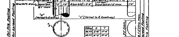
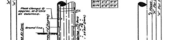
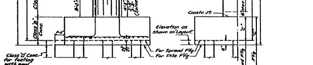
94 Figure Intermediate Bent Cross Section 59

95 Figure Cross Section of Cross Beam Each crossbeam also has two end bent interior girder stops per bent and four intermediate bent girder stops per bent. The end bent interior girder stops are located at the inside face of the girders, while the intermediate bent girder stops are located between girders. See Figure The deck and crossbeams provide a very stiff superstructure, much stiffer than the supporting columns. The three interior bent columns are all supported on spread footings. These columns have clear heights of approximately 24 feet. They have a centerline spacing of 11.3 feet in the lateral direction. Compacted fill surrounds the columns at a height of 60

96 approximately 4 feet from the column base. All of the columns are circular with a diameter of 36 inches. They are reinforced longitudinally with eleven No. 11 reinforcing bars that are spaced evenly around the cross-section perimeter with a clear cover of two inches. Figure Girder Stop Details 61

97 The longitudinal bars extend into the crossbeam without a splice. This provides a l ongitudinal reinforcement ratio of 1.68%. Lap splices of 50 inches (35 longitudinal bar diameters) were used at the bases of the columns. The columns are reinforced in the transverse direction with No. 3 bars spaced every 12 inches. The hoops have an overlap of 21 inches and have no hooks. The transverse reinforcement ratio is 0.14%, which is very small compared to today s standards. This small transverse-reinforcing ratio, combined with a lap splice of this length, has been proven to be a problem in the past. A plastic hinge will form at the base of the column and the splice will breakdown during a major earthquake (Zhang, 1996). The spread footings are 15 feet by 18 feet in the plan view and are 2 feet 3 inches thick. They are reinforced in the bottom layer with 25 No. 10 bars in the 15-foot dimension and 29 No. 9 bars in the 18-foot dimension. The columns are tied into the footing with 90 ο angles on the bottoms. The concrete used in the footings and abutment walls is a WSDOT Class B mix with a compressive strength of f c = 3000 psi. All other concrete used in the bridge, besides that used for the prestressed girders, is a WSDOT Class A mix with a compressive strength of f c = 4000 psi. The steel used in this bridge is Grade 40 with a yield strength of f y = 40,000 psi. 62

98 4.1.3 Structural Model A representation of the bridge model used in this study is shown in Figure and Figure The longitudinal beam and the crossbeams are modeled as very stiff beams. The longitudinal beam can be considered almost rigid because the deck and I- girders are composite, which creates a very stiff superstructure. The crossbeam is much stiffer than the columns so it can also be considered almost rigid. By having a very stiff crossbeam, the load from the longitudinal beam is evenly distributed between the columns, which helps to get the correct axial force in the columns. The columns are modeled with nonlinear beam-column elements. All members are given an appropriate cross-sectional area and mass density so as to model the mass and stiffness correctly. Figure Structural Model of Bridge 5/518 63

99 Figure Bent from Structural Model Because cracking will occur, the effective moment of inertia, I eff, should be used. The effective moment of inertia was determined by using the cross sectional analysis program MPHI2C, developed by Marsh (1991). By plotting the moment versus curvature that is given from MPHI2C, the effective stiffness can be computed by taking a bilinear representation of the plot. (see Figure 4.1-9) The slope of the first line of the bilinear representation gives the effective EI value and by knowing E, the effective moment of inertia can be specified. A preliminary value of I eff, the traditional value of ½ I gross, was used, but it was found to be too stiff compared to the actual tests by Stapleton (2004). Therefore the stiffness, EI, was matched to the actual test by Stapleton (2004), and I eff was found to be approximately ¼ I gross. This value was used in all of the analyses. This is also 64

100 comparable to the I eff values suggested in Figure by Priestley (2003), when the axial load ratio is approximately 0.06 and ρ 1 is approximately The parameters needed by WSU-NEABS to define the axial force-moment interaction curve were also found using MPHI2C. A summary of the structural properties of the longitudinal beam, crossbeam, and columns is shown in Table and Table Moment (k-in) Curvature (1/in.) MPHI2C 1/2 I gross 1/4 I gross Figure Bilinear Representation of Moment-Curvature Table Structural Properties for Columns, Crossbeams, and Deck Beams Young s Modulus (ksi) Poisson Ratio Unit Weight (kips / in 3 ) Axial Area (in 2 ) Shear Area (in 2 ) Bending Inertia (in 4 ) Torsional Inertia (in 4 ) Columns E Crossbeam E E E+7 Deck Beam E E E+7 65

101 Table Yield Function Constants for the Columns M z0 (k in) P 0 (kips) P t / P 0 a 0 a 1 a 2 a Figure Effective Stiffness of Circular Bridge Columns (Priestley, 2003) A boundary spring was used to consider the influence of soil-structure interaction. Table gives the soil stiffness properties for the six degrees of freedom considered for the spring. Springs were attached to all columns and the two abutments. The soil stiffness properties for the abutment springs were computed using the Caltrans seismic design criteria (Caltrans, 2004). The soil stiffness properties for the column supports were computed using WSDOT Bridge Design Manual (WSDOT, 2002). 66

102 Table Stiffness Properties for Soil Springs (k/in) Location Translation X Translation Y Translation Z Rotation X Rotation Y Rotation Z West E+7 1.0E E+6 Abutment Pier Pier Pier East Abutment E+7 1.0E E+6 Rayleigh damping is used in NEABS, where [C] = α[m] + β[k]. In this formulation, α and β are constants and this allows for a linear combination of the system mass matrix [M] and the stiffness matrix [k] to solve for the damping matrix [C]. The two damping factors, α and β, are found by: α 2ξ = β ω i + ω j ω i ω j 1 (4.1) where ω i and ω j are two control natural frequencies and ξ is the damping ratio. It must also be assumed that the two control frequencies have the same damping ratio for this formulation to work. Typically, ω i is the fundamental natural frequency and ω j is set to capture 90 95% mass participation. For reasons of simplification, it is assumed that the fundamental natural frequency controls the dynamic response of the structure. Therefore ω i = ω j = ω and the above equation becomes: 67

103 α ω = ξ 1 β ω (4.2) The natural period was calculated assuming that the columns were fixed at their bases and that they remained elastic. The damping factors were found using this natural frequency and the assumption that the damping ratio was 5%. Idealized expansion joint elements, as seen in Figure and Figure , were used at each of the two abutments and at each pier. Each abutment expansion joint was idealized with one expansion joint element. The expansion joint element accounted for the stiffness in all six degrees of freedom. The expansion joints at the piers were idealized using three separate expansion joint elements. See Figure Figure Idealized Expansion Joint 68

104 Figure Expansion Joint Coordinate System Element number one and number two provide the support between the longitudinal deck beam and the column crossbeam. These elements modeled the effects of the bearing pads and provided for vertical support and relative movements between the crossbeam and the deck beam. The third element in the figure spans between the two deck beams and accounts for the increased stiffness when the gap closes between the deck beams. The impact spring used in element three was assumed to have the axial stiffnes s of the superstructure. The nonlinear properties that were used for modeling the idealized expansion joint are tabulated in Table

105 Figure Idealized Expansion Joints at Intermediate Piers Table Input Parameters for Expansion Joints Support Impacting Hinge Bearing Type Bearing Pad NA Element Width (in.), d Skew (degrees) Impacting Spring Stiffness (kips/in.), k I 2.21 x 10 4 Bearing Friction Stiffness (kips/in.), k F Coefficient of Friction of Bearing, c F 0.02 Stiffness of Tie Bar (kips/in.), k T NA NA Tie Bar Yield Force (kips), Y T NA NA Tie Bar Gap (in.), G T NA NA Seat Gap (in.), G S 1.50 Number of Tie Bars 0 0 Vertical Stiffness (kips/in.), k 3, k 6 x 10 7 Longitudinal Stiffness (kips/in.), k 1, k Transverse Stiffness (kips/in.), k Rotational Stiffness (kips/in.), k 5 70

106 4.1.4 Seismic Excitation A suite of ten earthquakes was used in the time-history analysis. Six of these earthquakes were long-duration events while the other four were short-duration events. Because there are no records of large inter-plate subduction zone earthquakes in Western Washington State, two earthquake records from South American inter-plate subduction zone earthquakes were used. The two earthquakes were the 1985 Llolleo, Chile earthquake record (M = 7.9) and the 2001 Moquegua, Peru earthquake record (M = 8.4). These earthquake records were modified to fit a target acceleration spectrum for Western Washington State. Three attenuation relationships were reviewed by Stapleton (2004); Youngs et al (1997), Atkinson and Boore (2003), and Gregor et al (2002). Figure shows the 5% damped acceleration spectrum for each of the three attenuation relationships. The spectra shown in this figure have been linearly scaled by a factor of two to develop a record that would emulate an extreme event and create damage in the bridge columns. Gregor et al (2002) predicts low spectral accelerations for periods from 0 to 1 seconds and high spectral accelerations beyond 1.5 seconds. Youngs et al (1997) may over estimate the peak spectral acceleration because it lacks a near-source saturation term (Stapleton, 2004). After reviewing the three different attenuation relationships, the Atkinson and Boore (2003) relationship was chosen for use as the target spectrum. Figure shows the target acceleration spectrum, the original acceleration spectrum of the East-West ground motions of the 2001 Peru Earthquake, and the modified spectrum of the Peru Earthquake. Figure shows the entire modified time history of the E-W Peru Earthquake record. The earthquake record duration has been bracketed from the first cycle greater than 0.05g to the last cycle greater than 0.05g. 71

107 Figures and Figure show the North-South acceleration spectra and the modified and bracketed time history for the N-S 2001 Peru Earthquake. The same was done for the 1985 Chile Earthquake. Figures through show the show the spectral acceleration and the modified and bracketed time histories for the Chile E-W and N-S records. These modified earthquakes account for two of the earthquakes in the suite of ten. The time histories from the unscaled acceleration spectra for both earthquakes were also used to account for two more of the earthquakes in the suite. Figure Acceleration Spectra Developed from Attenuation Relationships (Stapleton 2004) 72

108 Figure E-W Peru Spectral Acceleration (Stapleton 2004) Figure Modified Peru Earthquake, E-W Time History (Stapleton 2004) 73

109 Figure N-S Peru Spectral Acceleration (Stapleton 2004) Figure Modified Peru Earthquake, N-S Time History (Stapleton 2004) 74

110 Figure E-W Chile Spectral Acceleration adapted from Stapleton (2004) Figure Modified Chile Earthquake, E-W Time History (Stapleton 2004) 75

111 Figure N-S Chile Spectral Acceleration (Stapleton 2004) Figure Modified Chile Earthquake, N-S Time History (Stapleton 2004) 76

112 Figures , , and show the target acceleration spectrum used in this study compared with spectra from Frankel et al (1996) for Seattle, Olympia, and Grey s Harbor, WA. The target spectrum is compared with different return period ground motions. The fundamental period of the bridges used in this study are approximately one second. Figure % Damped Spectral Accelerations for Seattle, WA (Frankel, 1996) 77

113 Figure % Damped Spectral Accelerations for Olympia, WA (Frankel, 1996) Figure % Damped Spectral Accelerations for Grey s Harbor, WA (Frankel, 1996) 78

114 The Washington State Department of Transportation (WSDOT) supplied the last six earthquake time histories. All six of these time histories were modified to fit an acceleration spectrum representative of the Seattle area. The six time histories come from three different earthquakes. Each earthquake has time histories that have been scaled for a 475 and a 950 year return period, respectively. The first of these three earthquakes was a long-duration earthquake from the 1985 Mexico City Earthquake. The last two are short-duration earthquake from the 1995 Kobe Earthquake and the 1949 Olympia Earthquake. All of the time histories for these earthquakes can be found in Appendix A. 4.2 WSDOT Bridge 5/826 A second bridge was chosen for this study to help understand the effects of long duration earthquakes on lightly reinforced concrete bridges. The bridge is WSDOT Bridge 5/826 and it was modeled in much the same way as the previous bridge Introduction The bridge shown in Figure is located at milepost on Smith Road in King County of Washington State. It was constructed in 1972 to carry Smith Road over Interstate 5. This bridge is also a lightly reinforced bridge as well as having splices in the plastic hinge region. 79

115 Figure Bridge 5/ Description of the Bridge The plan and elevation of the bridge are shown in Figures and The bridge is 369 feet long and has four spans. The two middle spans are both 121 feet long, while the two end spans are 57 and 70 feet long, respectively. The reinforced concrete deck, which provides the main transverse stiffness of the super structure, is continuous at all interior supports. It is 40 feet wide and has a thickness of 7.0 inches. The deck is supported by six prestressed concrete I-girders that are 6 feet 1.5 inches deep. These I- girders are spaced at 7 feet 4 inches on center. The I-girders rest on the abutments on top of a grout pad topped with a 2.5 inch laminated elastomeric bearing pad. At the intermediate piers, the I-girders are cast into the crossbeam, which provides a very stiff superstructure. The provided superstructure is then much stiffer than the supporting columns. 80

116 Figure Plan V iew of Bridge 5/826 Figure Elevation View of Bridge 5/826 The crossbeam was cast monolithically with the three columns at each bent. The crossbeam has a total length of 50 feet 2.25 inches, a width of 48 inches, and a depth of 6 feet 11 inches. See Figure The crossbeams at piers No. two and four are reinforced with ten No. 10 bars at the top and eight No. 8 bars in the bottom. Pier No. 3 is reinforced with ten No. 10 bars in the top and eight No. 9 bars in the bottom. All piers also have eight No. 6 reinforcing bars along each side of the crossbeam. An inner and 81

117 outer reinforcing hoop provided confinement. The hoops are No. 5 reinforcing bars at varying spacing along the length of the crossbeam to account for shear. All nine of the columns at the interior bents are supported on pile caps placed on top of driven piles. The columns have clear heights of 23.5 feet at pier No. 2, 22 feet at pier No. 3, and 24.5 feet at pier No. 4. They have a centerline spacing of 19.5 feet in the lateral direction. Compacted fill surrounds the columns to a height of approximately 4 feet. All of the columns are circular with diameters of 36 inches. They are reinforced longitudinally with seventeen No. 11 reinforcing bars that are evenly spaced around the cross-section perimeter with a clear cover of 1.5 inches. The longitudinal bars extend into the crossbeam without a splice. Figure Cross Section of Cross Beam of Bridge 5/826 The columns have a longitudinal reinforcement of 2.6%. Lap splices of 63 inches were used at the base of the columns. The columns are reinforced in the transverse direction with No. 4 bars spaced every 6 inches. The hoops have an overlap of 24 inches 82

118 and have no hooks. The transverse reinforcement ratio is 0.4%. All column details are shown in Figure Figure Column Cross Section of Bridge 5/826 Each column is on a separate foundation consisting of a pile cap that is cast monolithically with the column. The pile caps are all 12 feet 9 inches square in the plan view and 3 feet 6 inches thick. The pile caps at Pier No. 3 are supported on 16 treated 83

119 timber piles. There are four rows of four piles with centerline spacings of 3 feet 3 inches. The pile caps at piers 2 and 4 are supported on 14 driven piles. There are four rows with three piles in the first and fourth rows and four piles in the middle two rows. See Figure The pile caps contain two mats of steel placed in the top and bottom of the elevation. The mat at the top consists of No. 5 bars running in both directions, spaced every 6 inches for the pile caps at all piers. The mat in the bottom of the pile caps at piers 2 and 4 consists of No. 8 bars running in both directions, spaced every 6 inches. The mat in the bottom of the pile caps at pier No. 3 consists of No. 9 bars running in both directions, spaced every 6 inches. Figure Column Footing Plans for Bridge 5/826 The abutments are set on driven piles. The pile caps at the abutments are 6 feet 3 inches by 56 feet 6.5 inches in the plan view, and they are 2 feet thick. The pile caps are 84

120 supported on 20 treated timber driven piles. There are 10 rows of two piles each, along the length of the abutment. See Figure for the abutment details. The pile cap has two mats of steel located at the top and bottom with clear covers of 2 inches at the top and 2.5 inches at the bottom. The steel mats consist of No. 6 bars running in both directions, spaced at 12 inches. The abutment pile caps are cast monolithically with the abutment walls and have two No. 5 bars spaced every foot, running up into the wall. Figure Abutment Footing Plan for Bridge 5/826 The concrete used in the pile caps and abutment walls is a WSDO T Class B mix with a compressive strength of f c = 3000 psi. All other concrete used in the bridge, besides that used for the prestressed girders, is a WSDOT Class AX mix with a compressive strength of f c = 4000 psi. The reinforcing steel used in this bridge is Grade 40 with a yield strength of f y = 40,000 psi. 85

121 4.2.3 Structural Model A drawing of the bridge model used in this study is shown in Figure The longitudinal deck beams and the crossbeams are modeled as very stiff beams. Like Bridge 5/518, the longitudinal beam can be considered almost rigid because of the composite action of the deck and I-girders. Because the crossbeam is much stiffer than the columns, it can be considered almost rigid as well. The columns are modeled with nonlinear beam-column elements and are given an appropriate cross sectional area and mass density. A summary of the structural properties of the longitudinal deck beam, crossbeams, and columns is shown in Table and Table Figure Structural Model of Bridge 5/826 86

122 Table Structural Properties for Columns and Crossbeams Young s Modulus (ksi) Poisson Ratio Unit Weight (kips / in 3 ) Axial Area (in 2 ) Shear Area (in 2 ) Bending Inertia (in 4 ) Torsional Inertia (in 4 ) Columns E Crossbeam E E+6 Deck Beam E E+8 0E+8 Table Yield Function Constants for the Columns M z0 (k in) P 0 (kips) P t / P0 a0 a1 a2 a Boundary springs are used to consider the influence of soil-structure interaction. The soil stiffness properties for the six degrees of freedom are listed in Table Springs were attached at all columns and the two abutments. The soil stiffness properties were obtained using the WSDOT Bridge Design Manual (WSDOT, 2002). Table Stiffness Properties for Soil Springs (k/in) Location Translation X Translation Y Translation Z Rotation X Rotation Y Rotation Z West E+7 E+7 E+8 Abutment Pier E+8 Pier E+8 Pier E+8 East Abutment E+7 E+7 E+8 87

123 Rayleigh damping was used for this bridge model and coefficient values were assigned as was previously explained in section Because the deck of this bridge is continuous, expansion joints were only needed at the two abutments. Each abutment expansion joint was idealized with one expansion joint element. The expansion joint element accounted for the stiffness in all six degrees of freedom. The expansion joint element allows for a 1.5 inch seat gap and has an impact spring that accounts for the increased stiffness when the gap closes. This impact spring was assumed to have the same axial stiffness as the longitudinal deck beam. The nonlinear properties of the expansion joints are tabulated in Table Table Input Parameters for Expansion Joints Support Impacting Hinge Bearing Type Bearing Pad NA Element Width (in.), d Skew (degrees) Impacting Spring Stiffness (kips/in.), k I 2.21 x 10 4 Bearing Friction Stiffness (kips/in.), k F Coefficient of Friction of Bearing, c F 0.02 Stiffness of Tie Bar (kips/in.), k T NA NA Tie Bar Yield Force (kips), Y T NA NA Tie Bar Gap (in.), G T NA NA Seat Gap (in.), G S 1.50 Number of Tie Bars 0 0 Vertical Stiffness (kips/in.), k 3, k 6 x 10 7 Longitudinal Stiffness (kips/in.), k 1, k Transverse Stiffness (kips/in.), k Rotational Stiffness (kips/in.), k Seismic Excitation The same seismic excitation was used for this bridge as was used on Bridge 5/

124 Chapter 5 Analytical Results and Interpretation 5.1 Introduction Presented in this chapter are selected time history analysis results from the nonlinear finite element analysis of WSDOT Bridges 5/518 and 5/826. The results include the displacement at the top of the piers, the plastic rotation of the plastic hinges at the top of the columns, the damage corresponding to the plastic rotation found in the plastic hinges, column moment, column shear, and displacement of the expansion joints. 5.2 Bridge 5/518 The results from analyses using the modified Peru and modified Chile earthquakes and the model of Bridge 5/518 are presented here. These two cases were chosen because they are the two extreme cases, and they show the most information about the response of the bridge with respect to the new damage model Modified Peru Earthquake Figures through show the total displacement time histories at the top of the intermediate piers, where relative displacement is the difference between displacement at the top versus that at the column base. The total relative displacement was found by taking the square root of the sum of the squares of the longitudinal and transverse displacem ents. The figures show that the total relative displacements at the center pier are much larger than those of the outer piers. This can be seen by looking at the displacement envelope shown in Figure 5.2-4, where the maximum relative transverse 89

125 displacements at each pier are plotted. The greater displacement at the center pier is not surprising since the abutments provide some restraint in the transverse direction. The figure also shows that most of the displacement is in the transverse direction. This is because the period of the bridge in the transverse direction is much greater than it is in the lon gitudinal direction. The longitudinal displacements are similar for all three piers because the deck is virtually rigid compared to the columns Figure Total Relative Displacement at Pier 1, Modified Peru Earthquake 90

126 Time (sec.) Figure Total Relative Displacement at Pier 2, Modified Peru Earthquake Time (sec.) Figure Total Relative Displacement at Intermediate Pier 3, Modified Peru Earthquake 91

127 Pier Pier 1 Pier Distance Along Bridge (in.) Figure Transverse Displacement Envelope of Bridge Deck, Modified Peru Earthquake Because the foundation springs at the bottom of every column allowed for slight rotations, the plastic rotation was confined to plastic hinges at the top of the columns. Table shows the maximum moments at the top and bottom of all of the columns. It should be noted that yielding limits the amount of moment that can be developed in the columns, and the yield level depends on the level of axial force. 92

128 Table Maximum Moment (kip-in) at the Top and Bottoms of Columns, Modified Peru Earthquake Moment Pier No. Column Top Bottom Because the displacements at the center pier were larger then those at the outer piers, the plastic rotations in the plastic hinges found in that pier were larger, as shown in Figure Pier 1 and Pier 3 are the outer piers, and the center pier is Pier 2. It should also be noted that the columns in the center pier have many more plastic rotation cycles then the columns of the other piers Pier 1 - Outer Pier 1 - Center Pier 1 - Outer Pier 2 - Outer Pier 2 - Center Pier 2 - Outer Pier 3 - Outer Pier 3 - Center Pier 3 - Outer Plastic Ro tatio n (rad) Time (sec.) Figure Plastic Rotations at the T op of the Columns, Modified Peru Earthquake 93

129 D ue to the fac t that the columns in the center pier experienced larger plastic rotations and more plastic rotation cycles than those of the outer piers, the columns in the center pier also accumulated more damage, as shown in Figure The levels of damage in the columns at Pier 1 are less than those of the columns at Pier 3. This is due to the fact that the span that connects to Pier 1 is the shorter of the two end spans, and therefore allows for less displacement. 3.00E-01 Pier 1 - Outer Pier 1 - Center Pier 1 - Outer Pier 2 - Outer Pier 2 - Center Pier 2 - Outer Pier 3 - Outer Pier 3 - Center Pier 3 - Outer 2.50E-01 E-01 Damage 1.50E-01 E E-02 E Time (sec.) Figure Damage at the Top of the Columns, Modified Peru Earthquake The damage coefficients for the columns at the center pier ranged in value between 0.14 and 0.23, which would indicate that there is light cracking throughout the column section. The damage coefficients in the columns at the other piers are at or below 0.05, which would suggest only minor cracking. The indicated damage is small enough that localized spalling would not occur. By looking at the shear versus displacement hysteresis plots, as shown in Figures and 5.2-8, it can also be seen that the demand 94

130 on the columns is not very large. In the longitudinal direction, the hysteresis loops only open slightly, which would suggest that there was only minor yielding. The hysteresis loops for the transverse direction open more, but they also show little significant yielding, which is consistent with the accumulated damage. Figure also shows that, as the damage accumulated and the hysteresis loops opened, the stiffness was reduced (k) Shear Figure Longitudinal Hysteresis Plot for the Center Column of Pier 2, Modified Peru Earthquake 95

131 Shear (k) Figure Transverse Hysteresis Plot for the Center Column of Pier 2, Modified Peru Earthquake The maximum shear values at the top and bottom of the columns are shown in Table The shear values are different at the top and bottom because the soil spring at the base of the column allows for some column rotation, which causes a variation in local force components. The shear capacity of the columns was based solely on the concrete for simplicity and was determined according to Kowalsky and Priestley (2000): V = 2.8 f ' c * c A e where A e is taken as 80% of the gross area of the column and f c was taken as 6000 psi. The specification for the bridge requires f c = 4000 psi, but Priestley (1996) recommends using 1.5* f c as being more representative of the actual concrete strength in older bridges. This gives a final shear capacity of kips for the columns. Since the maximum shear in the columns was 128 kips, the shear capacity was not exceeded. 96

132 Columns with smaller aspect ratios than those that are found in this bridge should be investigated further. Table Maximum Shear (kips) in the Columns, Modified Peru Earthquake Shear Pier No. Column Top Demand/ Capacity Bottom Demand/ Capacity The maximum abutment forces in the transverse and longitudinal directions are found in Table The shear capacity of the abutments was determined according to the AASHTO Brid ge Design Specifications (AASHTO, 1998), where the nominal shear strength is calculated by: V 0. 2 f ' n c A cv where A cv is the area of the concrete engaged in shear transfer. The value of A cv in the longitudinal direction for this bridge is 3744 in 2, which incorporates the cross section of the thinnest portion of the abutment wall. This gives a nominal shear capacity of 3370 kips. The shear forces in the abutments in the longitudinal direction were not near the 97

133 capacity limit, therefore the abutment is considered capable of resisting the seismic demands. The value of A cv in the transverse direction for this bridge is 1620 in 2, which incorporates the cross section of the girder stops along the crossbeam. This gives a nominal shear capacity of 1458 kips. This is also much greater than the actual force seen by the abutment in the analysis. Table Maximum Shear (kips) at the Abutments, Modified Peru Earthquake Shear Abutment Longitudinal Demand/ Transverse Demand/ Capacity Capacity West East By looking at the relative longitudinal displacement of the expansion joints, it can be determined if there will be pounding at the abutments and piers. Figure shows the relative longitudinal displacement at the West abutment. It should be noted that when the relative displacement is negative, the expansion joint is closing. The expansion joint has a gap of 1.5 inches, so it can be seen that pounding occurs at the West abutment. Pounding occurs at all of the piers and at the other abutment, as well. The plots for the other abutment and piers can be found in Appendix C. It was within the scope of this project to determine if pounding occurs but not to quantify the damage due to pounding. Further research should be done to determine those effects. 98

134 Gap Closed Figu re Relative Longitudinal Displacement at the West Abutment, Modified Peru Earthquake The maximum displacement that the bearing pads can withst and was determined by the equation (Priestley, 1996): x b = hγ s where h is the thickness of the bearing pad and γ s is the allowable shear strain. The maximum shear strain, γ s, is taken conservatively as: γ s = 0. 2ε tu where ε tu is the failure tensile strain. An average ε tu value of 5.75 was assumed (Priestley, 1996), and the thickness of the bearing pad is 1.25 inches. This gives an 99

135 allowable displacement of 1.44 inches while the actual displacement is predicted to be 2.72 inches. It shou ld be noted that conservative valu es have been used, but they imply that a failure of the beari ng pad could occur. After such a large earth quake, the bridge appears to be in good condition. The columns do not accumulate excessive damage and they are capable of resisting the shear demands. The abutments are also able to resist the shear demands in both the longitudinal and transverse directions. The two main concerns would be the pounding of the expansion joints that occurs at the abutments and piers and a possible failure of the bearing pads Modified Chile Earthquake Figures through show the relative displacement time histories at the top of the intermediate piers. The figures show that the total relative displacements at the center pier are much larger than those of the outer piers. This can be seen by looking at the transverse displacement envelope shown in Figure The figure also shows that most of the displacement is in the transverse direction. This is because the period of the bridge in the transverse direction is much greater than it is in the longitudinal direction. 100

136 Figure Total Relative Displacement at Pier 1, Modified Chile Earthquake Time (sec.) Figure Total Relative Displacement at Pier 2, Modified Chile Earthquake 101

137 Time (sec.) Figure Total Relative Displacement at Pier 3, Modified Chile Earthquake Pier Pier 1 Pier Distance Along Bridge (in.) Figure Transverse Relative Displacement Envelope of Bridge Deck, Modified Chile Earthquake 102

138 Because the foundation springs at the base of every column allow for slight rotations, the plastic rotation was confined to the plastic hinges at the top of the columns. Table shows the maximum moments at the top and bottom of all the columns. Table Maximum Moment (kip-in) at the Top and Bottoms of Columns, Modified Chile Earthquake Moment Pier No. Column Top Bottom Because the displacements at the center pier were larger then those at the outer piers, the plastic rotations in the plastic hinges found in that pier were larger, as shown in Figure The columns in the center pier also have more plastic rotation cycles than do the other piers, which causes more damage. 103

139 0.012 Pier 1 - Outer Pier 1 - Center Pier 1 - Outer Pier 2 - Outer Pier 2 - Center Pier 2 - Outer Pier 3 - Outer Pier 3 - Center Pier 3 - Outer 7 Plastic Rotation (rad) Time (sec.) Figure Plastic Rotations at the Top of the Columns, Modified Chile Earthquake Due to the fact that the columns in the center pier experienced larger plastic rotations and more plastic rotation cycles, the columns in the center pier accumulated the most damage as shown in Figure

140 2.20E-01 Pier 1 - Outer Pier 1 - Center Pier 1 - Outer Pier 2 - Outer Pier 2 - Center Pier 2 - Outer Pier 3 - Outer Pier 3 - Center Pier 3 - Outer 1.70E-01 Damage 1.20E E-02 E E-02 Time (sec.) Figure Damage at the Top of the Columns, Modified Chile Earthquake The damage coefficients for the columns at the center pier and an outer column at Pier 3 ranged in value between and 0.094, which indicates that there is anywhere from localized minor cracking to light cracking throughout the column section. The d amage coefficients in all of the other columns are at or below 0.03, which would suggest negligible cracking. It should be noted that all columns had damage, although the figure only shows traces for eight of the nine columns. The center column of Pier 1 plots underneath other columns, with damage levels of about All indicated damage levels are small enough that localized spalling would not occur. Figure shows the estimated damage that would be seen in the columns. This picture was taken after the modified Chile displacement record was applied to the test specimen from the testing done by Stapleton (2004). It shows very little damage. 105

141 Figure Final State of Damage in Column By looking at the shear versus displacement hysteresis plots, as shown in Figure and , it can also be seen that the demand on the columns is not very large. In the longitudinal direction, the hysteresis loops only open slightly, which would suggest that there was only minor yielding. The hysteresis loops for the transverse direction open more, but they also sho w little significant yield ing, which is consistent with the accumulated damage. 106