Chapter 2 Time-Domain Representations of LTI Systems

Size: px

Start display at page:

Download "Chapter 2 Time-Domain Representations of LTI Systems"

Felicity Martin
5 years ago
Views:

1 Chapter 2 Time-Domain Representations of LTI Systems 1 Introduction Impulse responses of LTI systems Linear constant-coefficients differential or difference equations of LTI systems Block diagram representations of LTI systems State-variable descriptions for LTI systems Summary

2 Contents 2 Introduction Convolution Sum Convolution Sum Evaluation Procedure Convolution Integral Convolution Integral Evaluation Procedure Interconnection of LTI Systemss Relations between LTI System Properties and the Impulse Response Step Response

3 1. Contents (c.1) 3 Differential and Difference Equation Representations of LTI Systems Solving Differential and Difference Equations Characteristics of Systems Described by Differential and Difference Equations Block Diagram Representations State-Variable Descriptions of LTI Systems. Exploring Concepts woth MatLab

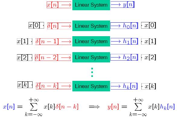
4 2. Convolution Sum 4 An arbitrary signal is expressed as a weighted superposition of shifted impulses. x n x k n k k Input x[n] LTI system H Output y[n]

5 5 2. Convolution Sum Convolution Impulse Response of the System H [ x ( n )] H [ x ( k ) ( n k )] x ( k ) H [ ( n k )] x ( k ) h ( n k ) k k k x n h n x k h n k k

6 2. Convolution Sum 6

7 7 2. Convolution Sum

8 2. Convolution Sum 8 Example 2.1 Multipath Communication Channel: Direct Evaluation of the Convolution Sum Consider the discrete-time LTI system model representing a two-path propagation channel described in Section If the strength of the indirect path is a = ½, then 1 yn xn xn 1 2 Letting x[n] = [n], we find that the impulse response is h n 1, n 0 1, n 1 2 0, otherwise xn 2, n 0 4, n 1 2, n 2 0, otherwise

9 2. Convolution Sum 9 <Sol.> 1. Input: xn 2 n 4 n 1 2 n 2 2. Since time-shifted impulse input [n k] 3. Output: y n h n h n h n Input = 0 for n < 0 and n > 0 time-shifted impulse response output h [n k] yn 0, n 0 2, n 0 5, n 1 0, n 2 1, n 3 0, n 4

10 10 3. Convolution Sum Evaluation Procedure Define intermediate signal k = independent variable n [k] x[k]h[n k] y n x k h n k n is treated as a constant by writing n as a subscript on w. h [n k] = h [ (k n)] is a reflected (because of k) and time-shifted (by n) version of h [k]. Since y[n] n[k] k The time shift n determines the time at which we evaluate the output of the system. k

11 11 3. Convolution Sum Evaluation Procedure

12 3. Convolution Sum Evaluation 12 Procedure Procedure (reflect and shift convolution sum evaluation) Step 1: Time-reverse (reflect): h[k] h[-k] Step 2: Choose an n value and shift h[.] by n: h[n-k]. Step 3: Compute wn[k] = x[k]h[n-k] Step 4: Summation over k: y[n]=σk wn[k] Step 5: Choose another n value, go to Step 2. Step 6: Slide a window of h[k] over the input signal from left to right.

13 13 3. Convolution Sum Evaluation Procedure Check values in y[n]

14 4. Convolution Integral 14 The output of a continuous-time (CT) LTI system may also be determined solely from knowledge of the input and the system s impulse response. Signal Integral x(t) x( ) (t - )d Linear System - Shift-Invariance y t H x t H x t d y(t) - - x( )H{ (t - )}d y(t) x( )h(t )d H{ (t - )} h(t - )

15 4. Convolution Integral 15 Convolution Operator

16 16 5. Convolution Integral Evaluation Procedure Define the immediate signal t w x h t Evaluate the output signal at a specific time t y(t) w t( )d -

17 6. Interconnection of LTI Systems 17 Relationships between the impulse response of an interconnection of LTI system and the impulse responses of the constituent systems. y( t) y ( t) y ( t) 1 2 x( t) h ( t) x( t) h ( t) 1 2 y( t) x( ) h ( t ) d x( ) h ( t ) d 1 2 y( t) x( ) h ( t ) h ( t ) d 1 2 x( ) h( t ) d x( t) h( t) x(t) h (t) x(t) h (t) x(t) {h (t) h (t)} x[n] * h1[n] + x[n] * h2[n] = x[n] * {h1[n] + h2[n]}

18 6. Interconnection 18 of LTI Systems Cascade y(t) = z(t) * h2(t) = {x(t) * h1(t)} * h2(t)

19 6. Interconnection of LTI Systems 19 Communicative y[ k] h[ k i] u[ i] h[ k]* u[ k] i h[ i] u[ k i] u[ k]* h[ k] i Parallel Sum x[ n]*{ h [ n] h [ n]} 1 2 x[ n]* h [ n] x[ n]* h [ n] 1 2 x[n] h[n] x[n] x[n] y[n] h[n] y[n] x[n] y[n] h1[n]+h2[n] y[n] h1[n] + h2[n] Cascade Form x[ n]*{ h 1 { x[ n]* h [ n]* h 1 2 [ n]} [ n]}* h 2 [ n] x[n] h1[n] h2[n] y[n] x[n] y[n] h1[n]*h2[n]

20 6. Interconnection of LTI Systems 20 x( t) h ( t) h ( t) x( t) h ( t) h ( t), h (t) h (t) h (t) h (t) {x[n] h 1[n]} h 2[n] x[n] {h 1[n] h 2[n]} h [n] h [n] h [n] h [n]

21 21 6. Interconnection of LTI Systems

22 22 7. Relations between LTI System Properties and the Impulse Response Memoryless Systems Discrete-Time Systems y[ n] h[ n] x[ n] h[ k] x[ n k] h( ) c ( ) k Continuous-Time Systems h[ k] c [ k]

23 23 7. Relations between LTI System Properties and the Impulse Response Causal Systems h[ k] 0 for k 0 h( ) 0 for 0

24 24 7. Relations between LTI System Properties and the Impulse Response Stable LTI Systems DT x[ n] M x Output: y[ n] M y y[ n] h[ n] x[ n] h[ k] x[ n k] k y[ n] h[ k] x[ n k] a b a b k y[ n] h[ k] x[ n k] k x[ n] M x y[n] Mx h[k] k hk [ ]. BIBO k ab a b The impulse response is absolutely summable is both sufficient and necessary condition.

25 25 7. Relations between LTI System Properties and the Impulse Response Stability of LTI Systems (BIBO, Bounded-Input-Bounded Output System) Linear time-invariant systems are stable if and only if the impulse response is absolutely summable, i.e., if <pf> Since that S y[ n] k h[ k ] k If x[n] is bounded so that then k h[ k] h[ k] x[ n k] x[ n k] y [ n ] B h[ k ] x k x [ n ] B x If S= x [ n ] then the bounded input will generate h *[ n ] h n h[ n ], [ ] 0 0, h[ n ] 0 h[ k ] y [ 0] x [ k ] h[ k ] S h[ k ] k k 2

26 26 7. Relations between LTI System Properties and the Impulse Response Similarly, a continuous-time LTI system is BIBO stable if and only if the impulse response is absolutely integrable 0 h( ) d. Example 2.12 Properties of the First-Order Recursive System The first-order system is described by the difference equation y[ n] y[ n 1] x[ n] and has the impulse response n h[ n] u[ n] Is this system causal, memoryless, and BIBO stable? <Sol.> 1. The system is causal, since h[n] = 0 for n < The system is not memoryless, since h[n] 0 for n > Stability: Checking whether the impulse response is absolutely summable?

27 7. Relations between LTI System 27 Properties and the Impulse Response A system is invertible If the input to the system can be recovered from the output except for a constant scale factor. The existence of an inverse system that takes the output of the original system as its input and produces the input of the original system. x(t) * (h(t) * hinv(t))= x(t). h(t) * hinv(t) = δ(t) Similarly, h[n] * hinv[n] = δ[n]

28 28 7. Relations between LTI System Properties and the Impulse Response Example 2.13 Multipath Communication Channels: Compensation by means of an Inverse System Consider designing a discrete-time inverse system to eliminate the distortion associated with multipath propagation in a data transmission problem. Assume that a discrete-time model for a two-path communication channel is y[ n] x[ n] ax[ n 1]. Find a causal inverse system that recovers x[n] from y[n]. Check whether this inverse system is stable. <Sol.> 1. Impulse response: 1, n 0 h[ n] a, n 1 0, otherwise 2. The inverse system h inv [n] must satisfy h[n] h inv [n] = [n]. inv inv h [ n] ah [ n 1] [ n].

29 29 7. Relations between LTI System Properties and the Impulse Response 1) For n < 0, we must have h inv [n] = 0 in order to obtain a causal inverse system 2) For n = 0, [n] = 1, and eq. (2.32) implies that inv inv h [ n] ah [ n 1] 0, inv inv h [n] ah [n 1] (2.33) 3. Since h inv [0] = 1, Eq. (2.33) implies that h inv [1] = a, h inv [2] = a 2, h inv [3] = a 3, and so on. The inverse system has the impulse response inv n h [ n] ( a) u[ n] 4. To check for stability, we determine whether h inv [n] is absolutely summable, which will be the case if inv k h [ k] a is finite. k k For a < 1, the system is stable.

30 30 7. Relations between LTI System Properties and the Impulse Response

31 8. Step Response 31 Step response is the output due to a unit step input signal Step input signals are often used to characterize the response of an LTI system to sudden changes in the input s[ n] h[ n]* u[ n] h[ k] u[ n k]. k Since u[n k] = 0 for k > n and u[n k] = 1 for k n, we have s[ n] h[ k]. n k h[ n] s[ n] s[ n 1] Similarly for CT system t s(t) h( )d d h( t) s( t) dt

32 8. Step Response 32 Example 2.14 RC Circuit: Step Response The impulse response of the RC circuit depicted in Fig is t 1 RC h( t) e u( t) RC 1. Step respose: st () 1 RC st () 1 RC t t 1 RC s( t) e u( ) d. RC 0, t 0 RC e u( ) d t 0 0, t 0 t RC e d t 0 0, t 0 t RC 1 e, t 0 0

33 33 9. Differential and Difference Equation Representations of LTI Systems Linear constant-coefficient difference and differential equations provide another representation for the inputoutput characteristics of LTI systems. CT: Constant coefficient differential equation N k M k d d a y(t) bk x(t) k dt k k k0 dt k0 DT: Constant coefficient difference equation N a y[n k] b x[n k] M k k0 k0 k The order of the differential or difference equation is (N,M), representing the number of energy storage devices in the system. Often, N>= M, and the order is described using only N.

34 9. Differential and Difference Equation 34 Representations of LTI Systems Example Summing the voltage loop Differentiating both sides The order is N = 2 and the circuit contains two energy storage devices: a capacitor and an inductor.

35 35 9. Differential and Difference Equation Representations of LTI Systems Example of a Difference Equation 1 y[n] y[n 1] y[n 2] x[n] 2x[n 1] 4 Rearrange the equation 1 y[n] x[n] 2x[n 1] y[n 1] y[n 2] 4 Starting from n = 0, compute the current output from the input and the past outputs We must know two most recent past values of the output, namely, y[-1] and y[-2]. These values are called initial conditions.

36 36 9. Differential and Difference Equation Representations of LTI Systems Initial Conditions Summarize all the information about the system s past needed to determine future outputs. In general, the number of initial conditions required to determine the output is equal to the maximum memory of the system. DT: Nth-order difference eqn. N values y[-n], y[-n+1],, y[-1]. CT: Nth-order differential eqn. first N derivatives of the output; that is, 2 N 1 d d d yt yt, yt,..., y t t0, 2 N 1 dt t0 dt t0 dt t0 Note: The textbook says the first N derivatives, which include y(t) t=0-, the 0th-order derivative.

37 Solving Differential and Difference Equations Given x(t) (input), find y (t) (output) y = y (h) + y (p) = homogeneous solution + particular solution Homogeneous solution for Differential Equations N k0 k d ak y t k dt h 0 The homogeneous solution is the solution the form N (h) rt i y (t) cie i0 ci are to be decided in the complete solution and ri are the N roots of the system s characteristic equation N k akr 0 k0

38 Solving Differential and Difference Equations Homogeneous solution for Difference Equation N k0 k h a y n k 0 The homogeneous solution is the solution the form N (h) n y [n] cii r i1 ci are to be decided in the complete solution and ri are the N roots of the system s characteristic equation N Nk akr 0 k0

39 Solving Differential and Difference Equations If a root r j is repeated p times in characteristic eqs., the corresponding solutions are Continuous-time case: Discrete-time case: Example d yt RC yt xt dt d y t RC y t dt 1. Homogeneous Eq.: 0 2. Homo. Sol.: h 1 y t c e rt 1 V r t r t p1 r t e, te,..., t e j j j r, nr,..., n r n n p1 n j j j 3. Characteristic eq.: 1RCr1 0 r 1 = 1/RC 4. Homogeneous solution: t h RC 1 V y t c e

40 Solving Differential and Difference Equations Example 1 y n y n x n 1. Homogeneous Eq.: yn yn 2. Homo. Sol.: h n y n c11 r 3. Characteristic eq.: r Homogeneous solution: 1 0 h 1 n y n c

41 Solving Differential and Difference Equations Particular Solution The particular solution y (p) represents any solution of the differential or difference eqn. for the given input. y (p) is not unique. A particular solution is usually obtained by assuming an output of the same general form as the input yet is independent of all terms in the homogenous solution. Example 1 y n y n x n if the input is x[n] = (1/2) n. 1. Particular solution form: p y [ n] c p 1 2. Substituting y (p) [n] and x[n] into the given difference 1 1 n 1 n 1 n p 1 1 cp c 2 p c 2 2 p(12 ) 1 y n n n

42 Solving Differential and Difference Equations Hypothesis for the Particular Solution

43 Solving Differential and Difference Equations Procedure Procedure 2.3: Solving a Differential or Difference equation 1. Find the form of the homogeneous solution y (h) from the roots of the characteristic equation. 2. Find a particular solution y (p) by assuming that it is of the same form as the input, yet is independent of all terms in the homogeneous solution. 3. Determine the coefficients in the homogeneous solution so that the complete solution y = y (h) + y (p) satisfies the initial conditions.

44 Solving Differential and Difference Equations Example First-Order Recursive System (Continued): Complete Solution Find the complete solution for the first-order recursive system described by the difference equation 1 y[n] y[n 1] x[n] 4 if the input is x[n] = (1/2) n u[n] and the initial condition is y[ 1] = 8. <Sol.> 1. Homogeneous sol.: 4. Coefficient c 1 determined by I.C.: y 0 x y 1 y 0 x 0 (1 4) 8 3 h y n c n 2. Particular solution: y p n n Complete solution: n n y[n] 2( 1 ) c 1 1( ) 2 4 We substitute y[0] = c Final solution: yn n n for n 0 c 1 = 1

45 Solving Differential and Difference Equations 1. Homogeneous sol.: 2. Particular solution: h y t rt c e p 1 RC y t cos 2 t sin 2 t 1 RC 1 RC V 1 1 V 0 = 1 3. Complete solution: R = 1, C = 1 F t 1 1 yt ce cost sint V Coefficient c 1 determined by I.C.: y(0 ) = y(0 + ) y(0 2 ce cos0 sin 0 c c = 3/2 ) = 2 V Final solution: 3 t 1 1 yt e cost sint V x(t) = cos(t)u(t) R = 1 and C = 1 F

46 11. Characteristics of Systems Described 46 by Differential and Difference Equations Natural Response The system output for zero input. It is produced by the stored energy or memory of the past (non-zero initial conditions). Homogeneous solution by choosing the coefficients ci so that the initial conditions are satisfied. It does not involve the particular solution. The natural response is determined without translating initial conditions forward in time.

47 11. Characteristics of Systems Described 47 by Differential and Difference Equations Forced response: the system output due to the input signal assuming zero initial conditions. It has the same form as the complete sol. A system with zero initial conditions is said to be at rest. The atrest (zero state) initial conditions must be translated forward before solving for the undetermined coefficients. DT: y[-n] = y[-n+1] = = y[-1] = 0 y[0], y[1],, y[n -1] CT: Initial conditions at t = 0- t = 0+ We shall only solve the differential eqns. of which initial conditions at t = 0+ are equal to the zero initial conditions at t = 0-.

48 Characteristics of Systems Described by Differential and Difference Equations Find the natural response of the this system, assuming that y(0) = 2 V, R = 1 and C = 1 F. d y t RC y t x t dt 1. Homogeneous sol.: h t y t c1e V 2. I.C.: y(0) = 2 V y (n) (0) = 2 V c 1 = 2 3. Natural Response: n t 2 V y t e

49 11. Characteristics of Systems Described 49 by Differential and Difference Equations Impulse response 1. We do not know the form of particular sol. for impulse input (why?). In general, we can find the step response assuming that the system is at rest. Then, the impulse response is obtained by taking differentiation (CT) or difference (DT) on the step response. Step response is the output due to a unit step input signal 2. Impulse response is obtained under the assumption that the systems are initially at rest or the input is known for all time.

50 11. Characteristics of Systems Described 50 by Differential and Difference Equations Linearity The forced response of an LTI system described by a differential or difference eqn. is linear with respect to theinput (zero I.C.). The natural response of an LTI system described by a differential or difference eqn. is linear with respect to the initial conditions (zero input).

51 11. Characteristics of Systems Described 51 by Differential and Difference Equations Time invariance The forced response of an LTI system described by a differential or difference eqn. is time-invariant. In general, the output (complete sol.) of an LTI system described by a differential or difference eqn. is not timeinvariant because the initial conditions do not shift in time. Causality The forced response (zero I.C.) is causal

52 11. Characteristics of Systems Described 52 by Differential and Difference Equations Stability The natural response (zero input) must be bounded for any set of initial conditions. Hence, each term in the natural response must be bounded. DT: is bounded for all i. (When, the natural response does not decay, and the system is on the verge of instability.) A DT LTI system is stable iff all roots have magnitude less than unity. CT: is bounded for all i. (When, the natural response does not decay, and the system is on the verge of instability.) A CT LTI system is stable iff the real parts of all roots are negative.

53 11. Characteristics of Systems Described 53 by Differential and Difference Equations Response time (to an input) The time it takes an LTI system to respond a (input) transient. When the natural response decays to zero, the system behavior is governed only by the particular solution, which is the same as the input. Thus, the response time depends on the roots of characteristic eqn. (It must be a stable system.) DT: slowest decay term the largest magnitude of the characteristic roots CT: slowest decay term the smallest (magnitude) negative real-part of the characteristic roots

12. Block Diagram Representations 54 Block Diagram Representation A block diagram is an interconnection of elementary operations that act on the input signal.

54 12. Block Diagram Representations 54 Block Diagram Representation A block diagram is an interconnection of elementary operations that act on the input signal. It describes the system s internal computations or operations are ordered. (More detailed representation than impulse response or diff. eqns.) The same system may have different block diagram representations. (Not unique!) Elementary operations: Scalar multiplication Addition CT: Integration DT: time shift (a) (b) (c) t y( t) x( ) d

55 12. Block Diagram Representations 55 Direct Form I y[n] a1y[n 1] a2y[n 2] b0x[n] b1x[n 1] b2x[n 2] w[n] b0x[n] b1x[n 1] b2x[n 2] y[n] w[n] a1y[n 1] a2y[n 2]

56 12. Block Diagram Representations 56 Direct Form II Interchange their order without changing the input-output behavior of the cascade. We then can merge the two sets of shifts into one.

57 State-Variable Descriptions of LTI Systems. Matrix form of output equation: q [n] 1 y[n] [b1 a1 b2 a 2] [1]x[n] q 2[n] Define state vector as the column vector q 1[n] q[n] q 2[n] So q[n 1] Aq[n] bx[n] y[n] cq[n] Dx[n] A a1 a2 1 0 b 1 0 c b a b a D

58 13. State-Variable Descriptions of LTI 58 Systems State-variables are not unique. Different state-variable descriptions may be obtained by transforming the state variables. The new state-variables are a weighted sum of the original ones. This changes the form of A,b,c, and D, but does not change the I/O characteristics of the system.

59 State-Variable Descriptions of LTI Systems The original state-variable description 1. State equation: q n 1 q n x n q n q n q n x n Output equation: y n q n q n Define state vector as q n n q1 n q2 In standard form of dynamic equation: q[n 1] Aq[n] bx[n] y[n] cq[n] Dx[n] 0 A 1 2 c 1 b 2 D 2

60 State-Variable Descriptions of LTI Systems Continuous-Time d q (t) Aq (t) b x(t) dt y(t) cq(t) Dx(t) 1. State variables: The voltage across each capacitor. 2. KVL Eq. for the loop involving x(t), R 1, and C 1 : x t y t R q t y(t) q (t) x(t) R 1 1 R1 3. KVL Eq. for the loop involving C 1, R 2, and C 2 : q t R i ( t) q ( t) Output equation

61 State-Variable Descriptions of LTI Systems 4. The current i 2 (t) through R 2 : 1 1 i (t) q (t) q (t) R2 R2 5. KCL Eq. between R 1 and R 2 : d i2 t C () 2 q2 t dt d 1 1 q t q ( t ) q ( t ) dt C R C R eliminate i 2 (t) y t i t i t Current through C 1 = i 1 (t) 1 2 where d i1 t C1 q1 t dt C1R1 C1R2 C1R2 A 1 1 C R C R d q 1 t q 1( t ) q 2( t ) x ( t ) dt C1R1 C2R2 C1R2 C1R1, 1 b CR c 0, and D R1 R 1

62 State-Variable Descriptions of LTI Systems 1. State equation: d q t dt t x t d q t 2 q 1 t dt 2. Output equation: 3 y t q t q t State-variable description: 2 1 A, 1 0 c 3 1, 1 b, 0 D 0

63 Transformations of the State 63 State-variables are not unique. Different state-variable descriptions may be obtained by transforming the state variables. The new state-variables are a weighted sum of the original ones. This changes the form of A,b,c, and D, but does not change the I/O characteristics of the system.

64 Transformations of the State Original state-variable description: q Aq bx y cq Dx 2. Transformation: q = Tq T = state-transformation matrix q = T 1 q 3. New state-variable description: 1) State equation: q TAq Tbx. 2) Output equation: 3) If we set 1 q TAT q Tbx. q Tq q = T 1 q y 1 ct q Dx. 1 1 A TAT, b Tb, c ct, and D D then q Aq bx and y cq Dx

65 Remarks 65 Introduction Convolution Sum Convolution Sum Evaluation Procedure Convolution Integral Convolution Integral Evaluation Procedure Interconnection of LTI Systemss Relations between LTI System Properties and the Impulse Response Step Response

Chapter 2: Time-Domain Representations of Linear Time-Invariant Systems. Chih-Wei Liu

Chapter 2: Time-Domain Representations of Linear Time-Invariant Systems. Chih-Wei Liu Chapter : Time-Domain Representations of Linear Time-Invariant Systems Chih-Wei Liu Outline Characteristics of Systems Described by Differential and Difference Equations Block Diagram Representations State-Variable