Lecture 4 Classical Control Overview II. Dr. Radhakant Padhi Asst. Professor Dept. of Aerospace Engineering Indian Institute of Science - Bangalore

Transcription

1 Lecture 4 Classical Control Overview II Dr. Radhakant Padhi Asst. Professor Dept. of Aerospace Engineering Indian Institute of Science - Bangalore

2 Stability Analysis through Transfer Function Dr. Radhakant Padhi Asst. Professor Dept. of Aerospace Engineering Indian Institute of Science - Bangalore

3 Introduction Conceptual description of linear system stability 3

4 Introduction 4

5 Introduction 5

6 Introduction Total response of a system is the sum of transient and steady state responses; i.e. ct = c () transient staedystate () t + c () t c transient ( t) is the response that goes from a initial state to the final state as t evolves. c ( t) is the response as t staedystate 6

7 Stability Definition A system is Stable if the natural response approaches zero as time approaches infinity. A system is Unstable if the natural response approaches infinity as time approaches infinity. A system is Marginally Stable if the natural response neither decays nor grows but remains constant or oscillates within a bound 7

8 Definition (BIBO Stability) A system is Stable if every bounded input yields a bounded output. A system is Unstable if any bounded input yields an unbounded output. Note: For linear systems, both notions of stability are equivalent. 8

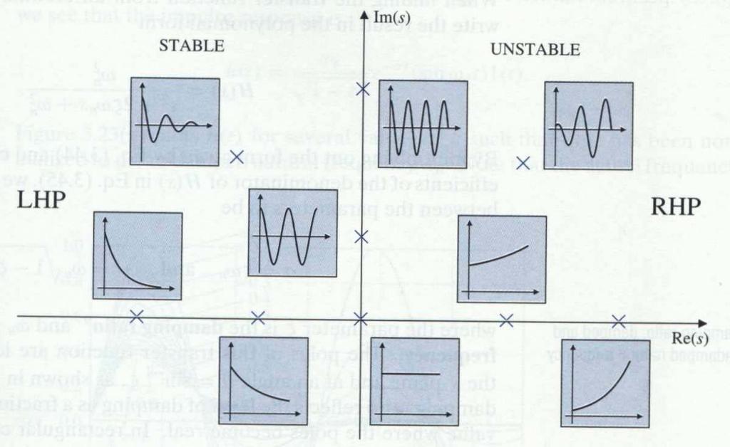
9 Stability Analysis from Closed Loop Transfer function Stable systems have closed-loop transfer functions with poles only in the left half-plane. Unstable systems have closed-loop transfer functions with at least one pole in the right half plane and/or poles of multiplicity greater than one on the imaginary axis. Marginally Stable systems have closed-loop transfer functions with only imaginary axis poles of multiplicity 1 and poles in the left half-plane. 9

10 Stability of closed loop system with gain variation As gain is increased from 3 to 7, the system becomes unstable 10

11 Routh Hurwitz Approach for Stability Analysis Dr. Radhakant Padhi Asst. Professor Dept. of Aerospace Engineering Indian Institute of Science - Bangalore

12 Sufficient Conditions for Instability and Marginal Stability: A system is Unstable if all signs of the coefficients of the denominator of the closed loop transfer function are not same. If powers of s are missing from the denominator of the closed loop transfer function, then the system is either Unstable or at best Marginally Stable Question: What if all coefficients are positive and no power of s is missing? Answer: Routh-Hurwitz criterion. 12

13 Routh Hurwitz Edward Routh, 1831 (Quebec) (Cambridge, England) Adolf Hurwitz, 1859 (Germany)-1919 (Zurich) 13

14 Routh Hurwitz Criterion Caution: This method tells how many closed loop system poles are in the left-half plane, in the righthalf plane and on the jω axis. However, it does not tell the location of the poles. Methodology o Construct a Routh table o Interpret the Routh table: The sign of the entries of the first column imbeds the information about the stability of the closed loop system. 14

15 Generating Routh Table from Closed loop Transfer Function Initial layout for Routh table: 15

16 Generating Routh Table : Completed Routh table Note: Any row of the Routh table can be multiplied by a positive constant 16

17 Interpreting the Routh Table The no. of roots of the polynomial that are in the right half-plane is equal to the number of sign changes in the first column. A system is Stable if there are no sign changes in the first column of the Routh table. 17

18 Example : Ref : N. S. Nise, Control Systems Engineering, 4 th Ed. Wiley,

19 Example : Solution: Since all the coefficients of the closed-loop characteristic 3 2 equation s + 10s + 31s are present, the system passes the Hurwitz test. So we must construct the Routh array in order to test the stability further. 19

20 Example : it is clear that column 1 of the Routh array is: it has two sign changes ( from 1 to -72 and from -72 to 103). Hence the system is unstable with two poles in the righthalf plane. 20

21 Routh-Hurwitz Criterion: Special Cases The basic Routh table check fails in the following two cases: Zero only in the first column of a row Entire row consisting of zeros These cases need further analysis 21

22 Special Case 1: Zero only in the first column (1) Replace zero by ε. Then let ε 0 either from left or right. ( d) (2) Replace s by 1/. The resulting ploynomial will have roots which are reciprocal of the roots of the original polynomial. Hence they will have the same sign. The resulting ploynomial can be written by a polynomial with coefficient in reverse order. 22

23 Special Case 2: Entire row that consists of zeros Form the Auxiliary equation from the row above the row of zero Differentiate the polynomial with respect to s and replace the row of zero by its Coefficients Continue with the construction of the Routh table and infer about the stability from the number of sign changes in the first column 23

24 Stabilizing control gain design via Routh-Hurwitz Objective: To find the range of gain K for the following system to be stable, unstable and marginally stable, assuming K > 0. Gs () H() s = 1 24

25 Stability analysis via Routh- Hurwitz criterion Closed loop transfer function: Cs () Gs () K T() s = = = 3 2 R() s 1 + G() s H() s s + 18s + 77s+ K Routh Table: 25

26 Stability design via Routh- Hurwitz : If If If K K K < 1386 system is stable (three poles in the LHS) > 1386 system is unstable (two poles in RHS one in LHS) = 1386 then an entire row will be zero. 2 Then the auxiliary equation is ( ) dp() s ds = 36s + 0 Routh table (with K = 1386) Ps = s + The system is Stable (marginally stable) 26

27 Steady State Error Analysis Dr. Radhakant Padhi Asst. Professor Dept. of Aerospace Engineering Indian Institute of Science - Bangalore

28 Definition and Test Inputs Steady-state error is the difference between the input and the output for a prescribed test input as t Usual test inputs used for steady-state error analysis and design are Step, Ramp and Parabola inputs (justification comes from the Taylor series analysis). 28

29 Test Inputs Test waveforms for evaluating steady-state errors of control systems 29

30 Evaluating Steady State Errors Ref: N. S. Nise, Control Systems Engineering, 4 th Ed. Wiley, Figure : Steady-state error: a. step input b. ramp input 30

31 Evaluating Steady State Errors a. General Representation b. Representation for unity feedback systems 31

32 Steady-State Error for Unity Feedback Systems Steady-State Error in Terms of T(s), Es () = Rs () Cs () Cs () = RsTs () () Es () = Rs ()[1 Ts ()] Applying Final Value Theorem, e( ) = lim e( t) = lim se( s) t s 0 s 0 e( ) = lim sr( s)[1 T( s)] 32

33 An Example Problem : Find the steady-state error for the system if T s = s + s+ 2 ( ) 5/( 7 10) and the input is a unit step. Solution : Rs = s Ts = s + s+ 2 () 1/ and () 5/( 7 10) = This yields Es ( ) ( s 7s 5) / ss ( 7s 10) since T( s) is stable, by final value theorem, e( ) = 1/ 2 33

34 Steady-State Error for Unity Feedback Systems.. Steady State Error in Terms of G(s) Es () = Rs () Cs () Cs () = EsGs () () ( ) Es () = Rs ()/1 + Gs () By Final ValueTheorem, e sr() s + Gs ( ) = lim s 0 1 ( ) Note: Input Rs ( ) and System Gs ( ) allow us to calculate steady-state error e( ) 34

35 Effect of input on steady-state error : Step Input : R() s = 1/ s e s(1/ s) 1 ( ) = estep ( ) = lim = s Gs ( ) 1 + lim Gs ( ) s 0 For zerosteady-stateerror, lim Gs ( ) =. Hence Gs If s 0 Gs ( ) must have the form: ( s+ z )( s+ z ) () = andn 1 n s ( s+ p1)( s+ p2)... n = 0, then the system will have finite steady state error. 35

36 Effect of input on steady-state error.. Ramp Input : Rs () = 1/ s 2 2 s(1/ s ) 1 1 e( ) = eramp ( ) = lim = lim = s 01 + Gs ( ) s 0 s+ sgs ( ) lim sgs ( ) For zero steady-state error, lim sg( s) =. Hence Gs s 0 Gs ( ) must have the form: ( s+ z )( s+ z ) () = andn 2 n s ( s+ p1)( s+ p2)... s 0 36

37 Effect of input on steady-state error.. Parabolic input : Rs () = 1/ s 3 3 s(1/ s ) 1 1 s 0 s s 0 2 e( ) = eparabola ( ) = lim = lim = 1 Gs ( ) s sgs ( ) lim sgs ( ) For zero steady-state error, lim sgs ( ) = s 0 Hence Gs ( ) must have the form: ( s+ z )( s+ z )... G s = 1 2 () and n 3 n s ( s+ p1)( s+ p2)... 37

38 An Example Objective : To find the steady-state errors of the following system 2 for inputs of 5 ut ( ), 5 tut ( )and 5 tut ( ), where ut ( ) is the unit step function. 38

39 Example Solution : First we verify that the closed loop system is stable. Next, carryout the following analysis. 2 2 The Laplace transform of 5 ( ), 5 ( ), 5 ( )are 5 /, 5 / and 5 / respectively e( = ) estep ( ) = = = 1 + limgs () s 0 s e( ) = eramp ( ) = = = lim sg( s) e( ) = eparabola ( ) = = =. sgs ut tut tut s s s lim 2 ( ) 0 s 0 39

40 Static Error Constants and System Type : The steady-stateerror performance specifications arecalled "static error constants", defined as follows: Position constant K = lim G( s) s 0 Velocity constant K = lim sg( s) Acceleration constant K p v a s 0 2 = lim sgs ( ) s 0 "System Type"is the value of n in the denominator of G( s); ie.. Number of pure integrators in the forward path. Note: n = 0,1,2 indicates Type 0,1,2 system respectively. 40

41 Relationship between input, system type, static error constants and steady state errors Ref: N.S.Nise, Control Systems Engineering,4 th Ed. Wiley,

42 Interpreting the steady-state error specification : Question : What information is contained in K = 1000? Answer : The system is stable. The system is Type 0, since K is finite. If the input signal is unit step, then e( ) = = = K p p p 42

43 Steady-State Error for Disturbance Inputs [ ] [ ] Es () = Rs () Cs () = Rs () EsG () sg() s + DsG () () s 1 + G ( s) G ( s) E( s) = R( s) D( s) G ( s) G () s Es Rs Ds E s E s 2 () = () () = R() + D() 1 + G1( s) G2( s) 1 + G1( s) G2( s) Hence the steady state error ( s) can be reduced by either increasing G ( s) or decreasing G ( s). E 1 2 D 43

44 Steady-State Error for Non-unity Feedback Systems Forming an Equivalent Unity Feedback System 44

45 Sensitivity The degree to which changes in system parameters affect system transfer functions, and hence performance, is called sensitivity. The greater the sensitivity, the less desirable the effect of a parameter change. 45

46 Sensitivity S FP : = = lim ΔP 0 Fractionalchangein the parameter lim ΔP 0 Fractional change in the function ΔF/ F ΔP/ P P ΔF P F = lim = ΔP 0 F ΔP F P F P Note : In some cases feedback reduces the sensitivity of a system's steady-state error to changes in system parameters. 46

47 Example Ramp input: R( s) = 1/ K e v = lim sg( s) = ramp s 0 1 = = K v a K K a s 2 S S ea : a e a 1 = = = 1 e a a/ K K K e K a = = = 1 e K a/ K K ek : 2 47

48 48

49 49