IFCS Tutorial, San Francisco, 1 May The Leeson effect. Phase noise and frequency stability in oscillators. Enrico Rubiola

Size: px

Start display at page:

Download "IFCS Tutorial, San Francisco, 1 May The Leeson effect. Phase noise and frequency stability in oscillators. Enrico Rubiola"

Vernon Malone
5 years ago
Views:

IFCS Tutorial, San Francisco, May 20 The Leeson effect Phase noise and frequency

Contents The Leeson effect in a nutshell Phase noise and friends (*) Heuristic

theory Formal proof for the Leeson effect the Leeson effect in delay-line oscillators

1 IFCS Tutorial, San Francisco, May 20 The Leeson effect Phase noise and frequency stability in oscillators Enrico Rubiola CNRS FEMTO-ST Institute, Besancon, France Contents The Leeson effect in a nutshell Phase noise and friends (*) Heuristic explanation of the Leeson effect Phase noise in amplifiers Oscillator hacking Resonator theory Formal proof for the Leeson effect the Leeson effect in delay-line oscillators AM-PM noise coupling Acknowledgement and conclusions home page (*) covered by other tutorials

2 2 The Leeson effect in a nutshell David B. Leeson, A simple model for feed back oscillator noise, Proc. IEEE 54(2):329 (Feb 966) resonator out % S! " f # $ & " ' #2 0 ( 2Q f 2 oscillator noise noise S ) " f # ampli noise oscillator noise S! " f # Leeson effect noise of electronic circuits f L =! 0 /2Q f

3 3 Notation ν --> carrier frequency f --> Fourier analysis ω either 2πν or 2πf τ either measurement time relaxation time

4 4 -- optional -- Phase noise & friends Notation ν --> carrier frequency f --> Fourier analysis ω either 2πν or 2πf

5 Physical concept of PSD 5 file: sp-prism-sa Continuous spectrum S n n 2 > n n target P white light prism red violet sensor array or photo film λ ν v(t) input -Hz filter array f rms voltmeter rms voltmeter Sv (f ) f 2 Sv (f 2 ) Sv(fn) S Discrete spectrum Parallel spectrum analyzer f n rms voltmeter Sv (f n ) f

6 Clock signal affected by noise 6 Time Domain Phasor Representation Figures are from E. Rubiola, Phase noise and frequency stability in oscillators, Cambridge University Press α(t) φ(t) V 0 V 0 v(t) v(t) amplitude fluctuation V 0 α(t) [volts] normalized ampl. fluct. α(t) [adimensional] phase fluctuation ϕ(t) [rad] phase time (fluct.) x(t) [seconds] t t V 0 / 2 ampl. fluct. (V 0 / 2)α(t) phase fluctuation ϕ(t) V 0 / 2 polar coordinates Cartesian coordinates v(t) = V 0 [ + α(t)] cos [ω 0 t + ϕ(t)] v(t) = V 0 cos ω 0 t + n c (t) cos ω 0 t n s (t) sin ω 0 t under low noise approximation n c (t) V 0 and n s (t) V 0 It holds that α(t) = n c(t) and ϕ(t) = n s(t) V 0 V 0

7 Physical quantities 7 v(t) = V 0 [ + α(t)] cos [2πν 0 t + ϕ(t)] Allow φ(t) to exceed ±π and count the number of turns, so that φ(t) describes the clock fluctuation in full phase noise radian ϕ(t) ( ν)(t) = 2π dϕ(t) dt Hertz ( ν)(t) frequency fluctuation x = ϕ 2πν 0 y(t) = 2πν 0 dϕ(t) dt y(t) = ν 0 ( ν)(t) phase-time (fluctuation) x(t) second y(t) = dx(t) dt y(t) dimensionless fractionalfrequency fluctuation

8 Phase noise & friends 8 v(t) =V p [ + α(t)] cos [2πν 0 t + ϕ(t)] S ϕ (f) random walk freq. b 4 f 4 signal sources only S ϕ (f) = PSD of ϕ(t) power spectral density L(f) = 2 S ϕ(f) dbc random fractional-frequency fluctuation y(t) = random phase fluctuation it is measured as S ϕ (f) = T E {Φ(f)Φ (f)} S ϕ (f) T Φ(f)Φ (f) m ϕ(t) S y = f 2 2πν 0 ν0 2 S ϕ (f) Allan variance (two-sample wavelet-like variance) 2 σy(τ) 2 = E y 2 k+ y k (expectation) (average) approaches a half-octave bandpass filter (for white noise), hence it converges even with processes steeper than /f. S y (f) σ y 2 (τ) random walk freq. flicker phase white phase h 2 f 2 h f white freq. h 0 /2τ flicker freq. b 3 f 3 h 0 flicker freq. white freq. white freq. x b 2 f 2 b f f 2 / ν2 0 h 2ln(2)h f flicker freq. flicker phase. h 2 f 2 flicker phase both signal sources and two-port devices white phase white phase freq. drift random walk freq. (2π) 2 h 6 2 τ b 0 f f τ Figures are from E. Rubiola, Phase noise and frequency stability in oscillators, Cambridge University Press

9 Skip Allan variance 9 definition σ 2 y(τ) =E { ] } 2 [y 2 k+ y k σ 2 y(τ) =E { [ 2 τ (k+2)τ (k+)τ y(t) dt τ (k+)τ kτ ] } 2 y(t) dt wavelet-like variance { [ + σy(τ) 2 =E ] } 2 y(t) w A (t) dt w A = 2τ 0 <t<τ 2τ τ<t<2τ 0 elsewhere w A 0 0 τ 2τ 2 τ 2 τ time t energy E{w A } = + w 2 A(t) dt = τ the Allan variance differs from a wavelet variance in the normalization on power, instead of on energy

10 0 Relationships between spectra and variances noise type S ϕ (f) S y (f) S ϕ S y σ 2 y(τ) mod σ 2 y(τ) white PM b 0 h 2 f 2 h 2 = b 0 ν 2 0 3f H h 2 (2π) 2 τ 2 2πτf H 3f H τ 0 h 2 (2π) 2 τ 3 flicker PM b f h f h = b ν 2 0 [ ln(2πf H τ)] h (2π) 2 τ h τ 2 n white FM flicker FM b 2 f 2 h 0 h 0 = b 2 ν 2 0 b 3 f 3 h f h = b 3 ν h 0 τ 4 h 0 τ 2 ln(2) h ln(2) h random walk FM b 4f 4 h 2 f 2 h 2 = b 4 ν 2 0 (2π) 2 h 2 τ (2π)2 6 h 2 τ linear frequency drift ẏ 2 (ẏ)2 τ 2 2 (ẏ)2 τ 2 f H is the high cutoff frequency, needed for the noise power to be finite.

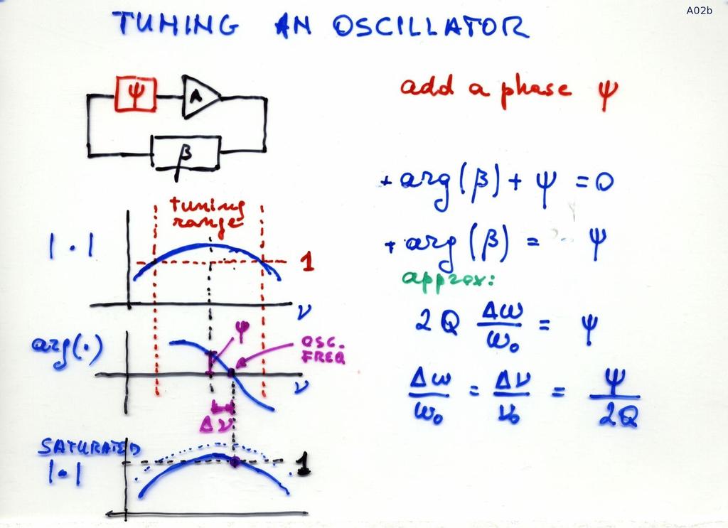
11 Heuristic explanation of the Leeson effect

12 2 General oscillator model real amplifier noise PM %(t) AM $(t) A [+!(t)] cos[" 0 t+#(t)] gain compression resonator! Barkhausen condition Aβ = at ω0 (phase matching) The model also describes the negative-r oscillator resonator negative-r amplifier! V sense compression AM-PM noise

13 3

14 4

5 Heuristic derivation of the Leeson formula fast fluctuation: no

ψ(t) ν0 ν = ψ static 2Q ν 2 0 S ν (f ) = Sψ (f ) 2Q ν0 2 Sϕ (f ) =

15 5 Heuristic derivation of the Leeson formula fast fluctuation: no feedback slow fluctuations: ψ Δν conversion φ Sϕ (f ) = Sψ (f ) fast or slow? Q τ= πν0 ν0 2 Sψ (f ) Sϕ (f ) = + 2 f 2Q Sϕ (f )/Sψ (f ) ϕ(t) = ψ(t) ν0 ν = ψ static 2Q ν 2 0 S ν (f ) = Sψ (f ) 2Q ν0 2 Sϕ (f ) = 2 Sψ (f ) integral f 2Q /f 2 ν0 fl = 2Q f0 f fl Though obtained with simplifications, this result turns out to be is exact

16 Oscillator noise 6 -- real sustaining amplifier -- Figures are from E. Rubiola, Phase noise and frequency stability in oscillators, Cambridge University Press S ϕ (f) b 3 f 3 x f 2 b f amplifier flicker freq f c x Type b 2 f 2 white freq f 2 f L f L > f c b 0 white phase f S ϕ (f) x f 2 b 3 f 3 flicker freq amplifier f L Type 2 b f flicker phase f c f L < f c b 0 white phase f The sustaining-amplifier noise is Sφ(f) = b0 + b /f (white and flicker)

17 The effect of the output buffer 7 Cascading two amplifiers, flicker noise adds as Sφ(f) = [Sφ(f)] + [Sφ(f)]2 S ϕ (f) output buffer /f 3 output buffer /f sustain. ampli. S ϕ (f) /f /f 3 sustain. ampli. f c intersection Type A total noise the output buffer noise is not visible /f 2 f L Type 2A /f f<f L f 0 f L > f c f 0 f L < f c total noise f 0 f f 0 S ϕ (f) output buffer S ϕ (f) lower /f 3 /f lower /f 3 /f sustain. ampli. output buffer f c /f 2 sustain. ampli. /f Type B /f f L intersection f L > f c total noise low flicker sustaining amplifier (noise corrected) and normal output buffer /f noise appears Type 2B total noise low flicker sustaining amplifier (noise corrected) and normal output buffer f<f L f 0 f 0 f 0 f f L < f c f 0 f L f c f Figures are from E. Rubiola, Phase noise and frequency stability in oscillators, Cambridge University Press f L f c f

18 The resonator natural frequency fluctuates 8 The oscillator tracks the resonator natural frequency, hence its fluctuations The fluctuations of the resonator natural frequency contain /f and /f 2 (frequency flicker and random walk), thus /f 3 and /f 4 of the oscillator phase The resonator bandwidth does not apply to the natural-frequency fluctuation. (Tip: an oscillator can be frequency modulated ar a rate >> fl) S ϕ (f) /f 3 buffer S ϕ (f) buffer /f /f 3 /f 4 sustain. ampli. /f 4 sustain. ampli. f L f c /f Type A electronics resonator /f 3 /f 3 /f 2 /f /f 2 /f f 0 f 0 f L Type 2A /f f c f L > f c f L < f c electronics resonator f 0 f 0 S ϕ (f) /f 3 /f 3 /f f f S ϕ (f) buffer buffer /f 3 /f 4 /f 4 /f sustain. ampli. Figures are from E. Rubiola, Phase noise and frequency stability in oscillators, Cambridge University Press f c f L /f 3 sustain. ampli. Type B Type 2B f c /f f L f L > f c electronics resonator f L < f c electronics resonator f 0 f 0 f 0 f f 0 f

19 Skip Phase noise > frequency stability 9 S ϕ (f) r. w. freq. b 4 f 4 phase noise b 3 f 3 flicker freq. white freq. b 2 f 2 flicker phase. b f white phase b 0 f frequency noise S y (f) h 2 f 2 x f 2 / ν2 0 h 2 f 2 r. w. freq. h f h 0 flicker freq. white freq. h f flicker phase white phase f Allan variance white! σ 2 (τ) = h0/2τ flicker! σ 2 (τ) = 2ln(2) h- r.walk! σ 2 (τ) = ((2π) 2 /6) h0τ σ y 2 (τ) flicker phase white phase white freq. flicker freq. r. w. freq. freq. drift τ

20 AM-PM noise in amplifiers 20

21 Amplifier white and flicker noise 2 S! (f), log-log scale b! const. vs. P 0 b f flicker thermal b 0 = FkT 0 / P 0 b 0, higher P 0 b 0, lower P 0 f' c f" c f f c = ( b / FkT 0 ) P 0 depends on P 0 Thermal noise kt0 = W/Hz ( 74 dbm/hz) Noise figure F photodetector b 20 dbrad 2 /Hz Rubiola & al. IEEE Trans. MTT (& JLT) 54 (2) p (2006) typical amplifier phase noise RATE GaAs HBT SiGe HBT Si bipolar microwave microwave HF/UHF fair good best unit dbrad 2 /Hz

22 The difference between additive 22 and parametric noise additive noise parametric noise u(t) input Σ z(t) noise-free amplifier RF noise, close to! 0 v(t) output u(t) input AM x(t) PM y(t) noise-free amplifier near-dc noise v(t) output PSD file: amp-add-vs-param Sz(f) (noise) stopband sum passband! 0 Sv(f) (output) Su(f) (input) stopband PSD Sy(f) (noise) up-conversion stopband passband! 0 Sv(f) (output) Su(f) (input)!! stopband the noise sidebands are independent of the carrier the noise sidebands are proportional to the carrier

a 2 + b 2 + c 2 + d 2 = Correlation between AM and PM noise 23 R. Boudot, E. Rubiola, arxiv:00.2047v, Jan 200. Also IEEE T MTT (submitted) u(t) input file: AM-PM-correl a a=b=0.

23 a 2 + b 2 + c 2 + d 2 = Correlation between AM and PM noise 23 R. Boudot, E. Rubiola, arxiv: v, Jan 200. Also IEEE T MTT (submitted) u(t) input file: AM-PM-correl a a=b=0.7 c=d=0 AM c x(t) b PM d y(t) noise-free amplifier correlated noise z(t) v(t) output a=0.4 b=0.4 c=0.2 d=0.8 The need for this model comes from the physics of popular amplifiers Bipolar transistor. The fluctuation of the carriers in the base region acts on the base thickness, thus on the gain, and on the capacitance of the reverse-biased basecollector junction. Field-effect transistor. The fluctuation of the carriers in the channel acts on the drain-source current, and also on the gatechannel capacitance because the distance between the `electrodes' is affected by the channel thickness. Laser amplifier. The fluctuation of the pump power acts on the density of the excited atoms, and in turn on gain, on maximum power, and on refraction index. a=0.4 b=0.92 c=d=0 a=b=0 c=d=0.7 AM and PM fluctuations are correlated because originate from the same near-dc random process

24 Amplitude-phase coupling in amplifiers 24!!%#!'##!'%#!&##!&%#!$## *+,-./ /45 6Ω7 *+,-./0 +4;953/45<6µA7!(?)!" # Real part!(?@!>!>?'!>?&!>?$!>?"!>?% % & 6$ # 7!>?(!$%# $!>?> /:,.+39;<6µ=7 $ # #!"## # &## "## (## )## '### '&## /:,.+39;<6µ=7!>?) # &## "## (## )## '### '&## Oscillation amplitude is hidden in the current Imaginary part In the gain-compression region, RF amplitude affects the phase The consequence is that AM noise turns into PM noise Well established fact in quartz oscillators (Colpitts and other schemes) Similar phenomenon occurs in other types of (sustaining) amplifier R. Brendel & E. Rubiola, Proc IFCS p , Geneva CH, 28 may - Jun 2007

25 Oscillator Hacking 25

26 The spectrum is Agilent. The figure is from E. Rubiola, Phase noise and frequency stability in oscillators, Cambridge University Press Analysis of commercial oscillators 26 The purpose of this section is to help to understand the oscillator inside from the phase noise spectra, plus some technical information. I have chosen some commercial oscillators as an example. The conclusions about each oscillator represent only my understanding based on experience and on the data sheets published on the manufacturer web site. You should be aware that this process of interpretation is not free from errors. My conclusions were not submitted to manufacturers before writing, for their comments could not be included. S!(f) dbrad 2 /Hz b coefficient b 3 coefficient /f 3 baseline oscillator /f Agilent prototype 0 MHz OCXO 40 ruler /f baseline set square Fourier frequency, Hz

27 The spectrum is Miteq. The figure is from E. Rubiola, Phase noise and frequency stability in oscillators, Cambridge University Press Miteq D20B, 0 GHz DRO S ϕ (f) dbrad 2 /Hz Phase noise of the 0 GHz DRO Miteq D20B b 3 = +37 dbrad 2 /Hz (b ) ampli = 98dBrad 2 /Hz dB difference Fourier frequency, Hz b 0 b 2 = dbrad 2 /Hz = 46dBrad 2 /Hz 6 Digitized spectrum 4dB difference 7 From the table σ 2 y = h0/2τ+2ln(2)h h0 = b 2/ν 2 0 h = b 3/ν 2 0 f c =70kHz f L =4.3MHz kt0 = W/Hz ( 74 dbm/hz) floor 46 dbrad 2 /Hz, guess F =.25 ( db) => P0 = 2 µw ( 27 dbm) fl = 4.3 MHz, fl = ν0/2q => Q = 60 fc = 70 khz, b /f = b0 => b = ( 98 dbrad 2 /Hz) [sust.ampli] h0 = and h = => σy = 2 0 / τ

28 The spectrum is Poseidon. The figure is from E. Rubiola, Phase noise and frequency stability in oscillators, Cambridge University Press Poseidon Scientific Instruments Shoebox 0 GHz sapphire whispering-gallery () Poseidon Shoebox 0 GHz sapphire WG resonator noise correction 0 phase noise, dbc/hz oscillator b 3 f 3 instrument background d ~ 6dB b f f L =2.6kHz Fourier frequency, Hz fl = v0/2q = 2.6 khz => Q = This incompatible with the resonator technology. Typical Q of a sapphire whispering gallery resonator: K (room temp), K (liquid N), 4 0 4K (liquid He). In addition, d ~ 6 db does not fit the power-law. The interpretation shown is wrong, and the Leeson frequency is somewhere else

29 The spectrum is Poseidon. The figure is from E. Rubiola, Phase noise and frequency stability in oscillators, Cambridge University Press The /f noise of the output buffer is higher than that of the sustaining amplifier (a complex amplifier with interferometric noise reduction / or a Pound control) In this case both /f and /f 2 are present white noise 69 dbrad 2 /Hz, guess F = 5 db (interferometer) => P0 = 0 dbm buffer flicker 20 dbrad 2 Hz => good microwave amplifier fl = v0/2q = 25 khz => Q = (quite reasonable) fc = 850 Hz => flicker of the interferometric amplifier 39 dbrad 2 Hz 29 Poseidon Scientific Instruments Shoebox 0 GHz sapphire whispering-gallery (2) Poseidon Shoebox 0 GHz sapphire WG resonator noise correction phase noise, dbc/hz oscillator f to f 3 conversion f c =850Hz (b ) ampli = 40 dbrad 2 /Hz instr. background f 0 to f 2 conversion (b ) buffer = 20dBrad 2 /Hz (b 0 ) ampli = 69 dbrad 2 /Hz f L =25kHz Fourier frequency, Hz

30 The spectrum is Poseidon. The figure is from E. Rubiola, Phase noise and frequency stability in oscillators, Cambridge University Press Poseidon Scientific Instruments 30 0 GHz dielectric resonator oscillator (DRO) SSB phase noise, dbc/hz dB/dec b dbrad 2 3 =+4 /Hz DRO 0.4 XPL slope 25 db/dec DRO 0.4 FR b = 65dBrad 2 /Hz Phase noise of two PSI DRO 0.4 FR f c =9.3kHz 7dB b 0 = 65dBrad 2 /Hz slope close to 25dB/dec 0 5 Fourier frequency, Hz 20dB/dec 3dB difference f L =3.2MHz floor 65 dbrad 2 /Hz, guess F =.25 ( db) => P0 = 60 µw ( 8 dbm) fl = 3.2 MHz, fl = ν0/2q => Q = 625 fc = 9.3 khz, b /f = b0 => b = ( 25 dbrad 2 /Hz) [sust.ampli, too low] Slopes are not in agreement with the theory

31 The spectrum is Oscolloquartz. The figure is from E. Rubiola, Phase noise and frequency stability in oscillators, Cambridge University Press Example Oscilloquartz 8600 (wrong) E. Rubiola Phase noise and frequency stability in oscillators Cambridge University Press 2008 ISBN b 3 = 24dBrad 2 /Hz b = 3dBrad 2/Hz Oscilloquartz OCXO MHz OCXO Courtesy of Oscilloquartz SA, comments of E. Rubiola b 0 = 55dBrad 2/Hz 87 File: 603 osa 8600 mod st f L = 2.2Hz Fourier frequency, Hz f = 250Hz c ANALYSIS floor S!0 = 55 dbrad2/hz, guess F = db! P0 = 8 dbm 2 ampli flicker S! = 32 dbrad 2 Hz! good RF amplifier 3 merit factor Q = " 0 /2f L = 5 06/5 = 06 (seems too low) 4 take away some flicker for the output buffer: * flicker in the oscillator core is lower than 32 Hz * f L is higher than 2.5 Hz * the resonator Q is lower than 0 6 This is inconsistent with the resonator technology (expect Q > 06). The true Leeson frequency is lower than the frequency labeled as f L The /f 3 noise is attributed to the fluctuation of the quartz resonant frequency

32 The spectrum is Oscilloquartz. The figure is from E. Rubiola, Phase noise and frequency stability in oscillators, Cambridge University Press Example Oscilloquartz 8600 (right) 32 S ϕ (f) dbrad 2 /Hz E. Rubiola Phase noise and frequency stability in oscillators Cambridge University Press 2008 ISBN resonator instability b 3 = 24dBrad 2 /Hz Leeson effect (hidden) sust. ampli + buffer b = 3dBrad 2/Hz Oscilloquartz OCXO MHz OCXO Courtesy of Oscilloquartz SA, comments of E. Rubiola b 0 = 55dBrad 2/Hz 67 File: 604 osa 8600 mod Fourier frequency, Hz f =.4Hz L (guessed) f = 4.5Hz L f = 63Hz c sustaining amplifier b 2 = 37dBrad /Hz F=dB b0 => P0= 8 dbm (b 3)osc => σy=.5x0 3, Q=5.6x0 5 (too low) Q.8x0 6 => σy=4.6x0 4 Leeson (too low)

33 The spectrum is IEEE. The figure is from E. Rubiola, Phase noise and frequency stability in oscillators, Cambridge University Press Skip Whispering gallery oscillator, liquid-n2 temp 33 dbrad 2 /Hz S ϕ (f) Prototype of 9 GHz whispering gallery oscillator (liquid N, 77 K) 77 Woode & al, IEEE TUFFC 43(5), a: free running b 3 = 50 dbrad 2 /Hz b: electronics 97 c: system floor 07 b = 0dBrad 2 /Hz 7 b dbrad 2 0 = 36 /Hz b 3 = 77 dbrad 2 /Hz Fourier frequency, Hz a b c f L = 360Hz f c = 3.kHz

34 The spectrum is Oscilloquartz. The figure is from E. Rubiola, Phase noise and frequency stability in oscillators, Cambridge University Press Skip Example Oscilloquartz S ϕ (f) dbrad 2 /Hz E. Rubiola Phase noise and frequency stability in oscillators Cambridge University Press 2008 ISBN Oscilloquartz OCXO MHz OCXO Courtesy of Oscilloquartz SA, comments of E. Rubiola (b dbrad 2 3 ) tot = 28.5 /Hz f L=.6Hz fl=.25hz <= Q=2x0 6? f" L=3.2Hz (b => ) tot Q=7.9x0 5 = 32.5dBrad 2 /Hz b 0 = 53dBrad 2 /Hz 67 File: 605 osa 8607 mod 0 (b ) osc = 38.5dBrad 2 /Hz Fourier frequency, Hz F=dB b0 => P0= 20 dbm (b 3)osc => σy=8.8x0 4, Q=7.8x0 5 (too low) Q 2x0 6 => σy=3.5x0 4 Leeson (too low)

35 The spectrum is Poseidon. The figure is from E. Rubiola, Phase noise and frequency stability in oscillators, Cambridge University Press Skip Example CMAC Pharao 35 S ϕ (f) dbrad 2 /Hz E. Rubiola Phase noise and frequency stability in oscillators Cambridge University Press 2008 ISBN (b 3 ) tot = 32 dbrad 2 /Hz Rakon Pharao 5 MHz OCXO Courtesy of Rakon, comments of E. Rubiola f L=.5Hz f" L=3Hz f =50Hz c technology Q=2x0 6? 60 => f L =.25Hz 70 0 File: 606 candelier bw 0 fc =3Hz 2 (b ) tot (b )osc b 0 = 35.5 Fourier frequency, Hz = 52.5 dbrad 2 /Hz dbrad 2 /Hz = 4.5 dbrad 2 /Hz F=dB b0 => P0= 20.5 dbm (b 3)osc => σy=5.9x0 4, Q=8.4x0 5 (too low) Q 2x0 6 => σy=2.5x0 4 Leeson (too low)

36 The spectrum is Rakon. The figure is from E. Rubiola, Phase noise and frequency stability in oscillators, Cambridge University Press Skip Example FEMTO-ST prototype 36 S ϕ (f) dbrad 2 /Hz resonator instability = 6.6 dbrad 2 /Hz b 3 Leeson effect (hidden) dbrad 2 FEMTO ST prototype b 3 = 23.2 /Hz LD cut, 0 MHz, Q =.5x0 6 sustaining = 36 amplifier b dbrad 2 /Hz sust. ampli + buffer b dbrad 2 = 30 /Hz apparent 3dB b = 47 dbrad 2 0 /Hz 3dB File: 607 femtost mod E. Rubiola Phase noise and frequency stability in oscillators Cambridge University Press 2008 ISBN f L =4.3Hz calculated f =9.3Hz L apparent Fourier frequency, Hz F=dB b0 => P0= 26 dbm (b 3)osc => σy=.7x0 3, Q=5.4x0 5 (too low) (there is a problem) Q=.5x0 6 => σy=8.x0 4 Leeson (too low)

37 The spectrum is Agilent. The figure is from E. Rubiola, Phase noise and frequency stability in oscillators, Cambridge University Press Skip Example Agilent dbrad Sϕ (f) /Hz Measurement System Rolloff b 3 = 03 db /f 3 sust. ampli + buf b = 3 db E. Rubiola Phase noise and frequency stability in oscillators Cambridge University Press 2008 ISBN sust. amplifier b = 37 db Agilent 08 0 MHz OCXO Courtesy of Agilent Technologies Comments of E. Rubiola experimental data /f b 0 = 62 db /f 0 Noise Floor 67 File: bw 0 ~ 7Hz (guess!) f L f L =50Hz f c 0 =320Hz frequency, Hz F=dB b0 => P0= dbm (b 3)osc => σy=8.3x0 3, Q=x0 5 (too low) Q 7x0 5 => σy=.2x0 3 Leeson (too low)

38 The spectrum is IEEE. The figure is from E. Rubiola, Phase noise and frequency stability in oscillators, Cambridge University Press Skip Example Agilent prototype 38 ϕ (f) 80 dbrad S File: 609 karlq xtal /Hz b 3= 02 dbrad 2 /Hz sust. ampli + buf b = 26 dbrad 2 /Hz simple sust. amplifier b = 32 dbrad 2 /Hz b 0 Agilent prototype 0 MHz OCXO Courtesy of the IEEE Comments of E. Rubiola = 58 dbrad 2 /Hz 60 upper bound 80 0 f c =4Hz f L possible ~ 7Hz E. Rubiola Phase noise and frequency stability in oscillators Cambridge University Press 2008 ISBN Fourier frequency, Hz f L =320Hz corrected sust. amplifier (guess!) b = 52 dbrad 2 /Hz F=dB b0 => P0= 2 dbm (b 3)osc => σy=9.3x0 3 Q=.6x0 5 Q 7x0 5 => σy=2.x0 3 (Leeson)

39 Skip Interpretation of Sφ(f) [] 39 Only quartz-crystal oscillators real phase-noise spectrum Figures are from E. Rubiola, Phase noise and frequency stability in oscillators, Cambridge University Press E. Rubiola Phase noise and frequency stability in oscillators Cambridge University Press 2008 ISBN start from b f take away the buffer /f noise estimatef L evaluate ν Q 0 s = 2f L File: 602a xtal interpretation S ϕ (f) after parametric estimation b 3 f 3 sustaining ampli b a f Leeson effect? f L f L f c flicker b f buffer + sust.ampli b 0 f 0 f ~ 6dB Sanity check: power P0 at amplifier input Allan deviation σy (floor) 2 3 buffer stages => the sustaining amplifier contributes 25% of the total /f noise

40 Skip Interpretation of Sφ(f) [2] 40 Only quartz-crystal oscillators E. Rubiola Phase noise and frequency stability in oscillators Cambridge University Press 2008 ISBN Figures are from E. Rubiola, Phase noise and frequency stability in oscillators, Cambridge University Press technology => Q t f L ν 0 = 2Qt the Leeson effect is hidden S ϕ (f) x f 2 b 3 f 3 resonator /f freq. noise sustaining ampli File: 602b xtal interpretation f L f L f L f c f Technology suggests a quality factor Qt. In all xtal oscillators we find Qt Qs

41 Skip Example Wenzel Figures are from E. Rubiola, Phase noise and frequency stability in oscillators, Cambridge University Press S ϕ (f) dbrad 2 /Hz ampli noise (?) 30dB/dec b 3 = 67dBrad 2 /Hz b 0 = 73 dbrad 2 /Hz E. Rubiola Phase noise and frequency stability in oscillators Cambridge University Press 2008 ISBN Leeson effect (hidden) is about here Wenzel MHz OCXO Comments of E. Rubiola specifications Data are from the manufacturer web site. Interpretation and mistakes are of the authors. Estimating (b )ampli is difficult because there is no visible /f region 80 0 File: 60 mywenzel f L =3.5kHz guess Q=8x0 4 => f L =625Hz Fourier frequency, Hz F=dB b0 => P0=0 dbm (b 3)osc => σy=5.3x0 2 Q=.4x0 4 Q 8x0 4 => σy=9.3x0 3 (Leeson)

42 The Table is from E. Rubiola, Phase noise and frequency stability in oscillators, Cambridge University Press Quartz-oscillator summary 42 Oscillator ν 0 (b 3 ) tot (b ) tot (b ) amp f L f L Q s Q t f L (b 3 ) L R Note Oscilloquartz () Oscilloquartz () Rakon Pharao (2) FEMTO-ST LD prot (3) Agilent (4) Agilent prototype (5) Wenzel ? 38? (6) unit MHz db rad 2 /Hz db rad 2 /Hz db rad 2 /Hz Hz Hz (none) (none) Hz db rad 2 /Hz Notes () Data are from specifications, full options about low noise and high stability. (2) Measured by Rakon on a sample. Rakon confirmed that <Q< in actual conditions. (3) LD cut, built and measured in our laboratory, yet by a different team. Q t is known. (4) Measured by Hewlett Packard (now Agilent) on a sample. (5) Implements a bridge scheme for the degeneration of the amplifier noise. Same resonator of the Agilent 08. (6) Data are from specifications. db R = (σ y) oscill (σ y ) Leeson = floor (b 3 ) tot (b 3 ) L = Q t Q s = f L f L

43 Opto-electronic oscillator 43 Courtesy of OEwaves (handwritten notes are mine). Cut from the oscillator specifications available at the URL

44 The spectrum is OEwaves. The figure is from E. Rubiola, Phase noise and frequency stability in oscillators, Cambridge University Press Skip Opto-electronic oscillator 44 OEwaves Tidalwave photonic oscillator (0 GHz) b 4 = + dbrad 2 /Hz (+8 dbc/hz) ~ f L 7kHz? (wild guess) b = 2 b 3 dbrad2 /Hz 0 ~ ( 24 dbc/hz) b 2 =?? 38 dbrad 2 /Hz ( 4 dbc/hz) Courtesy of OEwaves (handwritten notes are mine). Cut from the oscillator specifications available at the URL

45 Skip Opto-electronic oscillator 45 b 8 = +2 dbrad 2 /Hz (??) OEwaves OEO, the lowest phase noise (2007) b 3 = 50 dbrad 2 /Hz min = 56 dbrad 2 /Hz b 2 = 8 dbrad 2 /Hz Courtesy of OEwaves, notes are mine

The spectrum is IEEE. The figure is from E. Rubiola, Phase noise and frequency stability in oscillators, Cambridge University Press Skip Opto-electronic oscillator 46 NIST 0.

46 The spectrum is IEEE. The figure is from E. Rubiola, Phase noise and frequency stability in oscillators, Cambridge University Press Skip Opto-electronic oscillator 46 NIST 0.6 GHz OEO, Römisch & al, IEEE UFFC 27(5) p.59 (2000) Phase noise, dbrad 2 /Hz b 4 = +2 dbrad2 /Hz b 3 = 0 dbrad 2 /Hz b 2 = 42 dbrad 2 /Hz min = 37 dbrad 2 /Hz Fourier frequency, Hz

47 The spectrum is IEEE. The figure is from E. Rubiola, Phase noise and frequency stability in oscillators, Cambridge University Press Skip Opto-electronic oscillator (amplifier) 47 OEO amplifier, Römisch & al, IEEE UFFC 27(5) p.59 (2000) Phase noise, dbrad 2 /Hz b = 09 dbrad 2 /Hz b 0 = 39 dbrad 2 /Hz

48 Skip Opto-electronic oscillator simulation 48 Figures are from E. Rubiola, Phase noise and frequency stability in oscillators, Cambridge University Press e 05 e 06 e 07 e 08 e 09 e 0 e e 2 e 3 phase noise Sphi(f) S.Romisch delay line oscillator oscillator amplifier parameters: tau = 5.9E 6 s m = nu_m = 0.6 GHz Q = 8300 b_0 = 3 db b_ = 98 db file le calc romisch src allplots leeson e 4 frequency, Hz e e+05 e+06

49 Things may not be that simple 49 +,-./023./ :; %" #" " )#" )%" )'" )*" )!"" )!#" Merrer & al - (OEO) - Proc IFCS 2009, Fig.8 )!%"!"!!" #!" $!" %!" &!" '!" ( b 3 = σ y = B/=0456C; <=/>?/7@ 49:; " )#" )%" This could be due to AM/PM coupling )'" )*" )!""!"A!*('!"A!*(*!"A!**"!"A!**#!"A!**% <=/>?/7@04D9:; Savchenkov & al, Opt. Lett 35(0) , 5 may 200, Fig.2 & 0 db/dec 5 db/dec File: 959-rin-em4rin Source: oeo-spectra Original: EM4RIN.pdf K. Volyanskiy, 2008 E.Rubiola, April 200 Maleki & al, Recent advances in OE signal generation, IEEE conf Phased Array 2000 p36 Fig. experiment /f 3 theory fractionary slopes b 0 =4 0 4 /f 2 background 35 db/dec 30 db/dec 25 db/dec 20 db/dec o4 Frequency from carrier (Hz)

50 Resonator theory 50

51 Resonator time domain 5 Figures are from E. Rubiola, Phase noise and frequency stability in oscillators, Cambridge University Press ẍ + ω n Q ẋ + ω2 nx = ω n Q v(t) i(t) shorthand: f = ω/2π v(t) Z L inductor = sl d v L (t) = L i(t) dt Z R =R resistor v R (t) = R i(t) ω n Q τ ω p i(t) natural frequency quality factor relaxation time τ = 2Q ω n free-decay pseudofrequency ω p = ω n /4Q 2 envelope e t/τ t Z C = sc capacitor v C (t) = t i(t ) dt C 0 relaxation time τ = 2Q ω n /f p ω n f p = 2π 4Q 2

52 Resonator frequency domain 52 β(s) = ω n Q s ω n s 2 + s +ω Q n 2 s = σ + jω Figures are from E. Rubiola, Phase noise and frequency stability in oscillators, Cambridge University Press β(jω) lin lin plot argβ(jω) +π/2 frequency domain ω n ω n Q / 2 ( 3dB) +π/4 ω s=oo σ p + jω p σ p = complex plane ω n 2Q jω ω n ω p = = ω n 2Q 4Q 2 ω n 4Q 2 σ lin lin plot π/2 π/4 ω σ p jω p

53 53 χ = ω ω n ω n ω β = {β} = {β} = β 2 = +jqχ +Q 2 χ 2 Qχ +Q 2 χ 2 +Q 2 χ 2 arg(β) = arctan(qχ)

54 Linear time-invariant (LTI) systems 54 time domain δ(t) LTI system h(t) impulse response Figures are from E. Rubiola, Phase noise and frequency stability in oscillators, Cambridge University Press Fourier transform Laplace transform v i (t) LTI system v i (t) * h(t) ejωt H(jω) ejωt LTI system V i (j ω) H(jω) V LTI i (j ω) system e st V i (s) LTI system LTI system H(s) e st H(s) V i (s) response to the generic signal vi(t) H(ω) = H(s) = h(t) e jωt dt h(t) e st dt 0 H(s), s=σ+jω, is the analytic continuation of H(ω) for causal system, where h(t)=0 for t<0 Noise spectra Si ( ω) LTI system H(jω) 2 Si ( ω)

55 Laplace-transform patterns 55 Fundamental theorem of complex algebra: F(s) is completely determined by its roots F (s) = s +/τ F (s) = s s 2 +2s/τ + ω 2 n Figures are from E. Rubiola, Phase noise and frequency stability in oscillators, Cambridge University Press complex plane 0 5 x complex plane j * omega sigma x j * omega sigma.0 exp( t/tau) tangent t/tau time t/tau exp( t/tau) 2 time t/tau complex plane 40 j * omega x x o 40 complex plane 40 j * omega x 20 sigma o x sigma cos(omega*t) * exp( t/tau) envelope exp( t/tau) envelope tangent t/tau time t/tau cos(omega*t) * exp( t/tau) envelope exp( t/tau) time t/tau complex plane 0 5 j * omega 20 5 exp( t/tau) tangent t/tau complex plane j * omega x 20 0 cos(omega*t) * exp( t/tau) envelope exp( t/tau) envelope tangent t/tau x sigma time t/tau file le calc laplace 2nd src allplots leeson o x sigma time t/tau

56 Resonator impulse response 56 &(t) &(t) [+"(t)] cos[! 0 t+#(t)] resonator Q,! n [+$(t)] cos[! 0 t+%(t)] 2nd order differential equation b $ (t) b % (t) Can t figure out a δ(t) of phase or amplitude? Use Heaviside (step) u(t) and differentiate set a small phase or amplitude step! at t=0, and linearize for!(0 cos(! 0 t) t = 0 resonator Q,! n cos[! 0 t+%(t)] [+$(t)]cos(! 0 t) relaxation time τ = 2Q exp(!t/tau) tangent!t/tau ω n b(t) = τ e t/τ B(s) = /τ s +/τ file: ele-resonator-delta-response cos(! 0 t+') or (+ ')cos(! 0 t) '!b(t) dt 0.2 time t/tau

57 Response to a phase step κ 57 A phase step is equivalent to switching a sinusoid off at t = 0, and switching a shifted sinusoid on at t=0 Figures are from E. Rubiola, Phase noise and frequency stability in oscillators, Cambridge University Press switched off at t = 0 switched on at t = 0 v I (t) v O (t) envelope v(t) phase 0 exponential decay cos(ω p t) e t/τ t v I (t) v O (t) phase κ v(t) exponential growth cos(ω p t + κ) e t/τ t envelope τ t τ t

58 Resonator impulse response (ω0=ωn) 58 v i (t) = cos(ω 0 t) u( t) switched off at t =0 + cos(ω 0 t + κ) u(t) switched on at t =0 phase step κ at t=0 v o (t) = cos(ω p t) e t/τ + cos(ω p t + κ) e t/τ t>0 v o (t) = cos(ω p t) κ sin(ω p t) e t/τ κ 0 output linearize v o (t) = cos(ω 0 t) κ sin(ω 0 t) e t/τ ω p ω 0 V o (t) = t/τ +jκ e 2 {Vo (t)} arctan κ e t/τ phasor angle {V o (t)} impulse response b(t) = τ e sτ B(s) = /τ high Q slow-varying phase vector delete κ and differentiate s +/τ

59 Detuned resonator (ω0 ωn) 59 amplitude phase α ϕ = bαα b ϕα b αϕ b ϕϕ ε ψ A Φ = Bαα B ϕα B αϕ B ϕϕ E Ψ Ω = ω 0 ω n β 0 = β(jω 0 ) θ = arg(β(jω 0 )) detuning mudulus phase v i (t) = β 0 cos(ω 0 t θ) u( t) switched off at t =0 + β 0 cos(ω 0 t θ + κ) u(t) switched on at t =0 phase step κ at t=0 = β 0 cos(ω 0 t θ) u( t)+ β 0 cos(ω0 t θ) cos κ sin(ω 0 t θ) sin κ u(t) β 0 cos(ω 0 t θ) u( t)+ β 0 cos(ω0 t θ) κ sin(ω 0 t θ) u(t) κ.

60 Skip Detuned resonator (cont.) 60 v o (t) = cos(ω 0 t) κ sin(ω 0 t)+κ sin(ω n t) e t/τ slow-varying phase vector output, large Q (ωp=ωn) use Ω = v o (t) = cos(ω 0 t) κ sin(ωt)e t/τ κ sin(ω 0 t) ω0 ωn cos(ωt)e t/τ V o (t) = 2 κ sin(ωt)e t/τ + jκ cos(ωt)e t/τ κ arctan {V o(t)} {V o (t)} = κ cos(ωt)e t/τ V o (t) = V o (0) κ sin(ωt)e t/τ angle amplitude b ϕϕ (t) = b αϕ (t) = impulse response Ω sin(ωt)+ τ cos(ωt) delete κ and differentiate e t/τ Ω cos(ωt)+ τ sin(ωt) e t/τ phase amplitude

61 check on the sign of b2 Skip Resonator step and impulse response 6 $"# $"!!"#!"!!!"# 5@+25F5@+25D,,+29F+29 ()*+,-*.+/0.*,/,)2*,3*)40*3,-*./05)/ *)*-8,3*)4090:,-*;4*0<=,>! >GHF% >GH >GH >GHF%! +29F5@+25D,,5@+25F+29 $"!!"#!"!!!"#!!?HI?HI?HIG%?HIG% ()*+,-./0.-*2-./3/45./ / ,*57G7,*57E//*5:G*5: *5:G7,*57E//7,*57G*5: 8707).4.09/6.4+2:2;/30.<+.2=>/? 9:4-*8,,?'#!-*./0!.)*+!-*.+/0.*./4-<*8,/.<9@@!57!0/9.* A",B4C9/@5D,E40,%!!? )97*D,)F)54!$"!!"!!"# $"! $"# %"! %"# &"! &"# '"!!$"! 3:;+0.9//@'A!0.-2!:)*+,-.!0.-* =.9/-=:,,!7)!2:-. B"/C+D:,7E/F+2/%!!@ 4:).E/4G47+!"!!"# $"! $"# %"! %"# &"! &"# '"! Ω sin Ωt + b (t) = τ cos Ωt e t/τ Ω cos Ωt + τ sin Ωt e t/τ Ω cos Ωt + τ sin Ωt e t/τ Ω sin Ωt + τ cos Ωt e t/τ

62 Skip 62

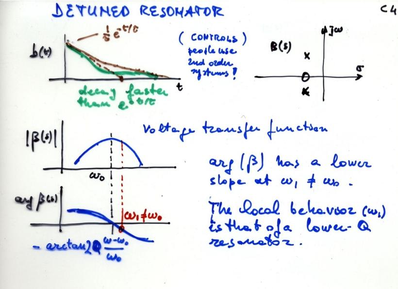
63 Skip Frequency response 63 A resonator tuned at resonator tuned at ω 0 ω L B(s) ω 0 j ω = ω n σ resonator detuned byω<<ω 0 +Ω Ω B resonator detuned ω L ω L (+Ω 2 τ 2 ) B(s) j ω σ phase noise transfer function B(jf) ^ F = Omega / (2pi) F = 0 F = f_l F = 0.5 f_l F =.5 f_l F = 2 f_l file le calc bigb src allplots leeson Figures are from E. Rubiola, Phase noise and frequency stability in oscillators, Cambridge University Press B (s) = diagonal terms τ normalized frequency f / f_l diagonal terms s + τ + Ω2 τ Ωs s τ s + τ + Ω 2 s τ s + τ + Ω 2 2 Ωs s + τ + Ω2 τ s τ s + τ + Ω 2 τ s τ s + τ + Ω 2 2 check on the sign of B2

64 Skip Frequency response 64 Roots & complex plane Frequency response off-diagonal terms off-diagonal terms B (s) = τ s + τ + Ω2 τ Ωs s τ s + τ + Ω 2 s τ s + τ + Ω 2 2 Ωs s + τ + Ω2 τ s τ s + τ + Ω 2 τ s τ s + τ + Ω 2 2 check on the sign of B2

65 65 Formal proof for the Leeson effect

66 E. Rubiola & R. Brendel, arxiv: v, [physics.ins-det] 66 Low-pass representation of AM-PM noise real amplifier noise PM %(t) AM $(t) A [+!(t)] cos[" 0 t+#(t)] gain compression RF, μwaves or optics resonator! low-pass equivalent PM AM & u (t) A u (s)!(t) "(s)! #(t) $(s) %(t)! u A v & v (t) A v (s) low-pass b(t) B(s) Leeson Effect The amplifier copies the input phase to the out adds phase noise gain fluctuat. '(t) N(s) low-pass b(t) B(s) extension of the LE to AM noise The amplifier compresses the amplitude adds amplitude noise saturation A u

67 Effect of feedback 67 Figures are from E. Rubiola, Phase noise and frequency stability in oscillators, Cambridge University Press A Oscillator transfer function H(s) j ω constant zeros Oscillator transfer function (RF) poles function of A increasing A B Detail of the denominator of H(s) A = 2Q A=0 open loop j ω A= oscillation A = +2Q negative feedback insufficient gain excessive gain σ negative feedback insufficient gain excessive gain σ A=0 A=

68 Leeson effect 68!(t) "(s) noisy amplifier! low-pass b(t) resonator A = #(t) $(s) B(s) = /τ s +/τ phase-noise transfer function H(s) = Φ(s) Ψ(s) H(s) = +AB(s) H(s) = +sτ sτ definition general feedback theory Leeson effect!(t) "(s) file: ele-pm-scheme v 2! low-pass relaxation time " = 2Q/# 0 #(t) $(s) v complex plane H(s) /τ j"! transfer function H(jf) 2 /f 2 f L f L = ν 0 2Q f 0 f

69 Oscillator with detuned resonator A B 69 resonator tuned at ω 0 H(s) j ω resonator detuned by Ω<<ω n H(s) j ω ω L Figures are from E. Rubiola, Phase noise and frequency stability in oscillators, Cambridge University Press phase noise transfer function H(jf) ^ F = 0 F =.5 f_l F = f_l F = 0.5 f_l F = 2 f_l σ +Ω Ω ω L file le calc bigh src allplots leeson F = Omega / (2pi) σ normalized frequency f / f_l

70 Low-pass model of amplitude () 70 First we need to relate the system restoring time τr to the relaxation time τ!(t) file: ele-am-scheme v 2! low-pass A v relaxation time " = 2Q/# 0 u = +" u v = +" v simple feedback theory u = + v 2 v 2 = (v v 2 ) dt τ v 2 = u v = v = Au u = + (A )u + dt τ differential equation u τ (A ) u = τ + Gain compression is necessary for the oscillation amplitude to be stable The Laplace / Heaviside formalism cannot be used because the amplifier is non-linear

71 Common types of gain saturation 7 A A 0 hard clipping A 0 soft clipping u A v A 0 van der Pol (quadratic) oscillator operation linear A=!(u-) file: ele-clipping-types u Gain compression is necessary for the oscillation amplitude to be stable

72 Low-pass model of amplitude (2) 72 Gain compression A 0 A =!(u ) homogeneous differential equation u τ (A ) u =0 u Three asymptotic cases At low RF amplitude, let the gain be an arbitrary value denoted with A0 A 0 Case A u Startup: u 0, A A0 > u τ (A 0 ) u =0 u = C e (A 0 ) t/τ rising exponential For small fluctuation of the stationary RF amplitude, the gain varies linearly with V Case B A =!(u ) u Regime: u, A = γ (u ) u + γ τ (u ) u =0 u = C γ t/τ 2e restoring time constant τr = τ/γ Simplification: the gain varies linearly with V in all the input range Case C A =!(u ) u Linear gain: A = γ (u ) u = u(0) e γt/τ +

73 Startup analysis vs. simulation 73 exponential saturation analytical solution, A = γ(u ) 0 MHz oscillator L = mh R = 25 Ω Q ~ 503 van der Pol oscillator simulated by RB Rising exponential. We find the same time constant τ/γ

74 Gain fluctuations definition 74 A fluctuating A=!(u-)+" oscillator operation fluctuation " ideal A=!(u-) u A v file: ele-gain-fluctuation u Gain compression is necessary for the oscillation amplitude to be stable

75 Gain fluctuations output is u 75!(t)! A u = +" u v = +" v u = τ (A )u non-linear equation A = γ(u ) + η file: ele-am-scheme v 2 low-pass v η relaxation time " = 2Q/# 0 u + γ τ (u )u = η τ u α u α u α u + γ τ α u = τ η linearization for low noise linearized equation Linearize for low noise and use the Laplace transforms α u (t) A u (s) and η(t) N (s) H u (s) = A u(s) N (s) definition s + γ τ H u (s) A u (s) = τ N (s) j" H u (jf) 2 /γ 2 Laplace transform H u (s) = /τ s + γ/τ result γ/τ! file: ele-hu-am γf L /f 2 f

76 Gain fluctuations output is v 76!(t) v 2! low-pass A v u = +" u η v = +" v s + γ τ s + γ τ A u (s) = τ N (s) A u (s) = A v(s) N (s) γ A v (s) = s + N (s) τ starting equation file: ele-am-scheme relaxation time " = 2Q/# 0 boring algebra relates αv to αu v = Au A = γ(u ) + + η H(s) = A v(s) N (s) H(s) = s +/τ s + γ/τ definition result v =[ γ(u ) + + η] u v =[ γα u ++η] [ + α u ] +α v =+η γα u + α u α u η γαu 2 α linearization v = ( γ)α u + η for low noise α u = α v η γ!< /# [!>] $/# /# $/# j" j"!! H(jf) 2 file: ele-h-am!<!> γf L Leeson f L γf L

77 Additive noise output is u 77!(t)! A u = +" u v = +" v u = τ (A )u + + τ A = γ(u ) non-linear equation file: ele-am-scheme v 2 low-pass v relaxation time " = 2Q/# 0 u + γ τ (u )u = + τ α u α u α u + γ τ α u = + τ lineariz. for low noise linearized equation Linearize for low noise and use the Laplace transforms α u (t) A u (s) and (t) E(s) H u (s) = A u(s) E(s) H u (s) = s +/τ s + γ/τ definition result s + γ τ!< /# [!>] $/# /# A u (s) = $/# j" j"!! s + τ H(jf) 2 file: ele-h-am!<!> E(s) γf L Leeson f L Laplace transform γf L

78 Additive noise output is v 78!(t) file: ele-am-scheme v 2! low-pass A v relaxation time " = 2Q/# 0 u = +" u boring algebra relates α to α v = Au A = γ(u ) v = [ γ(u )] u +α v = [ γα u ] [ + α u ] +α v =+α u γα u γαu 2 α v = ( γ)α u α u = α v γ v = +" v linearization for low noise γ α u + γ τ α u = + τ γ α u = α v /( γ) α v + γ τ α v = + τ s + γ τ H(s) = A v(s) E(s) A v (s) = s + τ H(s) = ( γ) s +/τ s + γ/τ!< /# [!>] $/# /# $/# j" j"!! H(jf) 2 file: ele-h-am!<!> γf L E(s) f L linearized equation Laplace transform definition Leeson result γf L

79 Parametric noise & AM-PM noise coupling 79 #(t) N(s) u = +" u " u (t) A u (s)! A u (s) A AM loop v = +" v " v (t) A v (s) Amplifier noise w # B "" H u (s) = /τ s + γ/τ H v (s) = s +/τ s + γ/τ x(t) (s) w! w! AM " PM coupling!"(t) $"(s)!'(t) $'(s)! &(s) B %% PM loop %(t) &(s) H ϕ (s) = +sτ sτ file: ele-am-pm-cpl-param-oeo E. Rubiola & R. Brendel, arxiv: v [physics.ins-det]

80 80 Effect of AM-PM noise coupling u A v A loop AM response h(t) t H(f)!f L f L f amplifier noise near-dc random process amplitude fluct "/! ideal A=!(u -) fluctuating A =!(u )+" +"/! u phase fluct. #' gain fluct. " loop AM response h(t) H(f) t fluctuating!f L f L f #' #" # = #'+#'' arg(a) ideal file: ele-am-pm-cpl-amp +"/! u Leeson effect E. Rubiola & R. Brendel, arxiv: v [physics.ins-det]

81 Noise transfer function, and spectra 8 AM-PM coupling shows up here!#$"&!#$"%!""""!""" '((#)*+,(+-. /.+),02345 /6768#*#79 *60+:+!;%<# &+++=>?+:+!;"#% :+";"% @(>?+:+%;"#A ),02345+:+ ";B E26)JC+?##9,4+#((#)* E20#C+-.+4,39# 7#KC+),8E34#K!#$"&!#$"%!""""!""" '((#)*+,(+-. /.+),02345 /6768#*#79 *60+:+!;%<# &+++=>?+:+!;"#% :+";"% @(>?+:+%;"#A ),02345+:+";B F26)KC+?##9,4+#((#)* F20#C+-.+4,39# 7#LC+),8F34#L!""!""!" (3507#C++<%& -. /. )2 9,07)#C+,9) ,39# ';+D0E3,26F+67+G"!"! (7#H0#4)I!""!"""!""""!#$"%!#$"&!" (3507#C++<%D -. /. )2 9,07)#C+,9) ,39# ';+E0F3,26G+67+H"!"! (7#I0#4)J!""!"""!""""!#$"%!#$"& Notice that the AM-PM coupling can increase or decrease the PM noise In a real oscillator, flicker noise shows up below some 0 khz In the flicker region, all plots are multiplied by /f

82 82 Leeson effect in the delay-line oscillator

83 83 Motivations optics tunable bandpass filter laser EOM β d β f PM AM A out delay line mode selector ψ(t) η(t) [+α(t)] cos[ω 0 t+φ(t)] Corning Potential for very-low phase noise in the 00 Hz MHz range Invented at JPL, X. S. Yao & L. Maleki, JOSAB 3(8) , Aug 996 Early attempt of noise modeling, S. Römisch & al., IEEE T UFFC 47(5) 59 65, Sep 2000 PM-noise analysis, E. Rubiola, Phase noise and frequency stability in oscillators, Cambridge 2008 [Chapter 5] Since, no progress in the analysis of noise at system level Nobody reported on the consequences of AM noise

84 E. Rubiola & R. Brendel, arxiv: v, [physics.ins-det] 84 Low-pass representation of AM-PM noise real amplifier noise PM ψ(t) AM η(t) A [+α(t)] cos[ω 0 t+φ(t)] gain compression μwave mode selector β f delay line β d low-pass equivalent PM AM α u (t) A u (s) ψ(t) Ψ(s) Σ φ(t) Φ(s) ε(t) Σ u A v α v (t) A v (s) low-pass & delay b(t) B(s) Leeson Effect The amplifier copies the input phase to the out adds phase noise gain fluctuat. η(t) N(s) low-pass & delay b(t) B(s) extension of the LE to AM noise The amplifier compresses the amplitude adds amplitude noise saturation A u

85 85 Leeson effect A = phase-noise transfer function ψ(t) Ψ(s) noisy amplifier Σ low-pass & delay b(t) B(s) feedback φ(t) Φ(s) B(s) = H(s) = Φ(s) Ψ(s) H(s) = e sτ H(s) = +sτ f +AB(s) +sτ f +sτ f e sτ definition general feedback theory Leeson effect H, complex plane transfer function H 2 This figure is from E. Rubiola, Phase noise and frequency stability in oscillators, Cambridge University Press! m 2Q! m = (2&/$ d ) m j! %! = # 2Q $ d %! = # 2Q $ d µ m µ m (2&/$ d ) µ (2&/$ d ) µ E. Rubiola, Phase noise and frequency stability in oscillators, Cambridge 2008

86 Gain fluctuations definition 86 A fluctuating A=!(u-)+" oscillator operation fluctuation " ideal A=!(u-) u A v file: ele-gain-fluctuation u Gain compression is necessary for the oscillation amplitude to be stable E. Rubiola & R. Brendel, arxiv: v [physics.ins-det]

Gain fluctuations output is u(t) 87 ε(t) E(s) file: ele-oeo-am-scheme Σ low-pass η Linearize for low noise and use the Laplace transform α u (t) A u (s) and η(t) N (s) A delay u =+α u α u (t) A u (s)

87 Gain fluctuations output is u(t) 87 ε(t) E(s) file: ele-oeo-am-scheme Σ low-pass η Linearize for low noise and use the Laplace transform α u (t) A u (s) and η(t) N (s) A delay u =+α u α u (t) A u (s) The low-pass has only 2nd order effect on AM H(s) = A u(s) N (s) τ definition v =+α v α v (t) A v (s) u = A(t τ) u(t τ) A = γ(u ) + η use u=α+, expand and linearize for low noise α(t) =( γ)α(t τ) γα 2 (t τ) + η(t τ)+η(t τ)α(t τ) non-linear equation linearized equation α(t) =( γ)α(t τ)+η(t τ) Laplace transform A u (s) = ( γ)e sτ = N (s) 0 0 H(s) = result ( γ)e sτ

88 Gain fluctuations output is v(t) 88 ε(t) E(s) file: ele-oeo-am-scheme Σ low-pass A delay boring algebra relates αv to αu v = Au A = γ(u ) + + η v =[ γ(u ) + + η] u η v =[ γα u ++η] [ + α u ] u =+α u α u (t) A u (s) The low-pass has only 2nd order effect on AM τ v =+α v α v (t) A v (s) use u=α+ A u (s) ( γ)e ıωτ = N (s) A u (s) = A v(s) N (s) γ H(s) = A v(s) N (s) starting equation + ( γ) e sτ A v (s) = ( γ)e sτ N (s) definition H(s) = + ( γ)( e sτ ) ( γ)e sτ result +α v =+η γα u + α u α u η γαu 2 α linearization v = ( γ)α u + η for low noise α u = α v η γ

89 Figures are IEEE Skip AM & PM spectra were anticipated 89 AM noise PSD, db/hz PM noise PSD, dbrad 2 /Hz selector roll-off Prediction is based on the stochastic diffusion (Langevin) theory However complex, the Langevin theory provides an independent check Y.K. Chembo & al., IEEE J. Quant. Electron. 45(2) p.78-86, Feb 2009

90 Parametric noise & AM-PM noise coupling 90 #(t) N(s) u = +" u " u (t) A u (s)! A u (s) A B "" AM loop v = +" v " v (t) A v (s) H v (s) = + ( γ) ( e sτ ) ( γ)e sτ Amplifier noise w # H u (s) = ( γ)e sτ x(t) (s) w! AM " PM coupling w!!"(t) $"(s)!'(t) $'(s)! &(s) B %% PM loop %(t) &(s) H ϕ (s) = +sτ f +sτ f e sτ file: ele-am-pm-cpl-param E. Rubiola & R. Brendel, arxiv: v [physics.ins-det]

91 Similar to the oscillator based on a simple resonator Effect of AM-PM noise coupling 9 u A v A loop AM response H(f) amplifier noise near-dc random process γf L f L f phase fluct. ψ' gain fluct. η amplitude fluct η/γ +η/γ ideal A= γ(u -) fluctuating A = γ(u )+η u fluctuating loop AM response H(f) ψ' ψ" γf L f L f ψ = ψ'+ψ'' arg(a) ideal file: ele-am-pm-cpl-amp-oeo +η/γ u Leeson effect E. Rubiola & R. Brendel, arxiv: v [physics.ins-det]

Similar to the oscillator based on a simple resonator Noise transfer function and spectra 92 AM-PM coupling shows up here Notice that the AM-PM coupling

92 Similar to the oscillator based on a simple resonator Noise transfer function and spectra 92 AM-PM coupling shows up here Notice that the AM-PM coupling can increase or decrease the PM noise In a real oscillator, flicker noise shows up below some 0 khz In the flicker region, all plots are multiplied by /f

93 The figure is OSA, comments are mine Noise spectra 93 Savchenkov & al, Opt. Lett 35(0) , 5 may 200, Fig.2 experiment AM-PM coupling? theory background A. Savchenkov & al, Opt. Lett 35(0) , 5 may 200, Fig.2

94 Noise spectra db/dec AM-PM coupling? 2 db lag OEO phase noise File: 949-SMF-ZD Source: 949-OEO-spectra Plot: SMF_ZD_bis E.Rubiola (K.V.) Sep 2009 S ψ [dbrad 2 /Hz] Leeson effect: f f f f f 2.5 SMF28 [ f 2.5 ] f L = 5.9 khz 40 Zero dispersion fiber Fig Frequency [Hz] Unfortunately, the awareness of this model come after the end of the experiments Spectrum from K. Volyanskiy & al., IEEE JLT (Submitted, Apr. 200)

95 The figures is NASA, comments are mine Noise spectra 95 AM-PM coupling? SSB PHASE NOISE, dbc/hz!40!60!80!00!20!40 SLC OSCILLATOR FREE RUNNING Yao & al - (Dual-loop OEO) Nasa TMO Report , Fig.6 HP 867B OEO ,000 FREQUENCY OFFSET, Hz X.S.Yao & al., NASA TMO Report (998), Fig. 6

96 Conclusions 96

97 Phase noise and frequency stability in oscillators Cambridge University Press, November 2008 ISBN 978-0-52-88677-2 hardback ISBN 978-0-52-5328-7 paperback Contents Forewords (L. Maleki, D. B.

97 97 Phase noise and frequency stability in oscillators Cambridge University Press, November 2008 ISBN hardback ISBN paperback Contents Forewords (L. Maleki, D. B. Leeson) Phase noise and frequency stability Phase noise in semiconductors & amplifiers Heuristic approach to the Leson effect Phase noise and feedback theory Noise in delay-line oscillators and lasers Oscillator hacking Appendix

98 E. Rubiola Experimental methods in AM-PM noise metrology book project 98 Roberto Bergonzo Front cover: The Wind Machines Artist view of the AM and PM noise Courtesy of Roberto Bergonzo,

99 Acknowledgements 99 I am grateful to Lute Maleki and to John Dick for numerous discussions during my visits at the NASA JPL, which are the first seed of my approach to the oscillator noise I am indebted to a number of colleagues and friends for invitations and stimulating discussions - dr. Tim Berenc, ANL, Argonne - dr. Holger Schlarb, DESY, Hambourg - prof. Theodor W. Hänsch and dr. Thomas Udem, MPQ-QO, München This material would never have existed without continuous discussions, help and support of Vincent Giordano, FEMTO-ST, over about 5 years This presentation is based on E.Rubiola, Phase noise and frequency stability in oscillators, Cambridge 2008, and on the complementary material E. Rubiola, R. Brendel, A generalization of the Leeson effect, arxiv: [physics.ins-det] Please visit my home page

100 Summary of relevant points 00 The Leeson effect consists in a phase-to-frequency conversion fully explained as a phase (noise) integration takes place below fl = ν0/2q The step response provides analytical solutions and physical inside. (Same formalism introduced by O. Heaviside in network theory) Buffer noise and resonator instability add to the Leeson effect Amplifier phase noise white noise: Sφ scales down as the carrier power P0 flicker noise: Sφ is independent of P0 Numerous oscillator spectra can be interpreted successfully The amplitude-noise response is similar to phase noise, but gain compression provides stabilization at low frequencies The theory indicates that amplitude-phase coupling results in a deviation from the polynomial law Unified AM/PM noise that applies to resonator-oscillators and to delay-line oscillators, including optical oscillators A bunch of free material is available on the author s home page

101 0 David and Enrico at the end of the tutorial Photo by Barbara Leeson, David s wife

On the 1/f noise in ultra-stable quartz oscillators

On the 1/f noise in ultra-stable quartz oscillators On the 1/ noise in ultra-stable quartz oscillators Enrico Rubiola and Vincent Giordano FEMTO-ST Institute, Besançon, France (CNRS and Université de Franche Comté) Outline Ampliier noise Leeson eect Interpretation