HW6. 1. Book problems 8.5, 8.6, 8.9, 8.23, 8.31

Transcription

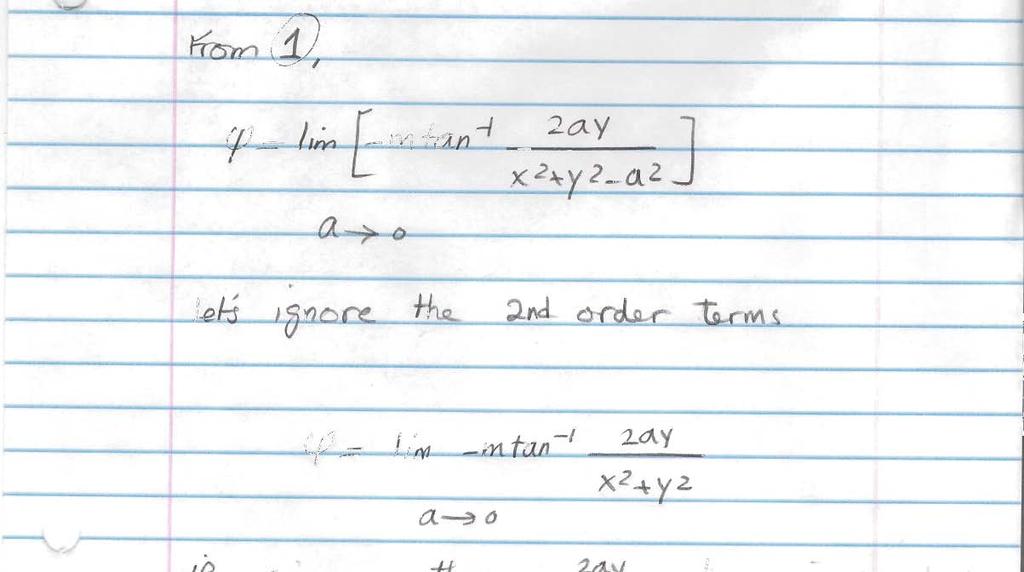
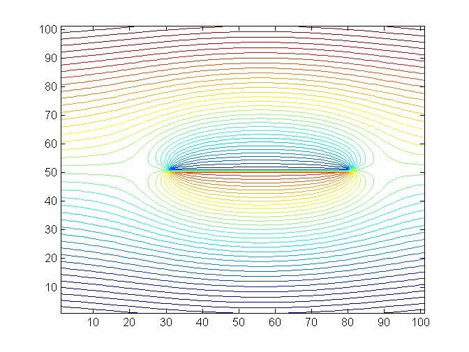
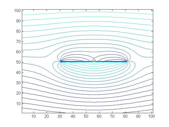
1 HW6 1. Book problems 8.5, 8.6, 8.9, 8.3, Add an equal strength sink and a source separated by a small distance, dx, and take the limit of dx approaching zero to obtain the following equations for a doublet λsinθ ψ =, r λcosθ φ = r 3. Use the given MATLAB code (posted on the web) and evaluate the following flow fields a. A sink at point (0.1, 0) with strength of -3 plus a source at point (-0.1, 0) with strength 3 b. Rankine Half Body: A source at point (-0., 0) with strength of plus a uniform flow of strength 0 m/s c. Rankine Oval: A source at point (-0., 0) with strength of, a sink at point (0.3, 0) with strength of, a uniform flow of strength 0 m/s. d. Add a vortex of strength 1 located at point (0.05, 0) to part c. 4. For a cylindrical surface surrounding the flow field in part (d) of problem 3 calculate the force on this surface if the surface is located at r=50.

2 Chapter 8 Potential Flow and Computational Fluid Dynamics 563 Solution: Evaluation of the laplacian of (1/r) shows that it is not legitimate: = = = r r 0 Illegitimate Ans. 3 r r r r r r r r r 8.5 Consider the two-dimensional velocity distribution u = By, v = +Bx, where B is a constant. If this flow possesses a stream function, find its form. If it has a velocity potential, find that also. Compute the local angular velocity of the flow, if any, and describe what the flow might represent. Solution: It does has a stream function, because it satisfies continuity: u v + = = 0 (OK); Thus u = By = ψ and v = Bx = ψ x y y x B Solve for ψ = ( x + y ) + const Ans. It does not have a velocity potential, because it has a non-zero curl: v u ω = curl V = k = = φ k[b ( B)] Bk 0 thus does not exist Ans. x y The flow represents solid-body rotation at uniform clockwise angular velocity B. 8.6 If the velocity potential of a realistic two-dimensional flow is φ = Cln(x + y ) 1/, where C is a constant, find the form of the stream function ψ ( x, y). Hint: Try polar coordinates. Solution: Using polar coordinates is certainly an excellent hint! Then the velocity potential translates simply to φ = C ln(r), which is a line source. Equation (8.1b) also shows that, Eq. (8.1 ): 1 y b ψ = Cθ = Ctan Ans x. 8.7 Consider a flow with constant density and viscosity. If the flow possesses a velocity potential as defined by Eq. (8.1), show that it exactly satisfies the full Navier-Stokes equation (4.38). If this is so, why do we back away from the full Navier-Stokes equation in solving potential flows?

3 564 Solutions Manual Fluid Mechanics, Fifth Edition Solution: If V = φ, the full Navier-Stokes equation is satisfied identically: dv ρ = p + ρ g+ µ V dt becomes φ V ρ + = p ( ρ gz) + µ ( φ), where the last term is zero. t The viscous (final) term drops out identically for potential flow, and what remains is φ V p gz = constant ( Bernoulli s equation ) t ρ The Bernoulli relation is an exact solution of Navier-Stokes for potential flow. We don t exactly back away, we need also to solve φ = 0 in order to find the velocity potential. 8.8 For the velocity distribution of Prob. 8.5, u = By, v = +Bx, evaluate the circulation Γ around the rectangular closed curve defined by (x, y) = (1, 1), (3, 1), (3, ), and (1, ). Solution: Given Γ = V ds around the curve, divide the rectangle into (a, b, c, d) pieces as shown: Fig. P8.8 Γ= u ds + v ds + u ds + v ds = ( B)() + (3B)(1) + (B)() + ( B)(1) a b c d or Γ=+4B Ans. Since, from Prob. 8.5, curl V = B, also Γ = curl V A region = (B)() = 4B. (Check) 8.9 Consider the two-dimensional flow u = Ax, v = +Ay, where A is a constant. Evaluate the circulation Γ around the rectangular closed curve defined by (x, y) = (1, 1), (4, 1), (4, 3), and (1, 3). Interpret your result especially vis-a-vis the velocity potential. Fig. P8.9

4 57 Solutions Manual Fluid Mechanics, Fifth Edition Solution: This pattern is the same as Fig. 8.6 in the text, except it is upside down. There is a stagnation point at (x, y) = (0, K/U). Ans. Fig. P Find the resultant velocity vector induced at point A in Fig. P8.3 due to the combination of uniform stream, vortex, and line source. Solution: The velocities caused by each term stream, vortex, and sink are shown at right. They have to be added together vectorially to give the final result: Fig. P8.3 m V = 11.3 at θ = 44. Ans. s 8.4 Line sources of equal strength m = Ua, where U is a reference velocity, are placed at (x, y) = (0, a) and (0, a). Sketch the stream and potential lines in the upper half plane. Is y = 0 a wall? If so, sketch the pressure coefficient p p C p = along the wall, where p 0 is the pressure at (0, 0). Find the minimum pressure point and indicate 1 ρu 0

5 Chapter 8 Potential Flow and Computational Fluid Dynamics A Rankine half-body is formed as shown in Fig. P8.31. For the conditions shown, compute (a) the source strength m in m /s; (b) the distance a; (c) the distance h; and (d) the total velocity at point A. Solution: The vertical distance above the origin is a known multiple of m and a: Fig. P8.31 πm πm πa yx= 0= 3 m = = =, U (7) m or m 13.4 and a 1.91 m Ans. (a, b) s The distance h is found from the equation for the body streamline: m( π θ) 13.4( π θ) 4.0 At x = 4 m, r body = = =, solve for θ 47.8 Usinθ 7sinθ cosθ Then r = 4.0/cos(47.8 ) = 5.95 m and h= r sin θ 4.41 m Ans. (c) A The resultant velocity at point A is then computed from Eq. (8.18): 1/ a a m VA= U 1+ + cosθa = cos Ans. (d) r r s 1/ 8.3 Sketch the streamlines, especially the body shape, due to equal line sources m at ( a, 0) and (+a, 0) plus a uniform stream U = ma. y C m m L x Fig. P8.3 Solution: As shown, a half-body shape is formed quite similar to the Rankine half-body. The stagnation point, for this special case U = ma, is at x = ( 1 )a =.41a. The halfbody shape would vary with the dimensionless source-strength parameter (U a/m).

6

7

8

9

10

11

12

13

14

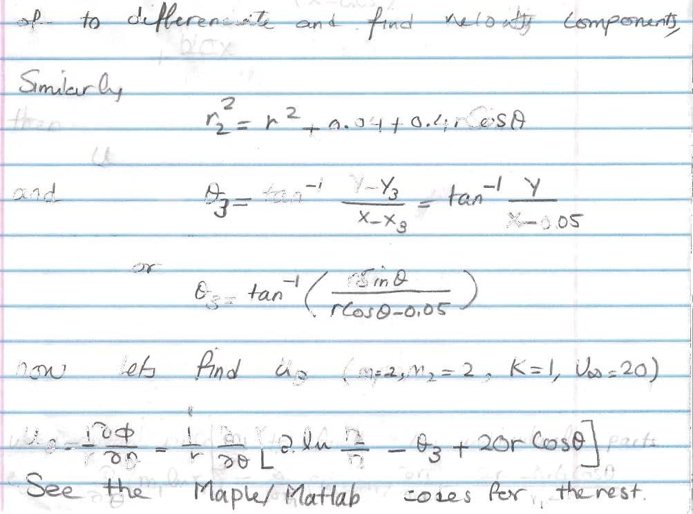
15 m1 := K m := K := 1 Uinf := 0 r1 := r C 0.09 K 0.6 r cos(q) r := q3 := arctan0 r C 0.04 C 0.4 r cos(q) r sin(q) r cos(q) K f := Kln(r C 0.09 K 0.6 r cos(q))cln(r C 0.04 r sin(q) C 0.4 r cos(q))karctan0 C 0 r cos(q) r cos(q) K vt := r sin(q) r K r C 0.09 K 0.6 r cos(q) K 0.4 r sin(q) r C 0.04 C 0.4 r cos(q) K r cos(q) r cos(q) K 0.05 C r sin(q) (r cos(q) K 0.05) r sin(q) K 0 r sin(q) 1 C (r cos(q) K 0.05)

16 r K 0.6 cos(q) vr := K r C 0.09 K 0.6 r cos(q) r C 0.4 cos(q) C r C 0.04 C 0.4 r cos(q) K sin(q) r cos(q) K 0.05 K r sin(q) cos(q) (r cos(q) K 0.05) 1 C r sin(q) (r cos(q) K 0.05) C 0 cos(q) r := 50. V = p = ρ Drag = Lift = V ( V V ) r π 0 + V π 0 θ pcosθ psinθ ( r.b.dθ) ( r.b.dθ) Drag := K b r Lift := K b r