Chapter 3-Elastic Scattering Small-Angle, Elastic Scattering from Atoms Head-On Elastic Collision in 1-D

Transcription

1 1 Chapter 3-Elastic Scattering Small-Angle, Elastic Scattering from Atoms To understand the basics mechanisms for the scattering of high-energy electrons off of stationary atoms, it is sufficient to picture an atom as a spherical cloud of electrons bound to a point-like nucleus. For an element with atomic number Z, the nucleus has Z protons and a net charge of + Ze. For a neutral atom, the electron cloud has Z electrons and a net charge of Ze. Because these electrons are rapidly orbiting the nucleus, we can treat them, for now, as a charge distribution, and ignore their discrete nature. The charge density drops off rapidly at radial distances outside the highest-energy, valence electron orbitals. The electrostatic potential of a bare, ionic nucleus would have a 1 r dependence on radius. But for a neutral atom, the electron cloud screens the nuclear charge at large radius. Gauss s Law says that, at a radius r from the nucleus, the potential only includes the net charge inside a spherical shell around the atom at the same radius. In other words, the electrons outside this shell do not contribute to the potential seen by an incident electron. The minimum distance between the line describing initial trajectory of an incident high-energy electron and the nucleus of an isolated atom is called the impact parameter b. For large values of b, the electron will slightly penetrate the electron cloud, with a slight reduction of the electron screening of the nucleus, causing a small deflection towards the nucleus (because opposite charges attract) as the electron scatters in the forward direction. For small b, the incident electron penetrates well into the electron cloud, and is deflected more substantially; it might even be backscattered. Transmission only involves forward scattering, so the signal in TEM primarily results from this large b, grazing-incidence electrons that don t substantially penetrate the electron cloud. We will see that this is mostly elastic scattering at low angles, and that these forward-scattered electrons are mostly coherent with respect to the incident beam. Most TEM imaging and diffraction data is generated by these small-angle, elastically-scattered electrons. Head-On Elastic Collision in 1-D For the moment, let s assume our incident electron is perfectly on target ( b = ) towards the nucleus of an isolated, stationary atom, somehow floating freely in space. Initially, the electron carries all of the energy and momentum. We know the atom has a much larger mass ( M ) than the electron (mass m ). Energy is conserved in elastic collisions; momentum is conserved in all collisions.

2 The initial and final kinetic energy are equal: E = E + E 1f f Conservation of momentum requires that the center-of-mass speed stay constant, too: v COM m ( ) = v m+ M Combining these, we have two possible outcomes. These can be distinguished by the final speed of the particle 1: v, forward v1 f = vcom ± ( v vcom ) = M m ( ) v, back M + m 1) Forward scattering: The electron continues in the forward direction ( = ) with the same kinetic energy and velocity that it had initially. The atom does not budge. (Somehow, the electron passed right through the atom.) Since the electron energy has not changed, its wavelength has not changed. Assuming there are no random phase shifts involved, this scattered electron wave is coherent with respect to the incident wave. ) Back scattering: The electron bounces backward ( = 18 ) towards the direction it came from. But to conserve momentum, the atom must continue, though very slowly, in the forward direction. Apparently, the electron transferred some kinetic energy to the atom, so the electron speed must have been slightly reduced by the collision. Even though the scattering is elastic, the scattered electron wave is not coherent with respect to the incident wave. Grazing-Incidence Elastic Collision Forward Scattering With slightly more effort, we can analyze the more general case of elastic scattering at grazing incidence (relatively large b) of an electron off a stationary atom. The electron will continue in the forward direction with only a slight deflection from its initial path. To conserve momentum, the atom must also move with a small transverse velocity, and it will necessarily have some small forward velocity, too. But, as in the head-on case, the large mass of the atom ensures that almost no kinetic energy is transferred to the atom in the collision. Therefore, the electron energy is essentially unchanged, only its direction of motion of changed, so the scattered wave is coherent with respect to the incident wave.

3 3 Nearly Head-On Elastic Collision Backscattering The same analysis used above reveals that a backscattered electron is expected to transfer some of its kinetic energy to the target atom. Thus, even if the collisionis elastic,, the electron loses energy in the process, and the scattered wave is incoherent with respect to the incident wave. Plane Waves: Sinusoidal Form A plane wave has a single direction of propagation. If the wavelength is λ, the particle momentum is p= h λ. But momentum is a vector, so we can write p= hk, where k is called the wave vector and points in the propagation direction. The length of k, k = 1 wave travels at the phase velocity λ, is sometimes called the wavenumber. The v p. We can use either a sine or cosine functions to describe the wave. Once we know the amplitude A and phase φ, the wave is defined at every point in space ( r ) and time (t). For example: ψ ( r, t) = A cos[ πk ( r t v p ) +φ] The are many alternative forms. For example, the frequency can be used: ψ ( r, t) = A cos[ π( k r f t) +φ] Plane Waves: Complex Exponential Form On a fundamental level, complex exponentials provide more appropriate descriptions of waves, compared i to the sinusoidal functions to which they are related by the Euler relation: e = cos+ isin. For one thing, complex exponentials allow the amplitude and phase to be combined into a single, complex number, for example ψ = A e iφ, giving the form π (, t) e i kr ft ψ r =ψ ( ) For an incident plane wave, we often normalize ( A = 1), and pick a phase of zero ( φ= ), so ψ = 1, giving.

4 4 π (, t) e i kr ft ψ r = ( ) Operators We need to take a look at what the wave function (for a plane wave) above tell us about particles, particularly electrons. The wave function contains all the available information about the electron s motion. Its momentum is found by applying the momentum operator p ˆ = i : i ψ ( r) = ( hk) ψ( r) We have again used the gradient operator = xˆ + yˆ + zˆ x y z Notice that ˆp acting on ψ( r ) returns the momentum hk times ψ( r ). So the wave function for a plane wave is an eigenfunction of the momentum operator, meaning that it is a state of well-defined momentum. Conversely, this wave function specified that the position of the electron is completely unknown, as you may expect from Heisenberg s Uncertainty Principle. What about energy? The energy of the particle is E = hf, which the energy operator Ê i = tells us: t i ψ ( r, t) = E ψ ( r, t) t It is not surprising that the plane wave is also an eigenfunction of energy. For a free particle, if we know its momentum, we know its energy. Schrodinger equation Let s consider a free, non-relativistic particle. Its energy is all kinetic: E = p m. The operator form of this is called the Hamiltonian: Here ˆ pˆ H = = m m is the Laplacian: x y z = + + We know the wave function for our plane wave: π (, t) e i kr ft ψ r =ψ ( ) We saw that this is an eigenfunction of the energy operator, meaning that it has a well-defined energy. So it is also an eigenfunction of the Hamiltonian, with the same eigenvalue: H ˆ ψ ( r, t) = Eψ( r, t) Combining this with the result from the previous section:

5 5 ˆ Hψ ( r, t) = i ψ( r, t) t This is the Schrodinger equation. It applies to the wave function of any non-relativistic particle, not just a free electron. If the particle is in a potential, we have to include that energy term in the Hamiltonian: pˆ Hˆ = + U r = + U m m r ( ) ( ) In essence, the SE relates the time and space aspects of the wave function. Energy eigenstates We saw that the plane wave was an energy eigenstate. Its wave function is separable into space and time functions. ( kr ) ψ ( r, t) =ψ e =ψ( r) e πi f t ie t When we evaluate the SE, the time factors can be canceled: [ ] H ˆ ψ( r) e ie t E ( ) e ie = ψ r t So, again: Ĥψ ( r) = E ψ( r ) The time-independent part of the wave function satisfies this time-independent SE. Since the wave function describes an energy eigenstate, the space part of the wave function contains all of the energy information. In this case, there is no reason to keep writing the time factor, so we have reduced the wave function for our plane wave to a much simpler form: ψ ( r ) =ψ e πi kr Spherical Waves Not all waves propagate in a straight line. We had used spherical waves to describe diffraction, and now consider them more carefully. First, let s recognize that wave function ψ contains all of the available information about the wave/particle. It is sometimes called the probability amplitude. The intensity of the wave, or probability

6 6 density, is the magnitude-squared of the wave function. This is usually found by multiplying ψ by its complex conjugate * I =ψ =ψψ * ψ : One manifestation of waves is the transmittal of energy, and we can think of the intensity of a wave as the power per unit area. The surface area of a sphere is 4π r. So for a wave radiating outward from a point source, we expect 1 I r Since I varies as the square of ψ, we can write qualitatively ψ π e ikr r Atomic Scattering Factor We are set to find a general form for the wave function of an electron after scattering off of an atom, in the region far from the atom. First of all, we assume the scattering is elastic, with all of the energy being retained by the electron. This means that, if the initial wave vector is k, and the scattered wave vector is k, their lengths (the wave number) is the same: k = k = k We also expect the scattered wave to have spherical shape, with some amplitude for scattering in every direction. But we don t expect the electron to scatter with equal probability in all directions. We argued that forward scattering is most common. If our incident wave is a plane wave: ψ ( r ) = i π e i kr our scattered wave has the form ψ ( r ) = f ( ) sc π e ikr r Here the function f ( ) is known as the atomic scattering factor, atomic scattering amplitude, or form factor, for short. The electrostatic potential around an atom is a smooth function, so we expect f ( ) to vary smoothly with angle. What else can we say about it? Since ψ i is dimensionless, ψ sc must be, too, so f ( ) must have units of length. We might expect f ( ) to roughly increase with atomic number Z, since a heavier atom presents a more substantial target, and we will see that that is mostly true.

7 7 Weak phase-object approximation Let s naively assume that the only effect of scattering is to change the phase of the incident beam. In other words, if the initial beam amplitude (without scattering) is ψ the final amplitude (with scattering), is: ψ =ψ f i e i φ Taking this one step further, the weak-phase-object approximation assumes the phase shift is small: ψ =ψ ( cosφ+ isin φ ψ ) ( 1+ϕ i ) f i i We have observed that the effect of scattering is to add a small correction iϕ ψ i to the initial wave. This is proportional to ψ i, but with a phase factor of i e i π =, corresponding to a rotation in the complex plane of π. If ψ i is the incident wave amplitude, this added term must be associated with scattering, so ψ ψ + iψ, or more specifically: f i sc ψ ( r) ψ ( r) + iψ ( r ) f i sc We had already identified the form for the wave scattered for an atom in terms of the form factors, so our final wave in the weak-phase-object approximation has two terms: πikr e πikr ψ ( r ) = e + if( ) f r Solid-angle projections The directions for scattering can be related to differential areas on a spherical shell. Two angles are needed in spherical coordinates: a polar angle, which varies with latitude, and an azimuthal angle φ, corresponding to longitude. Our scattering angle is clearly the same as the polar angle, and for a spherically symmetric (or randomly oriented) atom, we don t expect any φ dependence. A differential solid-angle element is given by dω= sin dφ d. But with no φ dependence, we might as well integrate over φ, giving an annular ring with solid angle dω = π sin d. i

8 8 Differential Cross-Section If the differential contribution to the scattering cross-section in a particular direction is, the crosssection per unit solid angle is the derivative: 1 = dω sin d dφ This is called the differential cross-section. To find the differential contribution to σ over an annular at angle, we could integrate out φ : π = sin d dφ φ= dω The electron scattering amplitude for atoms has azimuthal symmetry (no φ dependence), so the integral gives: = π sin d dω So the differential cross-section in this case can be written: 1 = dω π sin d

9 9 Total cross-section forms We sometimes want to know the total cross-section over some (non-infinitesimal) range of solid angle. First of all, the total cross-section over the entire solid angle of the sphere is π π σ tot = d d σ= Ω = dφ sin d dω φ= = σ Ω If we have azimuthal symmetry, this becomes: π π ( ) d ( ) σ tot = π sin d = = dω = d ( ) Because of the roles of circular or annular apertures and detectors in TEM, we sometimes need the total cross-section into angles less than some : d d ( ) sin d σ σ d ( ) σ< = π = dω = = or into angles greater than : π d σ> ( ) = π sin d d = dω d = = π Cross-section problems One type of problem is when we know the differential cross-section for a target with aximuthal symmetry. What is the total cross-section for scattering into angles less than? Say Then dω ( ) = A ( ) cos dω ( ) = ( ) ( ) dω = 4 = 4π A sin cos ( ) d = A sin = σ = π sin d = π A cos sin d < π 3 3 4π 3 σ< ( ) = A sin 3 Let s take the opposite type of problem. Say we have the total cross-section for angles less than : σ< ( ) =σtot sin We can find the differential cross section using =

10 1 1 d σtot d = [ σ< ( )] = sin dω π sin d π sin d σtot 1 σ cos tot = = dω π sin 8π sin Interpreting differential cross-section Consider scattering of a parallel beam of a uniform, hard sphere (like a pool ball). Neglecting any rotation effects, an elastically scattered incident particle will reflect off the surface, such that the angle of incidence (from the surface normal) equals the angle of reflection. To avoid confusion, let s call the polar angle α. Here the impact parameter b directly gives the scattering angle. Looking along the axis of propagation, the cross-sectional area between b and b + db is πb db. Scattering Cross-Section: Hard Sphere (I) We can find the scattering angle using some basic trig: 18 = ( 9 α) = α The differential contribution to σ, and the differential solid angle are: = b db dφ, dω= sin d dφ We have used a minus sign in the first term, because increase b gives decreasing. Apparently b db = dω sin d The radius of the sphere is R, so b= R cosα= R cos( ). This gives db R sin ( ) d = So our differential cross-section turns out to be constant: R cos( ) R sin ( ) R = = dω sin 4

11 11 The result, the scattering cross-section per unit solid angle, makes a lot of sense because there are 4π sr to scatter into, and the total cross-sectional area of the sphere is σ tot = 4π ( R 4) =π R. We have azimuthal symmetry, so πr = π sin = sin d dω The cross-section for scattering into angles less than is πr σ< = = d ( ) d ( ) ( 1 cos ) = Again notice that σ ( ) =π R =σ, as expected. < 18 tot Scattering Cross-Section: Hard Sphere (II) Plots of the scattering cross-sections for the hard sphere are show below. Although dω is constant, d has a maximum at = 45, where the annular solid angle of is largest. Notice that, for all, σ ( ) +σ ( ) =σ, since this represents the whole angular range. < > tot Electric current in scattered wave (I) So how does scattering cross-section relate to atomic form factor? We can relate both the electric current in the scattered wave. We know the electron concentration is proportional to the squared amplitude of the wave function, so n ( r, t) = e ψ ( r, t) = e ψ * ψ sc sc sc sc The time rate of change at some point is * * * nsc ( r, t) = e ( ψscψ sc ) = e ψsc ψ sc +ψsc ψsc t t t t Time derivatives are related to spatial derivatives through the Schrodinger equation. For a free particle

12 1 1 i t i m m ψ= ψ= ψ The complex conjugate is * * i * ψ = ψ = ψ t t m Now the time derivative can be written as i * * nsc ( xt, ) e = ψsc ψ sc +ψsc ψ ( sc ) t m ie * * = ( ψ sc ψsc ψsc ψsc ) m The continuity equation relates changes in concentrations to gradients in current density nsc ( xt, ) = j t sc So the electrical current density in the scattered wave is seen to be j ie = ψ ψ ψ ψ m * * ( ) sc sc sc sc sc Electric current in scattered wave (II) We usually assume our incident electron is a plane wave. It is useful to include an amplitude factor here ψ ( r ) =ψ i π e i kr In this case the squared amplitude of the wave function must represent the probability density, with units 1 [ nsc ( r )] = ψ = volume The incident electric current density (in the direction of the incident beam) is j = e v ψ ( r ) = e v ψ i where v is the electron speed. So the electron current entering some differential, cross-sectional area is di = j sc So the scattered electrical current density (a vector) from this area, far from the atom, extending radially from the atom, is j sc disc j = rˆ = rˆ r dω r dω We also know the wave function scattered from an atom is

13 13 ψ ( r ) =ψ f ( ) sc π e ikr We will need to find the gradient π 1 df e ψ { ( ) ˆ ˆ sc = ψ if πik + i r d } r r r From the previous derivation, the scattered current density becomes j jsc = e v ψ sc ( r) = f ( ) rˆ r We now have two forms for the scattered electrical current density. Equating, we can see that ( ) = f ( ) dω ikr Scattering Amplitude How can we find the scattering amplitude of an target object, like an atom? Rays scattering off of different points on the scatterer will generally travel slightly different distances, affecting their phase when they exit the region and propagate to some far away point. We don t generally expect every point in the scattering to have the same scattering amplitude. If point j has scattering amplitude F j, we can find the total scattering amplitude by summing scattering from every point with the appropriate phase shifts. i j f ( k, k ) = Fje π φ N j= 1 With respect to some reference point at the origin, the phase difference for point j at r j is proportional to the path-length different j. We should notice that the path-length difference j is found by subtracting the distance correction r k ˆ traveled along the incident direction ˆk from the correction r k ˆ along the scattering direction of j interest k ˆ. Then the phase difference is j

14 14 j φ ( ) j = π = π k k r λ j Now we see that the scattering amplitude in some direction depends on the change in wave vector: N f ( k k ) = Fje j= 1 πi( k k) r j But we are really interested in a continuous medium, with a scattering amplitude F ( r ), so this becomes an integral: ( ) f( ) F( ) e πi k k r k k r dr 3 r You may recognize this as a Fourier transform of the scattering amplitude of the target. These transforms are used throughout diffraction and imaging theory, so we will look at the properties in more detail later. Scattering Amplitude (Atomic Form Factor) Materials are made of atoms, so let s look at the scattering amplitude from single atom. We can usual get away with the assumption that atoms are spherically symmetric, so if we center our atom at the origin, the directional dependence goes away with F( r ) F( r). We may notice that the length of the wave vector difference above has a simple form: 1 sin ( ) k k = 1+ 1 cos= λ λ By convention, we often use half off this distance, called the scattering parameter: k k sin ( ) s = λ The angular part of the integral becomes fairly easy. We end up with only a radial integral: sin ( 4πsr) f ( s) 4π r F ( r) dr r= ( 4πsr) Computing Atomic Scattering Factors We had argued that electron scattering from atoms arose from the Coulomb interaction with the electrostatic potential of the nucleus, which is screened by orbital electrons. We will develop a more complete description of the scattering process later, but for the moment, we will just incorporate the necessary constants relating scattering amplitude to potential:

15 15 πme F( r) = ϕ( r) h Using are integral result above, we can write the electron scattering amplitude: 8π me sin ( 4πsr ) fe ( s) = r ( r) dr h ϕ r= ( 4πsr) So if we know ϕ ( r) for some type of atom (which has been well-addressed topic in atomic physics for many decades), we can compute its electron scattering amplitude. We know that there will be two terms in ϕ ( r) : One for the bare nucleus, and the other one for the orbital electrons, which form a spherically symmetric cloud (on average) with number density ρ ( r) : Ze e r ( ) ( ) ϕ r = 4π ρ r r dr 4πε r 4πε r r = The must be many other things that depend on the electron density in atoms. One of these is the scattering factor for X rays. Here we wave: sin ( 4πsr) f X ( s) = 4π r ρ( r) dr r= ( 4πsr) The obvious difference is the absence of the contribution from the nucleus and the different constant factor. That is because X-ray scattering from atoms is dominated by re-radiation from electrons driven into oscillation, whereas the heavy nucleus hardly contributes at all. In general, the two both contain all the information needed about the atomic potential, and can be related by: [ Z fx ( s) ] fe ( s) s Electrostatic Potential of a Neutral Atom But, let s say we don t have a refined expression for ϕ ( r). Can we get some sense of the form factor from just a simple model? The potential of the bare atomic nucleus is: Ze ϕ ( r) = 4 πε r If the electron cloud screens the nucleus, the net Z is altered to an effective value that changes with radius: Z ( r) e ϕ ( r) = πε r eff 4 This effective charge includes all of the enclosed charge within a spherical shell at some radius r, that is ( e Z ( r) = Z Z ) ( r) eff enc where the first term comes from the nucleus (which is always inside the shell) and the second term comes from the electrons. We could find the enclosed number of electrons if we have a model for the electron density ρ ( r) :

16 16 ( ) r e 3 rr enc ( ) = ρ ( r ) = 4π ρ( ) ( ) ( 1 e ) Z r d r r r dr Z r < r r = In the last term, we went ahead and assumed that the electron density falls off exponentially with radius. This is not an an exact description of most atoms (maybe H), but just a starting point. So we have a simple expression for ϕ ( r) : Ze rr ϕ( r) e 4 πε r where r is something like the radius of the atom, if that means anything. Rutherford (Thomas-Fermi) Model The above is roughly the model used by Rutherford to explain the scattering effects he observed. The integral to get fe ( s ) for this ϕ ( r) is a little tricky: πze m 1 fe ( s) = h ε ( 4π s) + ( 1 r ) To write this in terms of scattering angle, we can switch from s to q, and from r to, where : 1 4πsin ( ) = r λ this gives λ Ze m 1 fe ( ) = 8πh ε sin ( ) + sin ( ) Rutherford was interested in the amplitude for back scattering, which mostly due to the nucleus. For example if the screening is negligible, there is a finite amplitude for direct backscattering of electrons: lim λ Ze m r fe ( 18 ) 8 π h ε Rutherford Model (II) Screening makes a big difference in the forward direction. The scattering amplitude for an ion is infinite at =, because the net charge on the ion reaches infinitely through space. With screening, the form factor is finite at =, due to the term. We could group all the constants into a single parameter R c : 1 e m mc 1 = =α = Rc 8πh ε 4πhc 4. nm, where e 1 α= ε hc 137 Let s assume is small (electron cloud is large). Now we have fe ( ) = R c λ Z sin +

17 17 Which is clearly finite at = λ Z fe ( ) = R c Evaluating Form Factors We don t really want to use such a simple model in real life. We can build on theoretical work that has very clearly tabulated the form factors for us using realistic calculations [Doyle & Turner, Acta Cryst. (1968) A 4, 39]. A series of gaussian functions in s is widely used: 3 or 4 ( ) exp( ) f s = a bs + c e i i i= 1 The parameters are provided at E = ( m= m ), so we need to multiply by mm at higher energies to get the correct form factors. Some of these sources contain form factors for ions, which seems problematic, since we expect f ( ) e to blow up for ions. The trick is to artificially add or substrate point charges to the nucleus to synthesize a neutral atom, while keeping the electron cloud unchanged.

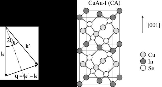
18 18 Bragg s Law One of the most famous equations in science is Bragg s law, because it is both simple and useful: dsin B = nλ Here, d is the spacing between parallel crystal planes, λ is (still) the wavelength, and B is the Bragg angle. This is not the same as the scattering angle. It is the angle that both the incident and diffracted beams make from the crystal planes. This is analogous to angles of incidence and reflection (which are also equal) referred to in optics, except in diffraction we measure the angles from the planes, not from the normal to the planes. Crystal Structure Factor We will mainly discuss scattering from crystals, and the electron scattering amplitude from a unit-cell of the crystal, rather than from individual atoms, becomes are more revealing. This sum is called the crystal structure factor, or structure factor. i F( q ) = fm ( q ) e π m atoms ( m) qd Notice that unit cell is not spherically symmetric, so we have to include vectors in the sum. The vector used is the difference between the incident and scattered wave vectors q= k -k. This length is twice that of s, so we need to use s= q when calculating form factors. Again recall we are talking about elastic scattering, so 1 k = = k = k λ A construction of the vector difference to find q also highlights the difference between and B. We can see that sin q = q = λ B In summary, ( ) F q is a sum over all constituent atoms in the crystal unit cell with appropriate phase factors for lattice positions.

19 19