UNIVERSITA` DEGLI STUDI DI PADOVA
|
|
|
- Berenice McKenzie
- 5 years ago
- Views:
Transcription

1 UNIVERSITA` DEGLI STUDI DI PADOVA SCUOLA DI INGEGNERIA Dipartimento ICEA Corso di Laurea Magistrale in Ingegneria Civile TESI DI LAUREA SOIL-STRUCTURE INTERACTION: REVIEW OF THE FUNDAMENTAL THEORIES Relatore: Prof. Roberto Scotta Correlatore: Prof. Marek Lefik Correlatore: Prof. Giampaolo Cortellazzo Laureando: Andrea Pomarè Montin Matricola: ANNO ACCADEMICO 213/214
2 Contents Preface Horizontal structures Winkler s solution Theoretical introduction Flexible beams on Winkler foundation Winkler's constant Theoretical solution - Winkler Beam on 2D model Pasternak's solution Theoretical introduction Theoretical solution Pasternak Linear elastic versus elastic plastic model Theoretical introduction Overview of the results Vertical structures Introduction Classic method - Theoretical introduction Dependent pressures method - Theoretical introduction FEM solution - Theoretical introduction Plaxis solution GeoStudio solution Overview of the results Sand Introduction: searching for the length to compare Classic Method Sand - 1 st case (9 m) results SheetPile2. Sand - 1 st case (9 m) results Plaxis Sand - 1 st case (9 m) results GeoStudio Sand - 1 st case (9 m) results Sand 1 st case (9 m) comparison Classic Method Sand 2 nd case (12 m) results SheetPile2. Sand 2 nd case (12 m) results
3 2.5.9 Plaxis Sand 2 nd case (12 m) results Plaxis No Interface Sand 2 nd case (12 m) results Sand 2 st case (12 m) comparison Overview of the results Clay Introduction: searching for the length to compare Classic Method Clay - 1 st case (1 m) results SheetPile2. Clay - 1 st case (1 m) results Plaxis Clay - 1 st case (1 m) results Plaxis No Interface Clay - 1 st case (1 m) results Clay 1 st case (1 m) comparison Classic Method Clay - 2 st case (14 m) results SheetPile2. Clay - 2 st case (14 m) results Plaxis Clay - 2 st case (14 m) results Plaxis No Interface Clay - 2 st case (14 m) results Clay 2 st case (14 m) comparison Conclusions References
4 Preface The purpose of this project is to analyze the interaction between horizontal and vertical civil structures and the soil. First, it is important to define the interaction between soil and structure : there is interaction when the response, under load, of the soil is influenced by the response of the structure, according to the stiffness and the geometrical characteristics of the latter. Horizontal structures are analyzed in the first part of this report: the theoretical introduction of Winkler s solution has been exposed and Winkler s constant was calculated by studying the trend of stresses within the ground; the adopted method allows the estimation of the stress distribution within the ground under an embankment: this issue adequately represents the plain strain model that will be used in the FEM solution; subsequently a calculation for a beam foundation has been produced (the 2D plain strain is used: the beam is a section of an infinitely extended element in the orthogonal direction to the plane of the section) using the previously found Winkler s constant applied to the differential equations for an elastic soil (implementation of solutions on a spreadsheet). Then, a comparison between analytical solutions of the beam on elastic foundation, and FEM models has been made. With FEM, elastic and elastic-plastic solutions have been compared; particular focus has been placed on the dependence between the solution and the choice of parameters, the constitutive model of the soil and of the stresses within the ground: the purpose is to understand whether the elastic model adopted in previous analysis adequately describes the issue. Alternative analytical solution of Pasternak has been illustrated and compared with the previous solutions of Winkler and FEM, then applications of this theory has been shown, both in 2D and 3D models. In the second part the focus shifts on the vertical structures: theoretical description of the methods used in the study of the behavior of sheet piles under horizontal load of the soil after excavation has been made. Simplified limit equilibrium method, numerical solution based on the theory of Winkler s elastic-plastic springs (dependent pressure) and FEM methods are used. Comparison of the solutions obtained by the different approaches has been made, distinguishing the case of an excavation in a clay soil from that in a sandy soil. For both cases the behavior of the structure has been observed, either when the embedment length widely ensures the equilibrium, also in situations close to instability: in particular the contribution that the interface element provides to the solution has been studied. The effect of the water table on the soil-structure interaction was not taken into account in this report. Aims and workflow can be summarized as follows: Analytical methods: theoretical description, implementation, results Numerical methods: description of the model, modeling, calculation 3
5 Comparison: systematic observation of the different results from different solutions, verify the compatibility of the approaches Approximation: determination of which approach better simulates the real behavior of the soil-structure model Analytical versus numerical analyses: acceptability, limits of both of them 4
6 1 Horizontal structures 1.1 Winkler s solution Theoretical introduction In order to transfer the upper load of a building or another layer into the soil, a structure is required and the purpose of this structure is to support the superstructure, avoiding the failure and having settlements inside certain acceptable limits (Figure 1). The half-space of the soil could be nonhomogeneous, anisotropic in its material, and the constitutive relations will be complex and unknown or even undeterminable, so simplifications must be taken. Figure 1: Winkler s springs The behavior of the soil is taken as linearly elastic or rigid plastic when mathematical analyses are used (Figure 2). The Boussinesq problem is when a linearly elastic material is used, that s to say where all layers have the same elastic properties. Figure 2: Winkler s model A used calculation technique refers to Winkler model, and concentrates on the behavior of the upper stiff layer, the structure, a beam usually; according to this theory the soil has only a supporting role. The continuum representation of half space can t be used for this model. The foundation material which Winkler adopted is now called Winkler foundation, and is a model substitution. In this model the pressure, p, acting at a point is equal to the deflection of the ground at that point, w, multiplied by a proportionality constant, k, so that (1) 5
7 The constant, k, is the foundation stiffness, but other used names are coefficient of subgrade reaction or subgrade modulus. Its dimensions are FL -3. The first analysis deals with the behavior of the rigid beam,: the complete problem is one of plane strain, in fact the focus could be on either a real beam of finite width b or may a strip of unit width, that s to say a typical element of a slab impressed with line loads, moments, or displacements. The situation in either of these cases is twodimensional, so the basic subgrade modulus k, to give an appropriate value for use in analysis, must be multiplied by the beam (b) or strip (1) width: (2) or (3) and has dimensions FL -3 [1]. Anyway, the focus will be on the flexible beams on Winkler foundation Flexible beams on Winkler foundation For a general description has been considered a beam of constant cross section and with its axis in the x-direction; q is the load on the beam (a force per unit length), w is the vertical displacement (in z-direction)(figure 3). Figure 3: Beam with uniform load The formulae describing the behavior of a beam are listed below. In order to respect the condition of equilibrium in z-direction (the direction perpendicular to the axis of the beam) the following condition must be satisfied (Figure 4): ( ) ( ) (4) where T is the shear force. It s been assumed that, when the force on a surface with its normal in the positive x-direction is acting in the positive z-direction, then it is conventionally positive. 6
8 The second condition to be satisfied is the equation of equilibrium of moments ( ) ( ) (5) where M is the bending moment. In this case a positive stress (tension) on the positive side of the axis of the beam it s equivalent of a positive bending moment. Figure 4: Equilibrium of a part of a beam The combination of these two equations gives the first basic equation of the theory of bending of moments ( ) ( ) (6) It s been applied the Bernoulli s hypothesis for the plane cross sections of the beam (it remains plane after deformation) and it s been assumed that the rotation dw/dx is small compared to one. In this way it s possible to obtain the second basic equation of the theory of bending of moments which concerns the deformation of the beam ( ) ( ) (7) where EI is the flexural rigidity of the beam. The combination of these two equations gives the basic equation of the classical theory of bending of beams, a fourth order differential equation for the lateral displacement 7
9 ( ) ( ) (8) Figure 5: Beam on elastic soil The external load and the soil reaction are considered the lateral load in case of a beam resting on an elastic foundation (Figure 5). As a first approximation it s possible to assume that the soil reaction is equal to the lateral displacement multiplied by the subgrade modulus k, and in this case the differential equation is ( ) ( ) ( ) (9) ( ) ( ) ( ) (1) with typical substitution (11) leads to the Winkler s formula ( ) ( ) ( ) (12) The form of the solution of the homogeneous equation (when q = ) is ( ) ( ( ) ( )) (( ) ) ( ( ) ( )) (13) [2] [3]. 8
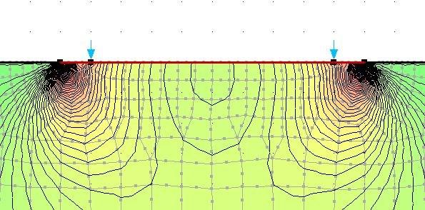
10 1.1.3 Winkler's constant The first target to be achieved is the Winkler's constant k. On a spreadsheet a general situation of double layer of soil has been created, the first one is composed of sand (coarse soil), and the second one of clay (fine soil). The characteristics of the materials have been chosen so as to be absolutely generic. These are the values: Table 1: Soil s parameters SAND - COARSE CLAY - FINE T1 E1 c'1 φ'1 ν1 T2 E2 c'2 φ'2 ν2 [kpa] [kpa] [ ] [-] [kpa] [kpa] [ ] [-] The layers have a depth of 5 meters each, and above the first layer there is a concrete beam foundation with general characteristics. Two concentrated forces act on the beam (Figure 6), but for this topic they are considered as distributed force on the surface: it is a strong approximation, because the two models are different. In the next chapters the solution with two forces on the beam has been considered more adequate for the analysis, hence this first schematization has been considered acceptable, considering the stiffness of the beam that allows to estimate the foundation as a rigid element. The dimension of the beam and the magnitude of the force have been varied so as to have an interpretation of the behavior of the Winkler's k. Figure 6: Loaded beam According to find the k for a particular combination of forces and dimensions, the layers have been divided in substrates and in each one the stress has been calculated using the formula adopted to estimate the trend of stress under an embankment: this issue, as said in the preface, properly describes the plain strain model which is implemented in the FEM programs that will be adopted in the following chapters 9
11 (the beam is a section of an infinitely extended foundation in the orthogonal direction to the plane of the section). The formula (14) could be substituted by Navfac s abacus (1982) [4], and it is usually used for the calculation of stresses under embankments (Figure 7). Figure 7: Stress under an embankment [4] [ ( )] (14) Figure 8: The analyzed model From the stress, the displacement for each substrate has been estimated and, accordingly, the total displacement has been calculated. Finally the k has been obtained from the ratio between the pressure on the beam and the displacement. Below the parameters (Table 2) adopted in the spreadsheet, the ground settlement w and k are listed: the latter is the value which will be used in the further calculations. 1
12 Table 2: Parameters for the calculation of "k" w k H B L L/B A P1 P2 q [kn/m 3 ] [-] [m 2 ] [kn] [kn] [kn/m] As illustrated in the table, the settlements that will be considered in the following calculations are the ones obtained with L/B = 1 m, P1 = P2 = 1 kn and q = (P1 + P2) /L = 2 kn/m. A graphic (Figure 9) has been created to illustrate the variation of the stress under the foundation varying the depth and the load on the beam. Δσ v Z/B [-] Δσ v [kpa] q=2kpa q=1kpa q=67kpa q=5kpa q=4kpa q=2kpa Figure 9: Stress distribution varying the pressure on the ground Theoretical solution - Winkler On a new spreadsheet, according to simulate the behavior of the beam on Winkler's springs, have been used the values taken from the previous spreadsheet obtained with a 1 meters beam with two forces of 1 kn each acting 1 m inside the two edges. According to simplify the structure the beam has been divided into two parts of 5 meters each, with boundary conditions that respect the former situation of forces and constraints. The new beam rests on the Winkler's springs obtained from the previous spreadsheet and has been divided into fifty parts, and for each part has been calculated the settlement obtained with the formula from Winkler's theory of the beam on elastic soil, and for the same part has been calculated from the first to the fourth derivative of the previous formula. In this way is easy to calculate the settlement, the shear force, bending moment and rotation in each part of the beam. As said before, it s been considered only half-beam, the left one: to find the solution one need to adopte k, in this case it s been used the k obtained by the former spreadsheet adopted for the stress calculation. 11
13 Figure 1: Border conditions for Winkler s solution Solution of the beam on the left-hand side of point of application of the force: ( ) ( ( ) ( )) (( ) ) ( ( ) ( )) (15) Solution of the beam on the right-hand side of point of application of the force: ( ) ( ( ) ( )) (( ) ) ( ( ) ( )) (16) Conditions for the eight constants. On the right end of the beam (telescope): ( ( ) ) (17) ( ) ( ) (18) At the section of action of the force: ( ( ) ) ( ( ) ) (19) ( ( ) ) ( ( ) ) (2) ( ) ( ) ( ) ( ) (21) 12
14 ( ) ( ) ( ) ( ) (22) On the left end of the beam: ( ( ) ) (23) ( ( ) ) (24) Have been created graphics to show the trend of these variables (bending moment, shear force, displacement) along the beam, and the tables illustrate the main values of the beam. Table 3: Parameters of the beam C1_1 C2_1 C3_1 C4_1 C1_2 C2_2 C3_2 C4_ H B L L1 L2 E J [kpa] [m 4 ] EJ λ λ*l k P1 P2 Δx [knm 2 ] [m -1 ] [-] [kn/m 3 ] [kn] [kn] Tmax Tmin Mmax Mmin Wmax Wmin [kn] [kn] [knm] [knm] [w] [w] Displacement w(x) Displacement x Figure 11: Displacement (analytical) 13
15 2 Bending Moment 15 M(x) [knm] 1 5 Bending Moment x Figure 12: Bending moment (analytical) T(x) [kn] Shear Force x Shear Force Figure 13: Shear force (analytical) Beam on 2D model The results obtained with the analytical model, that's to say from mathematical solution, are compared with the ones from 2D models done by GeoStudio FEM program. The soil has been assumed as linear elastic material (chapter 1.3.1): the parameters are the Young s modulus E, the self-weight γ and the Poisson s ration ν. Also the cohesion and friction angle are taken into account as data in this model: they aren t used in the solution but the Contour program uses them as well as Mohr- Coulomb failure criterion to better illustrate yield regions; in fact in this way the lack of a yield value, that cannot be defined in a linear elastic model and could cause unrealistic strains in the calculation, is filled, and the theoretical yield stresses may be compared visually with shear stresses obtained by the calculation [5]. 14
16 Table 4: Parameters of the soils and of the beam SAND CLAY H γ ν Es H γ ν Es [kn/m 3 ] [-] [kpa] [kn/m 3 ] [-] [kpa] x x1 3 BEAM Eb L A J P1 P2 q [kpa] [m 2 ] [m 4 ] [kn] [kn] [kn/m] 3x In the following chapters different models of the same problem will be analyzed and a comparison between them will be made First model Beam 1 The first model is based on a beam of 1 meters resting on two layers of soil, 5 meters of depth each, with the same characteristics of the analytical model. The length of the two layers is 3 meters (for a good approximation it s necessary to have at least the same meters of the length of the beam on the right and on the left). The boundary conditions are applied to the borders of the whole macro region, and they fixed the x and y displacements on the base, and fixed the x displacement on the sides. In the following graphics it s possible to check the differences between this model and the analytical one. A different approach to the discretization has been also considered: in fact first has been made a model ( rough version ) in which the discretization is not accurate, so the results are not acceptable. Then a refined model has been made: it uses a good discretization, and gives acceptable results. The other two models ( 1 st and 2 nd discretization) show that the previous discretization doesn t need other improvements (that could cause an increase of the computational effort), and is sufficient to describe the situation. The mesh is different according to the level of discretization used, and for the same reason also the size of the elements has been modified in the points where the accuracy of the solution could be increased. In the following examples each level of discretization will be more widely explained Rough version The mesh has 341 nodes and 3 elements and is composed by 4-noded quadrilaterals and 3-noded triangles, thus the integration points (and the integration orders) are four and three respectively; the approximate global element size is 1 m. There is no increase of discretization at strategic points or along the beam. This mesh has been automatically generated by the program. In this case it s 15

 can t give adequate information regarding")

17 easy to see how a too simple model gives unacceptable results: the aim is to have an accurate distribution of displacement, bending moment and shear force on the beam: the 4-noded quadrilaterals and 3-noded triangles (default element) can t give adequate information regarding the behavior of the beam element. Figure 14: Mesh beam 1 Rough version -A Figure 15: Mesh beam 1 Rough version -B Figure 16: Displacement beam 1 Rough Version 16


18 Y-Displacement (m) Soil structure interaction: review of the fundamental theories Figure 17: Total stress YY beam 1 Rough version The mesh is too large, too simple, and because of this the graphics of bending moment, shear force and displacement aren t precise. Figure 18: Discretization beam 1 Rough version Displacement X (m) Figure 19: Displacement beam 1 Rough version 17
19 Shear Force (kn) Moment (kn-m) Soil structure interaction: review of the fundamental theories 5 4 Bending Moment X (m) Figure 2: Bending moment beam 1 Rough version 4 3 Shear Force Figure 21: Shear force beam 1 Rough version The problems are more evident for the shear force because it is the third derivative of the displacement, so the error is bigger Refined version X (m) In this model, secondary nodes have been applied to the mesh elements, and their integration order has been increased; the mesh has been generated along the line of the beam, decreasing the size of the mesh elements under the beam and near the most important points of the latter: the edges and the forces application points. This level of discretization will also be used in the next models. The mesh contains 1434 nodes and 453 elements, and is composed of 8-noded quadrilaterals and 6-noded triangles, thus the integration points (and the integration orders) are four (with nine Gauss points the element would be too rigid) and three respectively; the approximate global element size is 1 m. 18


20 Figure 22: Mesh beam Refined version -A Figure 23: Mesh beam Refined version -B Figure 24: Mesh particular A-B, Beam Model Figure 25: Discretization of mesh A-B 19


21 Figure 26: Discretization of mesh C-D Figure 27: Displacement Beam 1 Refined version Figure 28: Total Stress YY Beam 1 Refined version This better discretization gives better results; in fact the graphics are much more precise. Figure 29: Discretization Beam 1 Refined version 2
22 Shear Force (kn) Moment (kn-m) Y-Displacement (m) Soil structure interaction: review of the fundamental theories Displacement X (m) Figure 3: Displacement beam 1 Refined version 8 Bending Moment X (m) Figure 31: Bending moment beam 1 Refined version 6 Shear Force X (m) Figure 32: Shear force beam 1 Refined version 21


 are four and three respectively; the approximate global")

23 st discretization It is quite evident that this discretization does not significantly affect the results of the previous model; this means that the former model was rather accurate: such an accurate discretization is excessively high. The mesh has 5479 nodes and 1778 elements and is composed by 8-noded quadrilaterals and 6-noded triangles, thus the integration points (and the integration orders) are four and three respectively; the approximate global element size is.5 m. The computational effort is high and unnecessary. Figure 33: Mesh 1 st discretization A Figure 34: Mesh 1 st discretization B Figure 35: 1 st discretization particular A-B 22

 Figure 38: Bending moment beam 1 1 st discretization")
24 Moment (kn-m) Y-Displacement (m) Soil structure interaction: review of the fundamental theories Figure 36: Discretization Beam 1, 1 st discretization Displacement X (m) Figure 37: Displacement beam 1 1 st discretization 8 Bending Moment X (m) Figure 38: Bending moment beam 1 1 st discretization 23


25 Shear Force (kn) Soil structure interaction: review of the fundamental theories 6 Shear Force X (m) Figure 39: Shear force beam 1 1 st discretization nd discretization This discretization is a little less precise than the refined one, but nevertheless not so different to have completely incompatible results. The mesh has 459 nodes and 149 elements and it is composed by 8-noded quadrilaterals and 6-noded triangles, thus the integration points (and the integration orders) are four and three respectively; the global element size is 2 m. Figure 4: Mesh 2 nd discretization A Figure 41: Mesh 2 nd discretization A 24


 Figure")
26 Y-Displacement (m) Soil structure interaction: review of the fundamental theories Figure 42: 2 nd discretization particular A-B Figure 43: Discretization Beam 1, 2nd discretization Displacement X (m) Figure 44: Displacement beam 1 2 nd discretization 25
27 Shear Force (kn) Moment (kn-m) Soil structure interaction: review of the fundamental theories 6 Bending Moment X (m) Figure 45: Bending moment beam 1 2 nd discretization 6 Shear Force X (m) Figure 46: Shear force beam 1 2 nd discretization Comparison of results from various discretizations In these graphics it s possible to check how the difference between the last three models is not significant: on the contrary the first rough model is too simple. After this comparison the refined version has been chosen as the most suitable to describe the problem, and it is also cost effective for the computational calculation. Regarding the displacement in the right hand side of the beam, it s interesting to notice the difference between 1 st discretization, refined and 2 nd discretization, probably due to a numerical error. 26
28 Displacement 5 1 w(x) st discretization 2nd discretization Rough Refined -.72 x Figure 47: Displacement, different discretization M(x) [knm] Bending Moment 5 1 x 1st discretization 2nd discretization Rough Refined Figure 48: Bending foment, different discretization T(x) [kn] Shear Force 5 1 x 1st discretization 2nd discretization Rough Refined Figure 49: Shear force, different discretization 27
29 Comparison with analytical result Considering the refined version as the correct solution for the 1 st model a comparison between the analytical solution and that obtained with GeoStudio has been made. -.2 Displacement w(x) Analytical Beam1_GeoStudio -.12 x Figure 5: Displacement, Analytical-beam 1 GeoStudio M(x) [knm] Bending Moment 5 1 x Analytical Beam1_GeoStudio Figure 51: Bending Moment, Analytical -beam 1 GeoStudio 28
![T(x) [kn] 8 6 4 2-2 -4-6 -8-1 Shear Force 2 4 6 8 1 x Analytical Beam1_GeoStudio Figure 52](/docs-images/82/86583395/images/30-0.jpg ": Shear force, Analytical -beam 1 GeoStudio 1.1.5.")

30 T(x) [kn] Shear Force x Analytical Beam1_GeoStudio Figure 52: Shear force, Analytical -beam 1 GeoStudio Second model Beam 2 The second model represent half beam, that's to say 5 meters only, and as boundary condition on the section of division it's been created a proper beam, a link, with a stiffness of an order of magnitude more than that of the previous beam, in this way the conditions of the complete beam are fulfilled. The soil below the beam is divided into two layers of 5 meters each, the characteristics are the same of the previous examples. The solution completely matches the previous one, thus it hasn t been represented. Figure 53: Mesh beam 2, rigid link 1, rigid link 2 29
31 Y-Displacement (m) Soil structure interaction: review of the fundamental theories Third model Beam 3N The third model (where N is for normal ) is completely different from the former ones, because in this case hasn't been used the soil below the 1 m beam, but the beam is free. In order to have the same conditions of the soil this beam has as boundary conditions, in addition to the forces, Winkler's springs acting on each node of the beam. The constant of the springs is the one obtained from the analytical model: the influence length of the concentrated spring is 1 m. In this model and in all the models with springs, the bending moment has opposite values compared to those of the solution with no springs due to the sign convention: consequently, in the comparison with the other solutions the diagram of the aforementioned stress parameter has been inverted. These are the results. Figure 54: Mesh beam 3N, trick Displacement X (m) Figure 55: Displacement beam 3N 3
32 Shear Force (kn) Moment (kn-m) Soil structure interaction: review of the fundamental theories 2 BendingMoment X (m) Figure 56: Bending moment beam 3N 8 6 Shear Force X (m) Figure 57: Shear force beam 3N Comparison with analytical result As for the previous chapter the following graphics compare the analytical solution and Geostudio; in order to have a suitable comparison between the two solutions the bending moment s diagram obtained with GeoStudio will be inverted. 31
33 -.95 Displacement w(x) Analytical Beam3N_GS x Figure 58: Displacement, Analytical-beam 3N GeoStudio 2 Bending Moment M(x) [knm] x Analytical Beam3N-inverse_GS Figure 59: Bending moment, Analytical-beam 3N GeoStudio 1 Shear Force 5 T(x) [kn] Analytical Beam3N_GS -1 x Figure 6: Shear force, Analytical-beam 3N GeoStudio 32
34 Y-Displacement (m) Soil structure interaction: review of the fundamental theories Fourth model Beam 3BD The fourth model (where BD is for better discretization ) is the same of the previous one, but with a better discretization: in fact each spring is applied on an area of.1 cm multiplied by 1 m, so the value of the k of each spring is equal to the value of the former k divided by ten. The solution is shown below. Figure 61: Mesh beam 3BD -.16 Displacement X (m) Figure 62: Displacement beam 3BD 33
35 Shear Force (kn) Moment (kn-m) Soil structure interaction: review of the fundamental theories 2-2 BendingMoment X (m) Figure 63: Bending moment beam 3BD 8 6 Shear Force X (m) Figure 64: Shear force beam 3BD Comparison with analytical result Graphics with a comparison between the results obtained with the analytical solution and with GeoStudio will be proposed. As for the former chapter the bending moment s diagram obtained with GeoStudio will be inverted. These solutions match almost perfectly because both of them adopt the same k, and because the distribution of the springs along the beam is thicker. 34
36 w(x) Displacement x Analytical Beam3BD_GS Figure 65: Displacement, Analytical-beam 3BD GeoStudio 2 Bending Moment M(x) [knm] x Analytical Beam3BDinverse_GS Figure 66: Bending moment, Analytical-beam 3BD GeoStudio T(x) [kn] Shear Force x Analytical Beam3BD_GS Figure 67: Shear force, Analytical-beam 3BD GeoStudio 35
37 Y-Displacement (m) Soil structure interaction: review of the fundamental theories Fifth model Beam 4N The fifth model (where N is for normal ) represents the same situation of the third, but only half beam with a link as boundary condition (as the second model) has been created, the springs replace the soil. The results are the following. Figure 68: Mesh beam 4N, rigid link Displacement X (m) Figure 69: Displacement beam 4N 36
38 Shear Force (kn) Moment (kn-m) Soil structure interaction: review of the fundamental theories 2 Bending Moment X (m) Figure 7: Bending moment beam 4N Shear Force X (m) Figure 71: Shear force beam 4N Comparison with analytical result As for the former chapters, a comparison between the solution obtained with analytical solution and the one obtained with GeoStudio will be proposed. As in the previous graphics the GeoStudio s bending moment s diagram will be inverted. 37
39 w(x) Displacement x Analytical Beam4N_GS Figure 72: Displacement, Analytical-beam 4N GeoStudio 2 Bending Moment M(x) [knm] x Analytical Beam4N-inverse_GS Figure 73: Bending moment, Analytical-beam 4N GeoStudio T(x) [kn] Shear Force x Analytical Beam4N_GS Figure 74: Shear force, Analytical-beam 4N GeoStudio 38
40 Y-Displacement (m) Soil structure interaction: review of the fundamental theories Sixth model Beam 4BD The sixth model has the same characteristics of the fifth one (half beam on springs), but the discretization is the same as the one adopted to the third model (springs every.1 m). Figure 75: Mesh beam 4BD -.17 Displacement X (m) Figure 76: Displacement beam 4BD 39
41 Shear Force (kn) Moment (kn-m) Soil structure interaction: review of the fundamental theories 2-2 Bending Moment X (m) Figure 77: Moment 4BD 4 Shear Force X (m) Figure 78: Shear force beam 4BD Comparison with analytical result In this section a comparison between the solution obtained with GeoStudio and the one obtained with the analytical solution will proposed. As in the previous graphics the GeoStudio s bending moment s diagram will be inverted. 4
42 w(x) Displacement x Analytical Beam4BD_GS Figure 79: Displacement, Analytical-beam 4BD GeoStudio 2 Bending Moment M(x) [knm] x Analytical Beam4BD-inverse_GS Figure 8: Bending moment, Analytical-beam 4BD GeoStudio T(x) [kn] Shear Force x Analytical Beam4BD_GS Figure 81: Shear force, Analytical-beam 4BD GeoStudio 41
43 Comparison In the following graphics it s possible to compare all the models with the one obtained with the analytical solution. The results of the models that take into account the springs match the analytical one because in these for the springs have been used the same value of k used for the analytical solution, on the contrary the models with real layers of soil use the parameters required for the linear-elastic analysis and not k. The only case which differs is Beam 3N regarding the displacement, probably because of the low discretization; fact that is replied regarding the shear force with Beam 3N and Beam 4N. Displacement w(x) Beam1 Beam3N Beam3BD Beam4N -.1 Beam4BD -.12 x Analytical Figure 82: Displacement, different models Bending Moment 2 M(x) [knm] x Beam1 Beam3N-inverse Beam3BD-inverse Beam4N-inverse Beam4BD-inverse Analytical Figure 83: Bending moment, different models 42
44 1 Shear Force T(x) [kn] x Beam1 Beam3N Beam3BD Beam4N Beam4BD Analytical Figure 84: Shear force, different models 1.2 Pasternak's solution Theoretical introduction Pasternak created a model a little more complex than the Winkler s one. As for the Winkler s model, it s important to understand how the soil deformation influences the behavior of the beam. One can notice that the stress at the interface and the soilbeam interaction depend on the geometrical characteristics of the beam and on the mechanical properties (elastic) of the soil. The Pasternak solution takes into account both the soil below the beam and the soil next to it (Figure 85): this is an obvious difference from Winkler s model, in which only the loaded region under the beam settles, while the adjacent surface remains unchanged. The soil nearby the beam forms a wave due to the deformation and because the material is a connected continuum. Pasternak created a model to get sag which qualitatively describes this behavior. Figure 85: Pasternak s behavior of the soil It is assumed that the reaction at each point of the ground under the beam is in proportion to the displacement of the ground at that point (Winkler setting), but this component of the reaction depends on the curvature of the beam at that point. The constant of proportionality is the modulus of soil stiffness, the Winkler s k. 43
45 The curvature coefficient is used for the reaction coefficient (S) introduced by Pasternak, and it s interpreted as a traction force under the beam (slab) provided by a fictitious membrane placed between the beam (slab) and the soil. Pasternak model has two parameters (not only λ, but also α and β). Other assumptions are chosen without changing the scheme of the Winkler beam: movement of the beam and displacement of the ground are the same only when the soil is compressed and, only in special cases, when it is in traction. In the formulation of the problem is not taken into account the possibility of a difference between the displacement of the beam and the movement of the soil. The description can be as follows: a membrane layer between the ground and the beam (thick gray line in the Figure 86). This layer is a "diaphragm" which is placed in traction by a constant force S that acts in the tangential direction to the membrane surface. The vertical resultant force acts on the bottom of the beam (or plate). It s possible to analyze the linear section of the diaphragm (black section in the Figure 86): Figure 86: Membrane behavior The sum of projections on the tangential axis to the membrane results in: (25) because dl = Rγ where R is the local radius of curvature, one can write: (26) 44
46 The inverse of the curvature radius is approximately equal to the second derivative of the deflection line. The relationship between the pressure force resulting from the curvature of the beam and the force of the "membrane" is shown as follows: (27) This extra load is a supplement to the Winkler s model and leads to the following equations. Starting from the equilibrium equations of the beam: ( ) ( ) (28) where M is the bending moment, p is the load perpendicular to the axis of the beam: the axis the of the beam is oriented to the x-direction. We take into account the Winkler assumption, total load on the ground is p, distributed load is q and soil reaction is r = -kw(x). ( ) ( ) ( ) ( ) (29) ( ) ( ) ( ) ( ) (3) If EI (flexural stiffness of the beam, E Young's modulus of the beam s material, I moment of inertia about the axis of the center) is independent of x, we can obtain a simple equation: ( ) ( ) ( ) ( ) (31) 45
47 ( ) ( ) ( ) ( ) (32) with the typical substitution: (33) leads to the Pasternak s formula: ( ) ( ) ( ) ( ) (34) particular solution of the equation (with zero on the right) (which is easy to check by substitution) is of the form: ( ) ( ( ) ( )) (( ) ) ( ( ) ( )) (35) (36) (37) S is a concentrated force ([kn]) that already takes into account the membrane thickness and the width of the interval (for example, the width of the beam B). If one want to check, for S = is obtained the solution of the Winkler equation. Complete solution is obtained by adding any specific solution. If q(x) is (as usual) solid (or solid pieces), it is a particular solution and is, as before, in Winkler, the following: 46
48 (38) Note further that, in accordance with the intuitive interpretation, one may assume that the solution of the "membrane" refers to the surface of the ground "outside" the beam. This is important because in the case of ground covered by an actual membrane (geosynthetics) the equation outside the beam is as follows: ( ) ( ) ( ) (39) The solution of this equation is the special form: ( ) (4) Coefficient k is the coefficient of Winkler, calculated as it was shown before. The S coefficient has a simple interpretation of the "strength of the membrane." Unfortunately, this membrane is fictitious. Therefore, S is a highly speculative factor. Even if the membrane was real (geostucture), unfortunately, the S factor is still difficult to determine, because it can be interpreted as the strength of the membrane and therefore it would be part of the solution task and not the output value. The problem gets "non-linear", and a method of trial and correction is required. Starting from the theory of elastic half-space, the resultant of the horizontal stress that occur within the soil when the area under the beam (plate) is compressed can be calculated. Figure 87: Pasternak s model S is the resultant of the layer with a certain thickness H. 47
49 The Figure 87 above shows the intuitive cooperation of the land beyond the line of the foundation. According to the method of Vlasov and Leontiev, the following formula it has been obtained (commonly, also different formulae are used, giving similar results): ( ) (41) g is a function describing the change in the vertical displacement with the depth. One can take g from the formula: ( ) (42) where μ can be reasonably taken as a constant. E is Young's modulus, ν is Poisson's ratio. In practice, the condition to be fulfilled is: (43) Assuming the lower limit for μ one obtains: (44) Using geosynthetics (membrane, geogrid) under the foundation, the classical solutions is not correct (geosynthetics have 1, max 2 years). Pasternak model could be useful in that application but in this case S is a part of the solution: nevertheless the value of S per unit of width ( B ) can be is easily found [6] Theoretical solution Pasternak In the example the same beam used on the Winkler s soil has been considered, but on the left-hand side there is a new element, the fictitious geosynthetic. For this part the formulae shown in the previous pages have been used. The boundary conditions are different from the Winkler s ones. 48
50 Under consideration, the left half-beam and the soil with the fictitious geosynthetic: in order to find the solution one need to calculate k, to adopt S and then calculate α and β. Figure 88: Border conditions of Pasternak s solution Solution of the beam on the left-hand side of point of application of the force: ( ) ( ( ) ( )) (( ) ) ( ( ) ( )) (45) Solution of the beam on the right-hand side of point of application of the force: ( ) ( ( ) ( )) (( ) ) ( ( ) ( )) (46) Solution on the left, for the "membrane": ( ) (47) Conditions for the ten constants: on the right end of the beam (telescope): ( ( ) ) (48) ( ) ( ) (49) At the section of action of the force: 49
51 ( ( ) ) ( ( ) ) (5) ( ( ) ) ( ( ) ) (51) ( ) ( ) ( ) ( ) (52) ( ) ( ) ( ) ( ) (53) On the left end of the beam: ( )( ) ( )( ) (54) ( ) ( ) ( ( ) ) (55) ( ( ) ) (56) The last condition is satisfied placing: (57) in this way, the curve tends to infinity on the left side. In the following graphics it is possible to notice the comparison between the solution obtained with Winkler and with Pasternak; three different outputs of the Pasternak s solution changing the value of S have been illustrated: the first is obtained with the previous formula, the second is obtained placing S = 1 kn, the third obtained placing S = 1 kn. The results that obtained with GeoStudio are more similar to the ones obtained with the Pasternak s model (analytical) than the ones obtained with Winkler (analytical) (Figure 89): in particular the Pasternak s model simulates with good accuracy the behavior of the soil nearby the beam, the bending moment and the shear force. With S= 1 kn Pasternak s model (analytical) matches the solution of Winkler (analytical), that s to say that the membrane doesn t work (Figure 92). 5
52 Table 5: Parameters for the calculation with Pasternak (analytical); the implemented values is for the case S calc C1_M C2_M C1_1 C2_1 C3_1 C4_1 C1_2 C2_2 C3_2 C4_ H B L L1 L2 E J EJ λ λ*l [kpa] [m 4 ] [knm 2 ] [m -1 ] [-] α β E1 ν S S*SENθ k P1 P2 Δx [m -1 ] [m -1 ] [kpa] [-] [kn] [kn] [kn/m 3 ] [kn] [kn] Tmax Tmin Mmax Mmin Wmax Wmin [kn] [kn] [knm] [knm] Displacement w(x) Winkler_Analytical Beam 1_GeoStudio Pasternak S calc -.12 x Figure 89: Displacement obtained with Winkler (analytical), GeoStudio (FEM), Pasternak (analytical) 2 Bending Moment 15 M(x) [knm] x Winkler_Analytical Beam 1_GeoStudio Pasternak S calc Figure 9: Bending moment obtained with Winkler (analytical), GeoStudio (FEM), Pasternak (analytical) 51
53 T(x) [kn] Shear Force x Winkler_Analytical Beam 1_GeoStudio Pasternak S calc Figure 91: Shear force obtained with Winkler (analytical), GeoStudio (FEM), Pasternak (analytical) Displacement.2 w(x) Winkler_Analytical Beam 1_GeoStudio Pasternak S calc Pasternak S= x Pasternak S=1 Figure 92: Displacement obtained with Winkler (analytical), GeoStudio (FEM), Pasternak (analytical) M(x) [knm] Bending Moment x Winkler_Analytical Beam 1_GeoStudio Pasternak S calc Paternak S=1 Pasternak S=1 Figure 93: Bending moment obtained with Winkler (analytical), GeoStudio (FEM), Pasternak (analytical) 52
54 T(x) [kn] Shear Force x Winkler_Analytical Beam 1_GeoStudio Pasternak S calc Pasternak S=1 Pasternak S=1 Figure 94: Shear force obtained with Winkler (analytical), GeoStudio (FEM), Pasternak (analytical) w(x) Displacement x Pasternak S calc Pasternak S=1 Pasternak S=1 Figure 95: Displacement obtained with Winkler (analytical), GeoStudio (FEM), Pasternak (analytical) 15 Bending Moment 1 M(x) [knm] x Pasternak S calc Paternak S=1 Pasternak S=1 Figure 96: Bending moment obtained with Winkler (analytical), GeoStudio (FEM), Pasternak (analytical) 53
55 T(x) [kn] Shear Force x Pasternak S calc Pasternak S=1 Pasternak S=1 Figure 97: Shear obtained with Winkler (analytical), GeoStudio (FEM), Pasternak (analytical) As it is easy to see, the solution with the Pasternak model (analytical) using the S calculated with the equation (44) better simulates the behavior of the continuum solution (GeoStudio, FEM) than the Winkler s solution (analytical). Pasternak model is useful to describe this kind of situation (long beam resting on elastic soil), but it is also helpful to study some interesting application that will be shortly described Pasternak Symmetrical solution In this application has been considered a symmetrical situation of a soil, with a distributed load applied on it to a length of 2 meters, and half a meter of free soil (not loaded) beside the two edges of the loaded soil: this model could describe the behavior of a loaded membrane (real as geosynthetics, or fictitious) resting on an elastic soil. The equations that describe the behavior of the membrane and of the ground around are the same used in chapter of the theoretical beam (in addiction there is the distributed load), but with some simplifications caused by the symmetry: in fact the equation of the membrane needs only two constants of integration (and not two for half membrane and other two for the other half)), and as for the free soil the equation needs one constant (no more two, that s to say the same situation of the theoretical beam) because in that way the displacement curve tends to infinite on the far side of the piece of soil, so the other constant can be placed equal to zero. This simplification provides a computational advantage. On the left side of the loaded membrane the equation is ( ) (58) 54
56 and the equation of the unloaded part, left side, is ( ) (59) On the right side of the loaded membrane the equation is ( ) (6 ) and the equation of the unloaded part, right side, is ( ) (61) where k is the subgrade modulus and S is the membrane force. Conditions for the four constants: on the left end of the loaded area: ( )( ) ( )( ) (62) ( ) ( ) ( ) ( ) (63) On the right end of the loaded area: ( )( ) ( )( ) (64) The last condition is satisfied placing: [7]. (65) In the following graphics the trend of the displacement in function of k, q and S will be illustrated: for the values of k have been chosen the results of the previous calculations by the Winkler s method plus two arbitrary values of k = 5 kn/m 3 and k = 1 kn/m 3. 55
57 Table 6: Parameters for the solution; the implemented values are the chosen ones for one of the analyzed cases L k φ'1 S q P1 P2 P1+P2 Δx [kn/m 3 ] [ ] [kn] [kn/m] [kn] [kn] [kn] C1_M C2_M C3_M w(x) Displacement (S) - Winkler - q = x Winkler kw-s=1 kw-s=1 kw-s=1 kw-s=1 kw-s=1 Figure 98: Displacement of the membrane varying S, k assumes the value adopted in the Winkler s solution and indicated in Table 6, q = 1 kn/m Displacement (S) - k1 - q = 1.5 w(x) x k=5 k-s=1 k-s=1 k-s=1 k-s=1 k-s=1 Figure 99: Displacement of the membrane varying S, k1 = 5 kn/m 3, q = 1 kn/m 56
58 Displacement (s) - k2 - q = 1.2 w(x) x k=1 k-s=1 k-s=1 k-s=1 k-s=1 k-s=1 Figure 1: Displacement of the membrane varying S, k1 = 1 kn/m 3, q = 1 kn/m w(x) Displacement (k) - S =1 - q = x k=1-s=1 k=1-s=1 k=1-s=1 k=1-s=1 k=1-s=1 Figure 11: Displacement of the membrane varying k, S = 1 kn, q = 1 kn/m Displacement (k) - S =1 - q = w(x) k=1-s=1 kw-s=1 k=5-s=1-2 x Figure 12: Displacement of the membrane varying k, S = 1 kn, q = 1 kn/m 57
59 Displacement (q) - Winkler - S= w(x) x kw-q=1 kw-q=1 kw-q=1 Figure 13: Displacement of the membrane varying q, k assumes the value adopted in the Winkler s solution and indicated in Table 6, S = 1 kn Displacement (q) - Winkler - S= w(x) x kw-q=1 kw-q=1 kw-q=1 Figure 14: Displacement of the membrane varying q, k assumes the value adopted in the Winkler s solution and indicated in Table 6, S = 1 kn Pasternak Reinforced soil This example considers a part of ground of 3 m of length, with a distributed load applied on it. The soil has two different subgrade moduli: in fact on the two edges of this piece of ground, for.5 m on each side, has a ten times greater stiffness than the soil in the middle. This distribution of stiffness tries to simulate the situation that is possible to find when are used gravel columns in the soil, or piles, but always materials with greater stiffness than the soil. The geometry and the loads are symmetrical, so one can imagine a description similar to the one used in the previous chapter, with similar simplifications and advantages. As in the previous case, the model can show the behavior of a loaded membrane resting on an elastic 58
60 soil (with two different stiffnesses). So the equations that describe this application are the same used before, with the accuracy of using two different k. The simplifications caused by the symmetry permit to consider only half of the area (1.5 m), only two constants of integration for the part with "normal soil" and only two for the "reinforced soil" (so have been found the constants only for half of the considered zone, because in the other part the constants are the same because of the symmetry). On the left side of the loaded membrane resting on the normal soil the equation is ( ) (66) and the equation of the reinforced part, left side, is ( ) (67) On the right side of the loaded membrane resting on the normal soil the equation is ( ) (68) and the equation of the reinforced part, right side, is ( ) (6 9) where k is the subgrade modulus for the normal soil, kf the subgrade modulus for the reinforced soil and S is the membrane force. Conditions for the four constants: on the left end of the loaded area on the normal soil: ( )( ) ( )( ) (7) ( ) ( ) ( ) ( ) (71) On the right end of the loaded area on the normal soil: ( ) ( ) (72) 59
61 On the left end of the loaded area on the reinforced soil: [7]. ( ) ( ) (73) As in the previous application the following graphics illustrate the trend of the displacement in function of k, q and S: the results of the previous calculations by the Winkler s method plus two arbitrary values of k (k = 5 kn/m 3, k = 1 kn/m 3 ) have been used as k for the comparison. Table 7: Parameters for the solution; the implemented values are the chosen ones for one of the analyzed cases L k kf φ'1 S q P1 P2 P1+P2 [kn/m 3 ] [kn/m2] [ ] [kn] [kn/m] [kn] [kn] [kn] C_1 C_2 C_3 C_ E-6 w(x) Displacement (S) - Winkler - q = x Winkler kw-s=1 kw-s=5 kw-s=1 kw-s=2 kw-s=3 kw-s=5 kw-s=1 Figure 15: Displacement of the membrane varying S, k assumes the value adopted in the Winkler s solution and indicated in Table 7, q = 1 kn/m 6
62 w(x) Displacement (S) - k1 - q = x k=5 k-s=1 k-s=5 k-s=1 k-s=2 k-s=3 k-s=5 k-s=1 Figure 16: Displacement of the membrane varying S, k1 = 5 kn/m 2, q = 1 kn/m w(x) Displacement (S) - k2 - q = x k=1 k-s=1 k-s=5 k-s=1 k-s=2 k-s=3 k-s=5 k-s=1 Figure 17: Displacement of the membrane varying S, k2 = 1 kn/m 2, q = 1 kn/m Displacement (k) - S =1 - q = w(x) x k=1-s=1 k=1-s=1 k=1-s=1 Figure 18: Displacement of the membrane varying k, S = 1 kn, q = 1 kn/m 61
63 w(x) Displacement (k) - S =1 - q = x Figure 19: Displacement of the membrane varying k, S = 1 kn, q = 1 kn/m w(x) x Figure 11: Displacement of the membrane varying k, S = 1 kn, q = 1 kn/m w(x) Figure 111: Displacement of the membrane varying q, k assumes the value adopted in the Winkler s solution and indicated in Table 7, S = 1 kn 62 k=1-s=1 k=1-s=1 k=1-s=1 Displacement (k) - S =1 - q = x k=1-s=1 kw-s=1 k=5-s=1 Displacement (q) - Winkler - S= 1 kw-q=1 kw-q=1 kw-q=1
64 w(x) Displacement (q) - Winkler - S= Figure 112: Displacement of the membrane varying q, k assumes the value adopted in the Winkler s solution and indicated in Table 7, S = 1 kn Pasternak Finite difference x kw-q=1 kw-q=1 kw-q=1 The third and probably most remarkable example deals with the situation analyzed in the second example but extended in a 2D loaded area, with deformative effects along the third axis (3D). First of all the equation of the membrane is similar to the one used in the previous chapter, but in this case represents a surface in two variables: ( ( ) ( ) ) ( ) ( ) (74) where w is the displacement, k the subgrade modulus, q the load, S the membrane force. This equation can be easily solved with the finite difference method applied on a spreadsheet. The 2D area the area has the shape of a square of 3 m from the side; in each of the four corners there is a square of.5 m from the side that represents the soil with greater stiffness (piles, gravel columns). The second derivative of a function f(x) can be approximated in this way: ( ) (75) ( ) ( ) ( ) ( ) (76) where is the center, h the step, Δ the variation. 63
, L, C, R, D, U (respectively left, central, right, down, up) are the values of w in the cells nearby (and in) a selected cell, k is the subgrade modulus, S the")
65 The equation of the membrane has a second partial derivative, so the solution used in the spreadsheet is a little more complicated: ( ( ) ( )) (77) where Δx is placed equal to Δy (the discretization of the membrane along the two axis), L, C, R, D, U (respectively left, central, right, down, up) are the values of w in the cells nearby (and in) a selected cell, k is the subgrade modulus, S the membrane force, w and q are considered constants in the selected cell. In the cells where the stiffness is greater (in the corners) kf takes the place of k in the equation. The equation of the membrane is valid in all the area, exept to the borders. Thus all the cells among the border must be placed equal to the cells that have (respectively) on the inner side of the left. This application has circular references, but you can set spreadsheet to find an iterative solution [7]. The 3D-graphics show the behavior of the membrane varying q, k (the value of k is the one obtained by the Winkler s method plus an arbitrary value of k = 1 kn/m 3 ) and S. Table 8: Parameters for the solution; the implemented values are the chosen ones for one of the analyzed cases q delta kw kf S cm cf p [kn/m2] [kn/m 3 ] [kn/m 3 ] [kn/m] [-] [-] w(x,y) w(x,y) - q = 1^4 - k = 1^3 - S = 1^ Figure 113: Displacement of the membrane for q = 1 kn/m, k = 1 kn/m 3, S = 1 kn/m 64
.")
 - q = 1^4 - kw - S = 1^3 -.5.5-1 1-1.5 1.5-2 2-2.5 2.5-3 3-3.5 3.5-4 4-4.5 4.")
66 w(x,y) w(x,y) - q = 1^2 - k = 1^3 - S = 1^ Figure 114: Displacement of the membrane for q = 1 kn/m, k = 1 kn/m 3, S = 1 kn/m w(x,y) w(x,y) - q = 1^4 - kw - S = 1^ Figure 115: Displacement of the membrane for q = 1 kn/m, k assumes the value adopted in the Winkler s solution and indicated in Table 8, S = 1 kn 65


67 w(x,y) w(x,y) - q = 1^2 - kw - S = 1^ Figure 116: Displacement of the membrane for q = 1 kn/m, k assumes the value adopted in the Winkler s solution and indicated in Table 8, S = 1 kn/m w(x,y) w(x,y) - q = 1^2 - kw - S = 1^ Figure 117: Displacement of the membrane for q = 1 kn/m,, k assumes the value adopted in the Winkler s solution and indicated in Table 8, S = 1 kn/m 66

68 w(x,y) w(x,y) - q = 1^2 - k = 1^3 - S = 1^ Figure 118: Displacement of the membrane for q = 1 kn/m, k = 1 kn/m 3, S = 1 kn/m 1.3 Linear elastic versus elastic plastic model Theoretical introduction In this chapter will be introduced a new FEM program in order to analyze the same problem studied in the former chapters, but changing the constitutive model from linear elastic into elastic-plastic: the program is Midas GTS, and the adopted constitutive model is Mohr-Coulomb. The purpose is to highlight the differences that occur between the two models, focusing on the behavior of the soil changing the constitutive parameters and in particular understand if the choice of the elastic model for the former analyses is suitable or not; that s to say that in the following chapter it has been verified until which value of the ratio between the load and the strength of the material an elastic model could be replace an elastic-plastic model. Linear elastic model is the simplest constitutive model, its coefficients are the elastic modulus E and the Poisson s ratio ν. In 3D analysis the stress-strain relationship is expressed by the equation (78). ( )( ) (78) { } { } [ ] 67
69 In 2D analyses τyz = τzx = γyz = γzx =, and especially for plain strain analyses εz =. The parameter ν represents the pure volumetric strain, and as it approaches.5 the volumetric strain becomes close to (incompressibility): in order to not have numerical problems is programs usually the assumed value is ν =.49. In this model the strain is directly proportional to the stress (Figure 119); the slope of linear curve is constant and depending on E and ν. Figure 119: Stress-strain relationship of linear elastic model [8] Generally the elastic model describes the behavior of the soil immediately after the load is applied and for small deformation. This method based on the Hook s Law is highly used for simple and preliminary analysis. The stress-strain relationship of soil is very complex: it depends on the material composition, porosity, stress history and loading method and exhibits a nonlinear material characteristics: it is very difficult to approximate soil as an elastic material. For this reason the key parameter, E, must be clearly defined to adequately replace the real behavior of soil. Linear elastic analysis usually refers to deformability of the ground whereas elasticplastic analysis refers either to deformability or instability of ground. Instability is determined by the shear strength of a material, deformability by both shear strength and elastic properties. If the load is greater of the shear strength capacity of the ground, some areas could reach the failure limit (plastic state), confined yield zones, surrounded by elastic zones; anyway some local failures do not necessarily cause a global failure. An elastic-plastic model distinguishes between reversible (elastic) and irreversible (plastic) deformation. The yield function defines the stress-condition at which deformation may occur. If the yield function is not satisfied the deformations will be fully elastic. 68
70 In the stress-strain relationship of an elastic and perfectly plastic model the stress is directly proportional to strain until the yield point after which the curve becomes completely horizontal (Figure 12). Figure 12: Stress-strain relationship of elastic-plastic model [8] The parameters that define the model are the elastic modulus E, the Poisson s ratio ν, the cohesion c, the friction angle φ, the dilatancy angle ψ. Usually the deformation caused by a load is composed by components: elastic and plastic strain. (79) Where ε is the total strain, ε e is the elastic strain, ε p is the plastic strain. Some concepts are important to define the constitutive equations in plasticity: yield criteria (set the starting point of plastic deformation), flow rule (define plastic deformation), hardening rule (define deformation hardening) The yield function (or loading function), F, which defines the limit of the elastic response range of a material is defined: ( ) ( ) ( ) (8) In plasticity theory the yield function can t be a positive value. When yielding occurs, the stress state is modified by accumulating plastic strains until the yield function is reduced to zero. This process is known as the Plastic Corrector phase or Return Mapping. Where σ, σe, k, ε p are the current stress, the equivalent or effective stress, hardening factor, equivalent plastic strain respectively. 69
71 The plastic deformation that uses the plastic rule shown in is expressed by the following equations: (81) Where g/ σ is the direction of plastic straining and dλ the plastic multiplier that defines the magnitude of plastic straining. Figure 121: Geometric illustration of associated flow rule and singularity [8] The function g is the Plastic potential, usually defined in terms of stress invariants. If g is equal to F it is termed as Associated flow rule and the direction of the plastic strain vector is orthogonal to the yield surface; if g and F are unequal it is referred as Non-associated flow rule. The former can be expressed by the following equation: (82) Special consideration is required if singular points (Figure 121) occur at a corner or flat surface (impossibility to define the plastic flow path). The equation (83) is the standard constitutive equation. Stress increments are determined by the elastic part of the strain increments. ( ) ( ) (83) Where D e is the elastic constitutive matrix. The following consistency condition needs to be satisfied so as the stresses are always maintained on the yield surface. Therefore the equation (93) allows to calculate the infinitesimal stress increments. 7
72 ( ) (84) Using the full Newton-Raphson iteration procedure and a consistent stiffness matrix the convergence can be much faster due to the second-order convergence characteristic of the aforementioned method. Where ( ) (85) ( ) (86) ( ) (87) In the elastic-plastic analyses carried out in this chapter (and also using GeoStudio and Plaxis in chapter 2) the Mohr-Coulomb failure criterion (19) has been adopted; it is expressed by: τ (σ) (88) The limiting stress state, τs, in a plane is only related to the normal stress, σ, in the same plane. The failure envelope expressed by the equation (88) is experimentally determined. The Mohr s criterion affirms that a material fails when the largest Mohr s circle is tangent to the envelope. For this reason no effect on the failure condition is due to the intermediate principal stress σi (σ1, σ2, σ3). The straight line defined by equation (89) represents the simplest representation of the Mohr s failure envelope: τ σ φ (89) Where c is the cohesion and φ the friction angle. The Mohr-Coulomb failure criterion is usually described by the equation (98). There are three limitations in using the Mohr-Coulomb criterion. Firstly, when the failure envelope is reached by the largest Mohr s circle the intermediate principal stress σi (σ1, σ2, σ3) doesn t influence the failure stress: this is inconsistent with experimental results. Secondly, the meridians and failure envelop of the Mohr s circle are straight lines and independent of strength parameter (φ) and hydraulic (or confining) pressure (Figure 122)Figure 122:: the precision of the criterion is 71
 at the corner. Lastly, the Mohr-Coulomb cannot describe the compaction of soil.")
73 good for limited hydraulic pressure, but it decreases by increasing the hydraulic pressure area. Numerical errors may occur due to the discontinuity of the yield surface (that is not smooth) at the corner. Lastly, the Mohr-Coulomb cannot describe the compaction of soil. Figure 122: Schematization of yield function [9]. Despite this limitations, adopting this criterion within practical hydraulic pressure limits leads to relatively good results; it is a widely used criterion to model granular materials (such as soil and concrete) due to its precision and simplicity and has been successfully used in geotechnical engineering; assuming this model the solutions in nonlinear analyses are reliable. The Mohr-Coulomb equation can also be expressed in terms of the principle stresses (σ1 σ2 σ3), in terms of stress invariants J1, J2 and θ, or in terms of the variables ξ, ρ and θ. Figure 123: The Mohr-Coulomb yield surface in principal stress space (c=) [1] 72
74 In the following chapter the applications of this model will be carried out [9], [8], [1] Overview of the results In this chapter have been analyzed the behavior of the same model studied in chapter but adopting an elastic plastic constitutive model. The aim is to verify if the previous model is adequate to describe the system of loaded beam resting on the soil for the given set of conditions. The used program is Midas GTS. Table 9: Parameters of the soils and of the beam (Mohr-Coulomb constitutive model) SAND H γ φ c ν ψ Es K [kn/m 3 ] [ ] [kpa] [-] [ ] [kpa] [-] x1 3.5 CLAY H γ φ c ν ψ Es K [kn/m 3 ] [ ] [kpa] [-] [ ] [kpa] [-] x1 3.5 BEAM Eb L A J P1 P2 q [kpa] [m 2 ] [m 4 ] [kn] [kn] [kn/m] 3x The mesh is composed by 4-noded quadrilateral elements (four integration points) and 3-noded triangular elements (one integration point), that s to say linear elements with linear interpolation. The first type of elements leads to accurate displacement and stress result, whereas the second type provides poor accuracy of stresses, the displacements are good: the geometry and the system beam-loads is not so detailed or complex, so these elements are suitable to the problem, furthermore the use of quadratic elements could lead to a rigid behavior not consistent with the real soil. The used analyses is construction stage, that s to say that first the in situ analysis has been performed by using the K method which allows to determine the stresses within the soil caused by the self-weight of ground before the activation of loads, then the displacements (by choosing an option in the program) have been deleted (in fact a new parameter which wasn t considered in the elastic method is the non-dimensional quantity K = σh / σv, where σh and σv the horizontal and the vertical stress within the ground respectively). The second step is the activation of the loads and the consequent analysis. 73


: the purpose is to verify if the behavior of the soil is still elastic or turned into elastic-plastic, in the latter case the")
75 The iteration method adopted is the Newton-Raphson method, the load increment is the equidistant load step, the convergence criterion is force norm ratio : all these parameters are summarized in Figure 124. Figure 124: Midas GTS analysis set up A comparison between elastic model and elastic-plastic model (both performed by Midas GTS) have been performed, by using for the second type a cohesion c =.1 Kpa (the value causes numerical error in the calculation of the stiffness matrix), and by varying the entity of loads (from two forces of 1 kn each to two forces of 2 kn each): the purpose is to verify if the behavior of the soil is still elastic or turned into elastic-plastic, in the latter case the model assumed in chapter would be incorrect. In the following graphics (Figure 125, Figure 126) one can see the displacement of the beam for both elastic and elastic-plastic case (with c =.1 kpa) by varying the entity of load. 74
76 Displacement y x LE_F=1kN LE_F=2kN LE_F=5kN LE_F=1kN LE_F=2kN LE_F=5kN EP_F=1kN LE_F=2kN Figure 125: Displacement of the beam on linear elastic soil by varying the entity of load y Displacement -3.5 x EP_F=1kN EP_F=2kN EP_F=5kN EP_F=1kN EP_F=2kN EP_F=5kN EP_F=1kN EP_F=2kN Figure 126: Displacement of the beam on elastic-plastic soil (c=.1 kpa) by varying the entity of load As it is easy to see for the load F = 1 kn (that s to say two forces of 1 kn each), the assumed load in chapter, the behavior seems to be similar either for elastic or elastic-plastic model. In order to prove this hypothesis the displacement of two nodes along the symmetry axis of the beam has been calculated: the load has been varied with the same modality as the previous analysis, both for the elastic model that the elastic-plastic model. The first point is located 1 m below ground level (in the sandy soil), the second 6 m below the ground level (in the clay soil). The following force-displacement graphics (from Figure 127 to Figure 131) illustrate the trend of the solution. One can see the level of plasticity of soil in the following screenshots from Figure 132 to Figure 135: in the first image only some plastic points appear under the right force (one can notice the asymmetry of the response 75
77 of the soil, probably because of a numerical error in the post processing procedure, Figure 132) under a load of two forces of 1 kn each. In the second image (Figure 133) appear the first plastic points in the clay soil under a load of two forces 6 kn each. In the third image (Figure 134) appear plastic points around the node (in clay) considered in the analysis (6 m below the ground level, along the axis of symmetry of the beam) under a load of two forces of 2 kn each. The fourth image shows the spread of plasticity in the clay soil under a load of two forces of 5kN each. For this reason it s possible to say that the behavior of the point of in clay is elastic until a load of two forces of 2 kn is applied when plasticity occurs. From the graphics force-displacement the point in sand seems to behave like the one in sand, that s to say that is seems to gradually plasticize: in the screenshots this phenomenon doesn t appear, probably because a numerical error in the post processing procedure. Anyway the important achievement is that the soil (sand and clay) is surely in an elastic state for a load of two forces of 1 kn each and consequently the model used in the chapter is suitable to characterize the issue described Force -Displacement 15 1 F [kn] Sand_-1m_EP Clay_-6m_EP 5 Sand_-1m_LE Clay_-6m_LE w Figure 127: Force-displacement graphic of the two points in sand and clay, linear elastic constitutive model and elastic-plastic constitutive model 76
78 25 2 Force -Displacement F [kn] Sand_-1m_EP Sand_-1m_LE w Figure 128: Force-displacement graphic of the point in sand, linear elastic and elastic-plastic constitutive model 25 2 Force -Displacement F [kn] Clay_-6m_EP Clay_-6m_LE w Figure 129: Force-displacement graphic of the point in clay, linear elastic and elastic-plastic constitutive model 77
79 25 2 Force -Displacement F [kn] Sand_-1m_LE Clay_-6m_LE w Figure 13: Force-displacement graphic of the two points in sand and clay, linear elastic constitutive model 25 2 Force -Displacement F [kn] Sand_-1m_EP Clay_-6m_EP w Figure 131: Force-displacement graphic of the two points in sand and clay, elastic-plastic constitutive model 78


80 Figure 132: Plastic points under a load of two forces of 1 kn each Figure 133: Plastic points under a load of two forces of 6 kn each Figure 134: Plastic points under a load of two forces of 2 kn each 79
 screenshots of some characteristics of the model will be shown in the following pages; in addiction for every load with graphics will be shown the trend of the displacement of")
. Increasing the load the soil diverges from the elastic behavior, and consequently the displacement and the stress increase.")
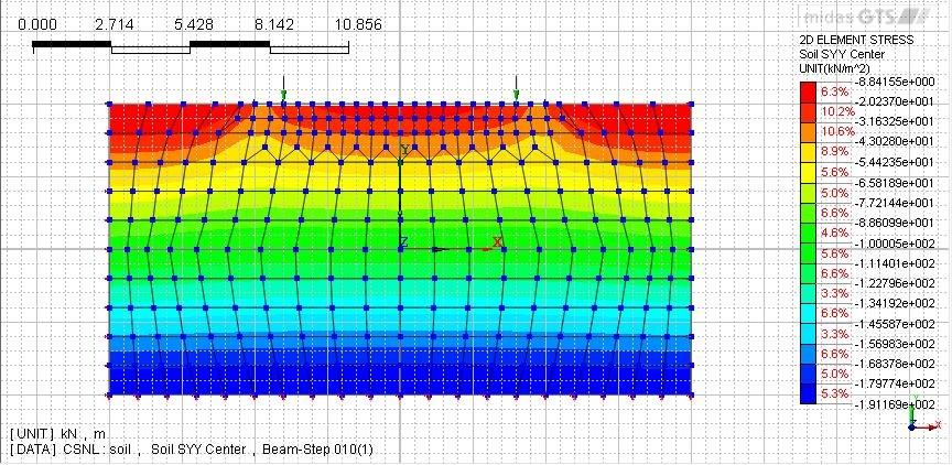
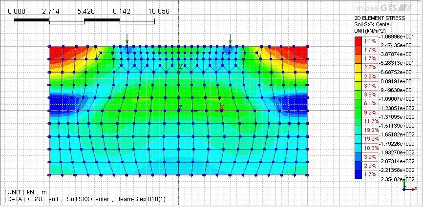
81 Figure 135: Plastic points under a load of two forces of 5 kn each In order to have a whole description of the behavior of the points of in sand and clay under the three topic loads described before (1 kn, 2 kn and 5 kn) screenshots of some characteristics of the model will be shown in the following pages; in addiction for every load with graphics will be shown the trend of the displacement of the beam, the displacement of the points along the axis of symmetry, the stress SYY below the left force, the mid-point of the beam, the right either for the elastic model or for the elastic-plastic one varying the cohesion (from c =.1 kpa to 2 kpa). Increasing the load the soil diverges from the elastic behavior, and consequently the displacement and the stress increase. The variation of the cohesion modifies the response of the soil but not significantly than the elastic model. Remarkable is the trend of the bending moment and of the shear force of the beam (from Figure 175 to Figure 177): as for the other characteristics of the model also this stress parameters diverge from the elastic solution. Figure 136: Displacement DY, F=1 kn, linear elastic 8


82 Figure 137: Bending moment, F=1 kn, linear elastic Figure 138: Shear force, F=1 kn, linear elastic Figure 139: Stress SXX, F=1 kn, linear elastic 81


83 Figure 14: Stress SYY, F=1 kn, linear elastic Figure 141: Displacement DY, F=1 kn, elastic plastic, c=.1 kpa Figure 142: Bending moment, F=1 kn, elastic plastic, c=.1 kpa 82


84 Figure 143: Shear force, F=1 kn, elastic plastic, c=.1 kpa Figure 144: Stress SXX, F=1 kn, elastic plastic, c=.1 kpa Figure 145: Stress SYY, F=1 kn, elastic plastic, c=.1 kpa 83


85 Figure 146: Displacement DY, F=2 kn, linear elastic Figure 147: Bending moment, F=2 kn, linear elastic Figure 148: Shear force, F=2 kn, linear elastic 84


86 Figure 149: Stress SXX, F=2 kn, linear elastic Figure 15: Stress SYY, F=2 kn, linear elastic Figure 151: Displacement DY, F=2 kn, elastic plastic, c=.1 kpa 85


87 Figure 152: Bending moment, F=2 kn, elastic plastic, c=.1 kpa Figure 153: Shear force, F=2 kn, elastic plastic, c=.1 kpa Figure 154: Stress SXX, F=2 kn, elastic plastic, c=.1 kpa 86


88 Figure 155: Stress SYY, F=2 kn, elastic plastic, c=.1 kpa Figure 156: Displacement DY, F=5 kn, linear elastic Figure 157: Bending moment, F=5 kn, linear elastic 87


89 Figure 158: Shear force, F=5 kn, linear elastic Figure 159: Stress SXX, F=5 kn, linear elastic Figure 16: Stress SYY, F=5 kn, linear elastic 88
90 Figure 161: Displacement DY, F=5 kn, elastic plastic, c=.1 kpa Figure 162: Bending moment, F=5 kn, elastic plastic, c=.1 kpa Figure 163: Shear force, F=5 kn, elastic plastic, c=.1 kpa 89


91 Figure 164: Stress SXX, F=5 kn, elastic plastic, c=.1 kpa Figure 165: Stress SYY, F=5 kn, elastic plastic, c=.1 kpa 9
92 w(x) Displacement x Elastic EP_C=.1 EP_C=.2 EP_C=.5 EP_C=1 EP_C=2 EP_C=5 EP_C=1 EP_C=15 w(x) Displacement x EP_C=.1 EP_C=.2 EP_C=.5 EP_C=1 EP_C=2 EP_C=5 EP_C=1 EP_C=15 EP_C= y Displacement_Mid w(y) Elastic EP_C=.1 EP_C=.2 EP_C=.5 EP_C=1 EP_C=2 EP_C=5 EP_C=1 EP_C=15 Figure 166: Displacement of the beam and of the nodes along the axis of symmetry, F=1 kn 91
93 σ yy [kpa] σ yy _y = -.5 m x Elastic EP_C=.1 EP_C=.2 EP_C=.5 EP_C=1 EP_C=2 EP_C=5 EP_C=1 EP_C=15 σ yy [kpa] σ yy _y = -2.5 m x Elastic EP_C=.1 EP_C=.2 EP_C=.5 EP_C=1 EP_C=2 EP_C=5 EP_C=1 EP_C=15 σ yy [kpa] σ yy _y = -7.5 m x Elastic EP_C=.1 EP_C=.2 EP_C=.5 EP_C=1 EP_C=2 EP_C=5 EP_C=1 EP_C=15 Figure 167: Stress SYY calculated at.5 m, 2.5 m, 7.5 m below the ground level, F=1 kn 92
94 y σ yy [kpa] σ yy _Fsx Elastic EP_C=.1 EP_C=.2 EP_C=.5 EP_C=1 EP_C=2 EP_C=5 EP_C=1 EP_C=15 y σ yy [kpa] σ yy _Mid Elastic EP_C=.1 EP_C=.2 EP_C=.5 EP_C=1 EP_C=2 EP_C=5 EP_C=1 EP_C=15 y σ yy [kpa] σ yy _Fdx Elastic EP_C=.1 EP_C=.2 EP_C=.5 EP_C=1 EP_C=2 EP_C=5 EP_C=1 EP_C=15 Figure 168: Stress SYY calculated below the left force,the mid-point of the beam,the right force, F=1 kn 93
95 w(x) Displacement x Elastic EP_C=.1 EP_C=.2 EP_C=.5 EP_C=1 EP_C=2 EP_C=5 EP_C=1 EP_C=15 w(x) Displacement x EP_C=.1 EP_C=.2 EP_C=.5 EP_C=1 EP_C=2 EP_C=5 EP_C=1 EP_C=15 EP_C=2 y Displacement_Mid w(y) Elastic EP_C=.1 EP_C=.2 EP_C=.5 EP_C=1 EP_C=2 EP_C=5 EP_C=1 EP_C=15 Figure 169: Displacement of the beam and of the nodes along the axis of symmetry, F=2 kn 94
96 σ yy [kpa] σ yy _y = -.5 m x Elastic EP_C=.1 EP_C=.2 EP_C=.5 EP_C=1 EP_C=2 EP_C=5 EP_C=1 EP_C=15 EP_C=2 σ yy [kpa] σ yy _y = -2.5 m x Elastic EP_C=.1 EP_C=.2 EP_C=.5 EP_C=1 EP_C=2 EP_C=5 EP_C=1 EP_C=15 EP_C=2 σ yy _y = -7.5 m σ yy [kpa] x Elastic EP_C=.1 EP_C=.2 EP_C=.5 EP_C=1 EP_C=2 EP_C=5 EP_C=1 EP_C=15 EP_C=2 Figure 17: Stress SYY calculated at.5 m, 2.5 m, 7.5 m below the ground level, F=2 kn 95
97 y σ yy [kpa] σ yy _Fsx Elastic EP_C=.1 EP_C=.2 EP_C=.5 EP_C=1 EP_C=2 EP_C=5 EP_C=1 EP_C=15 EP_C=2 y σ yy [kpa] σ yy _Mid Elastic EP_C=.1 EP_C=.2 EP_C=.5 EP_C=1 EP_C=2 EP_C=5 EP_C=1 EP_C=15 EP_C=2 y σ yy [kpa] σ yy _Fdx Elastic EP_C=.1 EP_C=.2 EP_C=.5 EP_C=1 EP_C=2 EP_C=5 EP_C=1 EP_C=15 EP_C=2 Figure 171: Stress SYY calculated below the left force, the mid-point of the beam, the right force, F=2 kn 96
98 Displacement w(x) x Elastic EP_C=.1 EP_C=.2 EP_C=.5 EP_C=1 EP_C=2 EP_C=5 EP_C=1 EP_C=15 EP_C=2 w(x) Displacement x EP_C=.1 EP_C=.2 EP_C=.5 EP_C=1 EP_C=2 EP_C=5 EP_C=1 EP_C=15 EP_C=2 y Displacement_Mid w(y) Elastic EP_C=.1 EP_C=.2 EP_C=.5 EP_C=1 EP_C=2 EP_C=5 EP_C=1 EP_C=15 Figure 172: Displacement of the beam and of the nodes along the axis of symmetry, F=5 kn 97
99 σ yy [kpa] σ yy _y = -.5 m x Elastic EP_C=.1 EP_C=.2 EP_C=.5 EP_C=1 EP_C=2 EP_C=5 EP_C=1 EP_C=15 σ yy [kpa] σ yy _y = -2.5 m x Elastic EP_C=.1 EP_C=.2 EP_C=.5 EP_C=1 EP_C=2 EP_C=5 EP_C=1 EP_C=15 σ yy [kpa] σ yy _y = -7.5 m x Elastic EP_C=.1 EP_C=.2 EP_C=.5 EP_C=1 EP_C=2 EP_C=5 EP_C=1 EP_C=15 Figure 173: Stress SYY calculated at.5 m, 2.5 m, 7.5 m below the ground level, F=5 kn 98
100 y σ yy [kpa] σ yy _Fsx Elastic EP_C=.1 EP_C=.2 EP_C=.5 EP_C=1 EP_C=2 EP_C=5 EP_C=1 EP_C= y σ yy [kpa] σ yy _Mid Elastic EP_C=.1 EP_C=.2 EP_C=.5 EP_C=1 EP_C=2 EP_C=5 EP_C=1 EP_C= y σ yy [kpa] σ yy _Fdx Elastic EP_C=.1 EP_C=.2 EP_C=.5 EP_C=1 EP_C=2 EP_C=5 EP_C=1 EP_C=15 Figure 174: Stress SYY calculated below the left force, the mid-point of the beam, the right force, F=5 kn 99
101 M(x) [knm] Bending Moment x Elastic EP_C=.1 EP_C=.2 EP_C=.5 EP_C=1 EP_C=2 EP_C=5 EP_C=1 EP_C=15 EP_C=2 Shear Force T(x) [kn] x Elastic EP_C=.1 EP_C=.2 EP_C=.5 EP_C=1 EP_C=2 EP_C=5 EP_C=1 EP_C=15 EP_C=2 Figure 175: Bending moment and shear force, F=1 kn 1
102 M(x) [knm] Bending Moment x Elastic EP_C=.1 EP_C=.2 EP_C=.5 EP_C=1 EP_C=2 EP_C=5 EP_C=1 EP_C=15 EP_C= T(x) [kn] Shear Force -15 x Elastic EP_C=.1 EP_C=.2 EP_C=.5 EP_C=1 EP_C=2 EP_C=5 EP_C=1 EP_C=15 EP_C=2 Figure 176: Bending moment and shear force, F=2 kn 11
103 M(x) [knm] Bending Moment x Elastic EP_C=.1 EP_C=.2 EP_C=.5 EP_C=1 EP_C=2 EP_C=5 EP_C=1 EP_C=15 EP_C= T(x) [kn] Shear Force -4 x Elastic EP_C=.1 EP_C=.2 EP_C=.5 EP_C=1 EP_C=2 EP_C=5 EP_C=1 EP_C=15 EP_C=2 Figure 177: Bending moment and shear force, F=5 kn [11], [12], [13], [8]. 12
104 2 Vertical structures 2.1 Introduction The interaction between soil and structure can also be studied in vertical elements, such as sheet pile retaining walls. In this case the interaction is very complicated because the soil has the dual purpose of loading the structure on the active side of the sheet pile and support it on the passive side, in fact it has a portion embedded in the soil. That s why a part from the FEM techniques, the other kind of methods are based on empirical or empirically based factors and a theoretically correct solution can t be achieved. The design of a retaining wall needs two sets of calculation, one to achieve the equilibrium of the structure, the other to determine, from the values of bending moments and shear forces obtained from equilibrium, the characteristics of the structure. Generally retaining walls can be divided into two categories: cantilever and supported walls. The first type requires a sufficient embedment, that s to say the fixity of the toe, and this attribute depends on the penetration into the ground. The second type, either tied or strutted, shares the supporting role between soil and supporting members. Usually the effectiveness of a cantilever depends on its acceptable deflection under load. The height determines whether it is more effective a cantilever or a propped wall. The design of the wall must be carried out taking into account either the Ultimate Limit State or the Serviceability Limit State: the latter is important when the deflection of the wall and the movement of the ground are significant. The designer has also to decide either to use free earth model or fixed earth model for the toe of the wall, and the difference between the two assumptions is based on the influence that the depth of embedment has on the wall deflection. A wall designed as a free earth support behaves like a supported vertical beam, the toe is allowed to rotate and not to translate; a tie or a prop on the top could be the other support; this kind of model, for a given set of conditions, requires less depth of embedment but the beam has a maximum for bending moment. A fixed earth support avoids either translation or rotation of the toe, so it acts like a propped cantilever (fixed end); the upper support could be provided by a prop or a tie. In this case the maximum bending moment along the beam decreases but the toe fixity creates a fixed end moment in the wall and an increase of the depth of embedment of the beam is required. This design approach must be adopted when the end of the sheet pile is fixed and the embedment in the soil provides the support of the wall. No failure mechanism exists to check the stability of the sheet piles once the fixed earth support is assumed, but many empirical approach have been studied. Both methods are valid only if support is provided over the middle of the retained height. 13
105 An important topic of wall design is the distribution of pressures and the bending moment reduction. In fact the triangular distribution of earth pressure is a simplification that doesn t take into account the interaction between soil and structure, feature that influences the distribution of bending moments and shear forces along the wall, and of earth pressure itself. The soil and the flexibility of the wall influence this reduction and this deflection of the wall causes a movement away from the soil (between the embedded part and the position of the support). This movement could cause an arching effect within the soil: the internal capabilities are improved and the pressure on the wall decreases. A reduction of the maximum bending moment and an increase of the reaction in the support obviously occurs: in fact, usually, the reaction calculated by a soil structure interaction is higher than that obtained by a limit equilibrium analysis. This arching effect could not be taken into account (or can be but with caution) in vibrational situation, stratified soils, yielding of the support or movement of the toe. Programs based on soil-structure interaction automatically take into account the arching effect on bending moment, thus for a calculation by simple equilibrium is it recommended to increase the load of a certain percentage on the support. Anyway the pressure on the wall that is commonly assumed, with its simplified triangular shape, doesn t take into account the movement of the wall (this lack nevertheless gives a conservative solution), which caused a decrease of pressure where it is large, and an increase where it is small: features that can be seen with a computer program. The shape of pressure can be further improved by a program based on the interaction between soil and structure, and the modification would be an increase of the passive pressure and a decrease of the active. As said previously it s also important to keep in mind that the deflection is a function either of the section and the material of the wall or the compression of the soil in a passive/active state: that s to say that a stiff wall with less props could be as effective as a flexible wall with more props. Thus when the soil-structure interaction is taken into account a flexible wall solution could be more cost effective than one based on a stiff wall, because a reduction in strength demand occurs so the required bending moment section is minimized [14]. In this chapter will be described some different approaches that can be used to study a retaining sheet pile wall. The first will be the classic method, it is highly simplified but can give some general indication about the length of the wall. A second approach will be a computational program based on dependent pressures. The last approach will be an analysis done with two FEM programs. The case study will be an excavation by a sheet pile: the parameters of the soil and of the structure have been chosen in an arbitrary manner and only for schematic purpose, the water table is not taken into account. Each approach will analyze two different conditions: a granular soil and a cohesive soil, for both of them will be offered a comparison between the different assumed methods. 14
106 All these descriptions will be made in the proper chapters. 2.2 Classic method - Theoretical introduction The aim of this method is to find the required length of the wall to achieve equilibrium of the structure: the soil has been assumed to be at the yielding limit state so the theory of Rankine for rigid-plastic material has been assumed. The adopted failure criterion for the soil is that of Mohr-Coulomb. The vertical pressure in the ground is: ( ) (9) where q is the load [kn/m 2 ], hi the thickness of the layer, γi the self-weight of the i-th layer; for a system where there are layers of soil below the water table (it won t be take into account in this work) shall be used the effective weight expressed by the formula: (91) where γh2o is the self-weight of water (assumed 9.81 kn/m 3 ). The active horizontal pressure is calculated by the following formula: (92) In this formula σv is the vertical stress from the weight of the soil, c is the cohesion, and Ka is the coefficient of Rankine active pressure. It amounts to: ( ) (93) where φ is the angle of internal friction of the soil. The passive horizontal pressure is: (94) 15
107 where σv and c are as above the vertical stress from the weight of the soil and the cohesion respectively; Kp is the coefficient of Rankine passive pressure. It amounts to: ( ) (95) where φ is the angle of internal friction of the soil. This method has been applied to the problem under consideration using a spreadsheet. As said before, the purpose is to achieve equilibrium by varying the length of the wall, that s to say by trial and correction. One enters the value of the depth of embedding in the spreadsheet: immediately the bending moment about the toe is calculated: the length can be assumed as correct when passive moment is slightly greater than the active moment. Where the area of the active pressure below the ground level is equal to the area of the passive pressure below the ground level, the shear force is equal to zero. The sum of the values of the bending moments about and above the level of zero shear gives the value of maximum bending moment. With the spreadsheet it s also possible to have the trend of the bending moment along the wall. A suggestion for the design in order to find the proper penetration depth of the pile is to increase by 2% the depth below the point where passive and active pressure are equal. [7], [15], [14]. 2.3 Dependent pressures method - Theoretical introduction This approach assumes that the soil in the vicinity of the wall behaves as ideally elastic-plastic Winkler material; the method is based on the Winkler model of subgrade reaction modulus that characterizes the behavior of the material in the elastic region: by exceeding the limit of deformation that occurs when passive pressure is reached, the soil behaves as ideally plastic material; the parameter kh is the stiffness on an ideal elastic support, so as for the horizontal beam, and a system of these springs replaces the reaction of the soil in contact with the wall. It has been assumed that the wall is an elastic beam and the horizontal elastic reaction of the soil is equal to the horizontal displacement at that point multiplied by kh: (96) And ( ) (97) 16
108 The kh parameter isn t the Winkler coefficient for horizontal foundation, it doesn t have a physical meaning and it depends on the stiffness and the geometry of the wall and on the condition of the soil. As the in-situ methods can t define a value of kh, either empirical or theoretical methods have been developed, the latters based on the classic theory of elasticity: some of these are Terzaghi s method, Chadeisson and Monnet method, Menard and Bourdon method. In this work has been used a program based on Chadeisson and Monnet method: its aim is to calculate the displacement with which the soil reaches the limit of passive pressure defined by Rankine. The kh evaluated by this empirical method depends on the shear force of the soil by the parameters φ and c (the adopted failure criterion is that of Mohr-Coulomb), and on the stiffness of the wall; for given subsoil: ( ( ) ) (98) [ ] where γ is the self-weight of soil, Kp the passive pressure coefficient, K the pressure coefficient at rest, dr the characteristic displacement (.15 m), c the effective cohesion, Ap the coefficient allowing for soil cohesion, c is equal to 3 kpa The formulae used in this method to determine the pressure along the wall are the same as those used for the classic method, and the coefficient of active and passive pressure are defined by the theory of Rankine: so all the formulae showed in the chapter concerning the classic method are still valid in this one. In addition the constitutive equation of the beam with small displacement is required: ( ) ( ) (99) where x(z) is a function of displacement, M(z) is the bending moment, EI is the flexural rigidity of the beam. This formula combined with the load function ( ) ( ) (1) Gives ( ) ( ) (11) 17
109 Taking into account the elastic reaction of the soil the previous equation is extended in the following way ( ) ( ) (12) where kh is the coefficient of elasticity defined in the chapter. It has been assumed that the value of the pressure acting on the wall may vary between the two bounds of passive or active pressure, but without falling outside of them, and that the acting pressure on an undeformed structure is the pressure at rest. For a deformed structure the pressure is (13) (14) (15) where σr is the pressure at rest, kh is the modulus of subsoil reaction, w is the deformation of structure, σa is the active earth pressure, σp is the passive earth pressure. The computational procedure starts with the pressure at rest acting on the wall and the kh assigned to all the system of supports (Figure 178:). Figure 178: 1 st step of the computational procedure [7] 18
110 The following step requires that the program to check the locations at which the condition for allowable magnitudes of pressures acting on the wall is satisfied or violated. In the latter case the value of kh = has been assigned, and the wall is loaded by active or passive pressure Figure 179: 2 nd step of the computational procedure [7] The above iteration procedure continues until all required conditions are satisfied. In analyses of subsequent stages of construction the program accounts for plastic deformation of the wall. This is also the reason for specifying individual stages of construction that comply with the actual construction process. The program based on this method and used in the analyses is SheetPile2.. [7], [16], [17], [15], [18]. 2.4 FEM solution - Theoretical introduction As said before the third approach that has been used for the case study is a calculation by finite element method programs. To better understand the problems related with the modeling of soil-structure interaction the analysis has been carried out by two different programs: GeoStudio and Plaxis. The latter has been used with two different modalities. The solution is highly influenced by the modeling procedure, and elements which have been properly created to replace the interaction are the key for a better result: thus a comparison between different programs is necessary to analyze this feature. A significant issue is also the construction by stage that either in GeoStudio or in Plaxis has been taken into account. The in situ analysis for the former and the initial analysis for the latter are followed by a load-deformation analysis and a 19
111 phase-1 respectively: these two-phase analyses allow the system soil-structure to simulate the actual excavation. The first phase occurs before the excavation and the second one after it: the latter stage is based on the values of deformation and stress obtained from the former one, in this way the sequence of staged construction develops like a common time continuum. In first phase the gravity is applied to the elements through the material self-weight, in order so simulate the existing state of stress. In the second phase loads are applied as boundary conditions and the new state of stress is implemented. The simulation is performed by adding or removing elements from the mesh, that s to say activating or deactivating regions. The soil has been set as an elastic-plastic material (Mohr-Coulomb model, see chapter 1.3.1) [5], [19] Plaxis solution In Plaxis the soil has been set up as an linear elastic perfectly-plastic material, and the failure criterion that has been adopted is that of Mohr-Coulomb (chapter 1.3.1), thus the parameters that define the material are (1.3.1) the Young s modulus E [kn/m 2 ], the Poisson s ratio ν [-], the cohesion c [kn/m 2 ], the friction angle φ [ ], the dilatancy ψ [ ] The issue has been analyzed as a plane strain model, thus the finite elements have two dimensions and with two translational degree of freedom per node. Figure 18: Example of a plain strain [19] A coarse element distribution has been set up, u to have an accurate solution as a first approach: as will be explained in the following chapters this distribution will be turned into a m um requirement. The average element Ie size is assumed equal to: ( )( ) (16) 11
![Where xmax, xmin, ymax, xmin are the geometry dimensions of the mesh, and nc is a value that takes into account the global coarseness Figure 181: Global coarseness [19] The element that has been used](/docs-images/82/86583395/images/112-0.jpg "is the default 15-node triangle for the first analyses and changed into a 6-node triangle in the subsequent ones: for the first one the displacements are obtained by an interpolation of the fourth")
112 Where xmax, xmin, ymax, xmin are the geometry dimensions of the mesh, and nc is a value that takes into account the global coarseness Figure 181: Global coarseness [19] The element that has been used is the default 15-node triangle for the first analyses and changed into a 6-node triangle in the subsequent ones: for the first one the displacements are obtained by an interpolation of the fourth order, and twelve Gauss points (stress points) are involved in the numerical integration; for the second one the displacements are obtained by an interpolation of the second order, and three Gauss points (stress points) are involved in the numerical integration. The 15 node triangle provides high quality stress results for difficult problems, the 6 node triangle provides good results in standard deformation analyses. Figure 182: Distribution of nodes and Gauss points [19]. A particular element must be described with more accuracy: the interface. This peculiar feature of Plaxis has a fundamental importance in the analysis, in fact it 111
113 takes into account the soil-structure interaction. A fictitious thickness defines the material properties of this element. The elastic deformation increases with the thickness: generally a little deformation is required for an interface, but you must consider that a too little thickness may ill-condition the numerical process. The parameter of the interface is Ri: Rinter: this parameter relates the strength of the soil to the strength in the interfaces [2]; Hence, using the entered Rinter-value gives a reduced interface friction and interface cohesion (adhesion) compared to the friction angle and the cohesion in the adjacent soil [2]. The equations are: (17) (18) (19) An elastic-plastic model is used to describe the relationship between soil and structure, and the Coulomb criterion is used to distinguish the elastic behavior from the plastic one. The interface to remain elastic: (11) And to behave as a plastic material: (111) Where σn is the effective normal stress, τ the shear stress, φi and ci are the friction angle and the cohesion of the soil. The shear and compression moduli are related by the expressions: (112) (113) (114) A 15-nodes soil element is connected to the corresponding interface element by five points; thus an interface element requires two pairs of five nodes to be define (one 112
114 pair for each side). A 6-nodes soil element is connected to the corresponding interface element by three points; thus an interface element requires two pairs of three nodes to be define (one pair for each side). This element has zero thickness because in the FEM formulation two nodes pair have the same coordinates. The Newton-Cotes integration allow to obtain the stiffness matrix of the interface element; the 1-node interface element uses five Newton-Cotes stress points while the 6-node interface element uses five Newton-Cotes stress points and for both of them these coincide with a node pairs. Figure 183: Distribution of nodes and stress points on an interface element [19] This element reproduces the soil-structure interaction because allows the sliding between the two surfaces, issue that is not taken into account without the interface element because the points are chained together [19], [2] GeoStudio solution As for the previous program, in the analyses performed by GeoStudio the soil has been assumed as linear elastic perfectly-plastic material, with a Mohr-Coulomb yield criterion (chapter 1.3.1). Hence the parameters required by the model are the same as those described in the former chapter. The model is a plane strain, the same as Plaxis. The mesh is composed by 6-noded triangles, thus the integration points (and the integration orders) are three. This mesh have been chosen in order to have a homogeneous comparison with Plaxis (as said in the previous chapter the 15-nodes triangle element used for the first calculation with Plaxis will be turned to a 6-nodes triangle for the comparison with GeoStudio). The size of the elements has been modified (in some strategic points for instance) in order to have a better discretization. An interface has been generated along the structure and it describes the friction properties between soil and structure. Material properties (elastic-plastic behavior, with the parameters that are required) have been assigned to the interface. However the thickness of this element doesn t 113
115 have a physical meaning and it isn t taken into account in the solution. This interface is important for the solution, but it doesn t have the properties that are specified in Plaxis. The results indeed are highly dependent on the stiffness of the interface material and on the other parameters that will be specified in the proper chapter. In order to have a homogeneous comparison with Plaxis the parameters of the interface in GeoStudio are calculated by the suggested formulae of chapter 2.4.1, these formulae could relate the two programs [5]. 2.5 Overview of the results Sand Introduction: searching for the length to compare In order to have an uniform length of the sheet pile that allows the expected comparison, it is necessary to choose the best solution, that s to say to compare the solutions obtained by different approaches for a given set of conditions, and decide which of them could be the suitable one. The first length that provides an acceptable solution for the Classic Method is 7 m (it s important to remember that this method gives a simplified solution, so it is reasonable to use a minimum value obtained by a more precise approach). The minimum value for Sheetpile2. is 7.5 m, but the displacement is 8.43 cm. The minimum value for Plaxis is 8.5 m, but the displacement is cm (peak value). GeoStudio in this case is considered a comparison program. Plaxis provides an acceptable solution (.957 cm) with a 1 m length sheet pile, and the length to be analyzed will be chosen by varying the length of the sheet pile adopting this program. Using a 12 m length sheet pile the maximum displacement is.923 cm, from 13 m on there isn t a significant improvement of the performance. In order to compare two different behaviors have been chosen two different comparison lengths for the sheet pile: the first one is close to the instability (9 m), the second one widely ensures the equilibrium (12 m). The solution by Plaxis has been obtained by assuming a coarse distribution of the mesh, that s to say that around 15 elements compose the mesh (2.4.1). The average element size, Ie, for the assumed geometry of the model is Ie = 4 m. In order to have a coherent comparison with GeoStudio it is necessary to have the same characteristics of the mesh in both programs, but with this number and dimension of elements GeoStudio can t ensure an adequate solution. For this reason the choice of the length of the sheet pile has been made using a coarse mesh in Plaxis; then, for the chosen lengths, in order to compare the results from the different approaches, the mesh of Plaxis has been changed into a medium mesh with around 3 elements and Ie = 2.8 m for the solution with the 9 m length sheet pile. The elements of Plaxis have been changed too, from 15-nodes triangle to 6 -nodes triangles because GeoStudio supports only this second kind of elements. In the following graphics (Figure 186) one can notice how this change doesn t significantly modify the solution. 114
116 For the second comparison (12 m) instead of GeoStudio a different solution by Plaxis has been assumed; in this case the mesh has been set fine (around 6 elements and Ie = 2 m) keeping a 6-nodes triangle element, the value of Ri is changed from Ri =.8 into Ri = 1 ( rigid ): this situation simulates the lack of the interface (only soil and plate). In the following graphic and table one can notice how the displacement varies changing the length of the sheet pile (Plaxis solution): the chosen solutions represent behaviors either close to stability or close to instability. z Displacement x L=8.5 L=9 L=1 L=11 L=12 L=13 L=14 Figure 184: Horizontal displacement of the sheet pile varying its length Table 1: Maximum and minimum values of the displacement of the sheet pile varying its length, absolute and relative difference of displacement between sheet piles with different lengths DISPLACEMENT MAXIMUM L =8.5 L = 9 L = 1 L = 11 L = 12 L = 13 L = 14 L = ABS_DIFF 16% 31% 29% 34% 33% 33% 33% REL_DIFF 16% 18% -3% 6% -2% % % MINIMUM L =8.5 L = 9 L = 1 L = 11 L = 12 L = 13 L = 14 L = ABS_DIFF -22% -4% -42% -42% -44% -45% -39% REL_DIFF -22% -14% -2% % -1% -1% 4% 115

117 Figure 185: The mesh: coarse with tri-15 elements used at the beginning for the choice of the sheet pile s length Displacement y -4-6 Coarse_Mesh_Tri15 Medium_Mesh_Tri x Figure 186: Displacement of a sheet pile of 9 m in sand using Plaxis with: coarse mesh and tri-15 elements, medium mesh and tri-6 elements Table 11: Maximum and minimum values of the displacement in the sheet pile of 9 m in sand using Plaxis with a coarse mesh and tri-15 elements, and with a medium mesh and tri-6 elements, absolute difference DISPLACEMENT MAXIMUM MINIMUM COARSE MEDIUM COARSE MEDIUM ABS_DIFF 7% ABS_DIFF -2% 116
118 2.5.2 Classic Method Sand - 1 st case (9 m) results As said in the previous chapter, this method considers the wall as a rigid element, so the parameters of the sheet pile aren t required, a part from the length that must be varied with a method of trial and correction until the equilibrium is achieved (see chapter 2.2). The only comparable stress parameter that this method provides is the bending moment. Table 12: Parameters required in the Classic Method SAND SP H γ φ c q dex L [kn/m 3 ] [ ] [kpa] [kn/m] Where H is thickness of the layer, γ the self-weight of sand, φ the angle of friction of sand, c the cohesion of sand, q is the load, dex the excavation, L the final length that is required for equilibrium. These are the graphics obtained by this approach. As the minimum required length to have equilibrium is 7 m, the trend of the bending moment is taken into account only within this length and not for the remaining part of the sheet pile (Figure 189). Vertical Stress σv [kpa] z σv.emb σv.exc Figure 187: Vertical stress along a sheet pile of 9 m in sand using the Classic Method 117
119 Horizontal Stress σh [kpa] z σh.a σh.p Figure 188: Horizontal stress along a sheet pile of 9 m in sand using the Classic Method Bending Moment M(z) [knm] z Bending Moment Figure 189: Bending moment of a sheet pile of 9 m in sand using the Classic Method Shear Force T(z) [kn] Sum(PA) z Sum(PP) Equilibrum of Shear Force Figure 19: Shear force of a sheet pile of 9 m in sand using the Classic Method 118

120 2.5.3 SheetPile2. Sand - 1 st case (9 m) results This program, based on the dependent pressure method, gives the values of displacement, angle of rotation, bending moment, shear force and reaction. Table 13: Parameters required in SheetPile2. SAND SHEET PILE H γ φ c q dex dwl t Ep L [kn/m 3 ] [ ] [kpa] [kn/m] [kpa] x1 6 9 Where H is thickness of the layer, γ the self-weight of sand, φ the angle of friction of sand, c the cohesion of sand, q is the load, dex the excavation, dwl the depth of the groundwater level, t, Ep and L are the thickness, the elastic modulus and the length of the sheet pile respectively. This is the graphic interface of the program. Figure 191: Graphic interface of SheetPile2. The following graphic shows the value of the displacement obtained with a 7.5 m sheet pile, the minimum length that ensures a solution with this program: the value is too high to be acceptable. 119
121 z Displacement x Displacement Figure 192: Displacement of a sheet pile of 7.5 m in sand using SheetPile2. The following graphics consider the chosen length: 9 m. Displacement z Displacement -1 x(z) Figure 193: Displacement of a sheet pile of 9 m in sand using SheetPile2. Table 14: Maximum and minimum values of the displacement in the sheet pile of 7.5 m and in the sheet pile of 9 m in sand using SheetPile2., absolute difference DISPLACEMENT MAXIMUM MINIMUM SP2.-7.5m SP2.-9m SP2.-7.5m SP2.-9m ABS_DIFF 73% ABS_DIFF 84% 12
122 -2 Angle of rotation z Angle of rotation -1 θ(z) [rad] Figure 194: Angle of rotation of a sheet pile of 9 m in sand using SheetPile2. Bending Moment z Bending Moment M(z) [knm] -1 Figure 195: Bending moment of a sheet pile of 9 m in sand using SheetPile2. Shear Force z Shear Force -1 T(z) [kn] Figure 196: Shear force of a sheet pile of 9 m in sand using SheetPile2. 121
 [kn] Figure 197: Reaction of a sheet pile of 9 m in sand using SheetPile2. 2.5.4 Plaxis Sand - 1 st case (9 m) results Plaxis provides an accurate solution for this")
123 Reaction z Reaction -1 R(z) [kn] Figure 197: Reaction of a sheet pile of 9 m in sand using SheetPile Plaxis Sand - 1 st case (9 m) results Plaxis provides an accurate solution for this kind of problems, in particular because of its geometry issue interface which adequately represents the interaction between soil and sheet pile. The assumed model is represented in the following image. Figure 198: Model for the case of a sheet pile of 9 m in sand using Plaxis, particular of the interface The generated mesh (Figure 199) is a medium element distribution. 122

124 Figure 199: The mesh: medium with tri-6 elements These are the main characteristics of the model. Table 15: Parameters required in Plaxis SAND H γ φ c ν ψ Es q dex [kn/m 3 ] [ ] [kpa] [-] [ ] [kpa] [kn/m] x SHEET PILE IF L w EA EJ ν Ri [kn/m/m] [kn/m] [knm 2 ] [-] [-] x Where H is thickness of the layer, γ the self-weight of sand, φ the angle of friction of sand, c the cohesion of sand, ν the Poisson s ratio, ψ the dilatation angle, Es elastic modulus of the soil, q is the load, dex the excavation, L, w, EA, EJ, ν are the length, the weight of 1m 2, the axial stiffness, the flexural rigidity (bending stiffness), the Poisson s ratio of the sheet pile respectively, Ri is a parameter of the interface (2.4.1). The results obtained by this program will be exposed in the following screenshots. 123
125 Figure 2: Deformed mesh for the case of a sheet pile of 9 m in sand using Plaxis Figure 21: Displacement ux of a sheet pile of 9 m in sand using Plaxis Figure 22: Bending moment of a sheet pile of 9 m in sand using Plaxis 124

126 Figure 23: Shear force of a sheet pile of 9 m in sand using Plaxis Figure 24: Total displacement u for the case of a sheet pile of 9 m in sand using Plaxis Figure 25: Total stress σxx for the case of a sheet pile of 9 m in sand using Plaxis 125
127 Figure 26: Total stress σyy for the case of a sheet pile of 9 m in sand using Plaxis Figure 27: Total stress σxy for the case of a sheet pile of 9 m in sand using Plaxis Figure 28: Plastic points for the case of a sheet pile of 9 m in sand using Plaxis 126


![[kn/m 3 ] [ ] [kpa] [-] [ ] [kpa] [kn/m] 2 18 37.](/docs-images/82/86583395/images/128-3.jpg "3 5 37x1 3 1 4 SHEET PILE t Ep L A J [kpa] [m 2 ] [m 4 ].5 2x1 6")
128 2.5.5 GeoStudio Sand - 1 st case (9 m) results Figure 29: Model for the case of a sheet pile of 9 m in sand using Plaxis, particulars of the interface Figure 21: Set up of the mesh The mesh is composed by 826 nodes and 391 elements, the elements are tri-6, the approximate element size is 2.8 m. Table 16: Parameters required in GeoStudio SAND H γ φ c ν ψ Es q dex [kn/m 3 ] [ ] [kpa] [-] [ ] [kpa] [kn/m] x SHEET PILE t Ep L A J [kpa] [m 2 ] [m 4 ].5 2x INTERFACE γ φ c ν ψ Ei [kn/m 3 ] [ ] [kpa] [-] [ ] [kpa]


129 Where H is thickness of the layer, γ the self-weight of sand, φ the angle of friction of sand, c the cohesion of sand, ν the Poisson s ratio, ψ the dilatation angle, Es elastic modulus of the soil, q is the load, dex the excavation, t, Ep, L, A, J are the thickness, the elastic modulus, the length, the area, the moment of inertia of the sheet pile respectively, γ, φ, c, ν, ψ, Ei are self-weight, the angle of friction, the cohesion, the Poisson s ratio, the dilatation angle, elastic modulus of the interface respectively. Figure 211: Deformed mesh for the case of a sheet pile of 9 m in sand using GeoStudio Figure 212: Total displacement uxy for the case of a sheet pile of 9 m in sand using GeoStudio 128


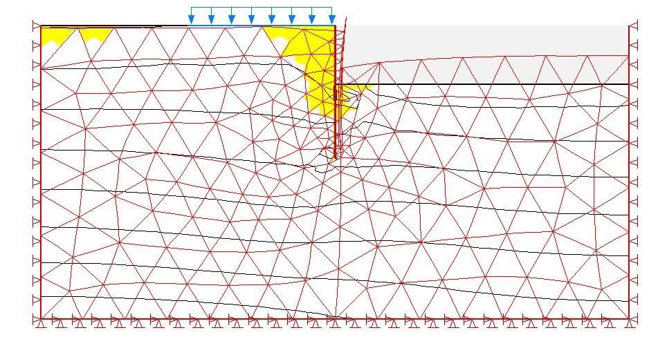
130 Figure 213: Total stress σxx for the case of a sheet pile of 9 m in sand using GeoStudio Figure 214: Total stress σyy for the case of a sheet pile of 9 m in sand using GeoStudio Figure 215: Plastic points for the case of a sheet pile of 9 m in sand using GeoStudio 129
131 2.5.6 Sand 1 st case (9 m) comparison The values obtained by SheetPile2. and by the Classic Method (that provides only the bending moment) can be considered conservative and useful for a preliminary evaluation of the parameters, whereas the FEM solutions can be chosen as more coherent with the real behavior of the soil-structure system. Regarding the bending moment obtained with the Classic Method (see chapter 2.5.2): as the minimum required length to have equilibrium is 7 m, the trend of the bending moment is taken into account only within this length and not for the remaining part of the sheet pile (Figure 217). Displacement y Plaxis SheetPile2. GeoStudio -1 x Figure 216: Displacement of a sheet pile of 9 m in sand using Plaxis, SheetPile2., GeoStudio Bending Moment y Plaxis SheetPile2. GeoStudio ClassicMethod M(y) [knm] -1 Figure 217: Bending moment of a sheet pile of 9 m in sand using Plaxis, SheetPile2., Geostudio, the Classic Method 13
132 Shear Force y T(y) [kn] Plaxis SheetPile2. GeoStudio Figure 218: Shear force of a sheet pile of 9 m in sand using Plaxis, SheetPile2., Geostudio Table 17: Maximum and minimum values of the displacement, bending moment, shear force in the sheet pile of 9 m in sand using Plaxis, SheetPile2., GeoStudio and the Classic method, absolute difference DISPLACEMENT MAXIMUM MINIMUM Plaxis SP2. GS CM Plaxis SP2. GS CM ABS_DIFF -113% 22% - ABS_DIFF 132% -7% - BENDING MOMENT [knm] MAXIMUM MINIMUM Plaxis SP2. GS CM Plaxis SP2. GS CM 1.74E E ABS_DIFF ABS_DIFF -54% 9% -69% SHEAR FORCE [kn] MAXIMUM MINIMUM Plaxis SP2. GS CM Plaxis SP2. GS CM ABS_DIFF -23% 17% - ABS_DIFF -112% 2% Classic Method Sand 2 nd case (12 m) results The only parameter that has been changed from the 1st case is the length of the sheet pile L, from L = 9 m into L = 12 m. The other parameters are the same as chapter The results are exposed in the following graphics. As the minimum required length to have equilibrium is 7 m, the trend of the bending moment is taken into account only within this length and not for the remaining part of the sheet pile (Figure 221) 131
133 Vertical Stress σv [kpa] z σv.emb σv.exc Figure 219: Vertical stress along a sheet pile of 12 m in sand using the Classic Method Horizontal Stress σh [kpa] z σh.a σh.p Figure 22: Horizontal stress along a sheet pile of 12 m in sand using the Classic Method Bending Moment M(z) [knm] z Bending Moment Figure 221: Bending moment of a sheet pile of 12 m in sand using the Classic Method 132
134 Shear Force T(z) [kn] z Sum(PA) Sum(PP) Equilibrum of Shear Force Figure 222: Shear force of a sheet pile of 12 m in sand using the Classic Method SheetPile2. Sand 2 nd case (12 m) results The only parameter that has been changed from the 1st case is the length of the sheet pile L, from L = 9 m into L = 12 m. The other parameters are the same as chapter The results are exposed in the following graphics. Table 18: Maximum and minimum values of the displacement in the sheet pile of 7.5 m and in the sheet pile of 12 m in sand using SheetPile2., absolute difference DISPLACEMENT MAXIMUM MINIMUM SP2.-7.5m SP2.-12m SP2.-7.5m SP2.-12m ABS DIFF 78% ABS DIFF 113% z Displacement x(z) Displacement Figure 223: Displacement of a sheet pile of 12 m in sand using SheetPile2. 133
135 z Angle of rotation θ(z) [rad] Angle of rotation Figure 224: Angle of rotation of a sheet pile of 12 m in sand using SheetPile z Bending Moment M(z) [knm] Bending Moment Figure 225: Bending moment of a sheet pile of 12 m in sand using SheetPile2. z Shear Force -14 T(z) [kn] Shear Force Figure 226: Shear force of a sheet pile of 12 m in sand using SheetPile2. 134
![z -4-6 -8-1 -12-14 Reaction -2-2 2 4 6 8 R(z) [kn] Reaction Figure 227: Reaction of a sheet pile of 12 m in sand using SheetPile2. 2.5.](/docs-images/82/86583395/images/136-0.jpg "9 Plaxis Sand 2 nd case (12 m) results Figure 228: Model for the case of a sheet pile of 12 m in sand using Plaxis, particular of the interface The only parameter that has been changed from the 1st")
136 z Reaction R(z) [kn] Reaction Figure 227: Reaction of a sheet pile of 12 m in sand using SheetPile Plaxis Sand 2 nd case (12 m) results Figure 228: Model for the case of a sheet pile of 12 m in sand using Plaxis, particular of the interface The only parameter that has been changed from the 1st case is the length of the sheet pile L, from L = 9 m into L = 12 m. The other parameters are the same as chapter The generated mesh (Figure 2) is a fine element distribution. The results are illustrated in the following screenshots. 135

137 Figure 229: The mesh: fine with tri-6 elements Figure 23: Deformed mesh for the case of a sheet pile of 12 m in sand using Plaxis Figure 231: Displacement ux of a sheet pile of 12 m in sand using Plaxis 136
138 Figure 232: Bending moment of a sheet pile of 12 m in sand using Plaxis Figure 233: Shear force of a sheet pile of 12 m in sand using Plaxis Figure 234: Total displacement u for the case of a sheet pile of 12 m in sand using Plaxis 137

139 Figure 235: Total stress σxx for the case of a sheet pile of 12 m in sand using Plaxis Figure 236: Total stress σyy for the case of a sheet pile of 12 m in sand using Plaxis 138
 results The only parameter that has been changed from previous chapter is the parameter Ri of the interface: it has been changed from Ri =.")
.")
140 Figure 237: Total stress σxy for the case of a sheet pile of 12 m in sand using Plaxis Figure 238: Plastic points for the case of a sheet pile of 9 m in sand using Plaxis Plaxis No Interface Sand 2 nd case (12 m) results The only parameter that has been changed from previous chapter is the parameter Ri of the interface: it has been changed from Ri =.8 into Ri = 1 ( rigid ), this new condition simulates the lack of the interface between soil and structure. The other parameters are the same as chapter The solutions with coarse and fine mesh are quite the same, whereas the model with fine mesh but with no interface differs from the previous solutions and provides lower displacement (Figure 241). Figure 239: The mesh: coarse with tri-15 elements used at the beginning for the choice of the sheet pile s length 139

141 Figure 24: The mesh: fine with tri-6 elements with no interface (Ri=1) Displacement y Coarse_Mesh_Tri15 Fine_Mesh_Tri6 Fine_Mesh_Tri6_NI -14 x Figure 241: Displacement of a sheet pile of 12 m in sand using Plaxis with: coarse mesh and tri-15 elements, fine mesh and tri-6 elements, fine mesh and tri-6 elements with no interface Table 19: Maximum and minimum values of the displacement in the sheet pile of 12 m in sand using Plaxis with: coarse mesh and tri-15 elements, fine mesh and tri-6 elements, fine mesh and tri-6 elements with no interface, absolute difference DISPLACEMENT MAXIMUM MINIMUM COARSE FINE NI COARSE FINE NI ABS_DIFF -3% 9% ABS_DIFF 1% 1% Sand 2 st case (12 m) comparison As for the 1 st case the values obtained with SheetPile2. and with the Classic Method can be considered useful to estimate the order of magnitude of the solution whereas 14
142 the FEM solutions can be chosen as more coherent with the real behavior of the soilstructure system. The difference between Plaxis and SheetPile2. decreases by 2% (Table 17, Table 2) by increasing the length of the sheet pile. y Displacement x Plaxis SheetPile2. PlaxisNI Figure 242: Displacement of a sheet pile of 12 m in sand using Plaxis, SheetPile2., Plaxis with no interface y Bending Moment M(y) [knm] Plaxis SheetPile2. PlaxisNI ClassicMethod Figure 243: Bending moment of a sheet pile of 9 m in sand using Plaxis, SheetPile2., Plaxis with no interface, the Classic Method 141
143 y Shear Force T(y) [kn] Plaxis SheetPile2. PlaxisNI Figure 244: Shear force of a sheet pile of 9 m in sand using Plaxis, SheetPile2., Plaxis with no interface Table 2: Maximum and minimum values of the displacement, bending moment, shear force in the sheet pile of 9 m in sand using Plaxis, SheetPile2., Plaxis with no interface and the Classic method, absolute difference DISPLACEMENT MAXIMUM MINIMUM Plaxis SP2. PlaxisNI CM Plaxis SP2. PlaxisNI CM ABS_DIFF -9% 12% - ABS_DIFF 77% 9% - BENDING MOMENT [knm] MAXIMUM MINIMUM Plaxis SP2. PlaxisNI CM Plaxis SP2. PlaxisNI CM ABS_DIFF - -52% - ABS_DIFF -58% 7% -58% SHEAR FORCE [kn] MAXIMUM MINIMUM Plaxis SP2. PlaxisNI CM Plaxis SP2. PlaxisNI CM ABS_DIFF -16% 3% - ABS_DIFF -34% 16% Overview of the results Clay Introduction: searching for the length to compare As for the sheet pile embedded in the granular soil, also for the case of cohesive soil it is necessary to find the suitable length that could be compared in each solution. The Classic Method gives a solution already with 8.5 m, but as said before, because of its simplicity, this method is just considered a comparison solution. The minimum 142
144 value for Sheetpile2. is 1 m, but the displacement is 33.4 cm. The minimum value for Plaxis is 8.5 m, but the displacement is cm (peak value). Plaxis provides an acceptable solution (6.811 cm) with a 12 m length sheet pile (by an increment of 1 m length the displacement decreases by 2%), but a stable solution is reached with 14 m (6.572 cm). Using a 15 m length sheet pile the performance worsens. As for the solution in the sandy soil two different comparison lengths for the sheet pile has been chosen: the first one is close to instability (1 m), the second one widely ensures the equilibrium (14 m). The other solution (for both 1 m and 14 m) has been made by using Plaxis but in this case the mesh has been set fine (around 6 elements and Ie = 2 m) keeping a 6-nodes triangle element, the value of Ri has been changed from Ri =.8 into Ri = 1 ( rigid ): this situation simulates the lack of the interface (only soil and plate) z Displacement x(z) L=8.5 L=9.5 L=1 L=11 L=12 L=13 L=14 L=15 Figure 245: Horizontal displacement of the sheet pile varying its length Table 21: Maximum and minimum values of the displacement of the sheet pile varying its length, absolute and relative difference of displacement between sheet piles with different lengths DISPLACEMENT MAXIMUM L = 8.5 L = 9.5 L = 1 L = 11 L = 12 L = 13 L = 14 L = ABS_DIFF 61% 71% 8% 82% 82% 83% 82% REL_DIFF 61% 27% 31% 8% 2% 1% -2% MINIMUM L = 8.5 L = 9.5 L = 1 L = 11 L = 12 L = 13 L = 14 L = ABS_DIFF 174% 223% 276% 289% 291% 287% 276% REL_DIFF 174% -66% -43% -7% -1% 2% 6% 143
145 2.6.2 Classic Method Clay - 1 st case (1 m) results Table 22: Parameters required in the Classic Method CLAY SP H γ φ c q dex L [kn/m 3 ] [ ] [kpa] [kn/m] Where H is thickness of the layer, γ the self-weight of sand, φ the angle of friction of sand, c the cohesion of sand, q is the load, dex the excavation, L the final length that is required for equilibrium. The results are exposed in the following graphics. As the minimum required length to have equilibrium is 8.5 m, the trend of the bending moment is taken into account only within this length and not for the remaining part of the sheet pile (Figure 248). Vertical Stress σv [kpa] z σv.emb σv.exc Figure 246: Vertical stress along a sheet pile of 1 m in clay using the Classic Method 144
146 Horizontal Stress σh [kpa] z σh.a σh.p Figure 247: Horizontal stress along a sheet pile of 1 m in clay using the Classic Method Bending Moment M(z) [knm] z Bending Moment Figure 248: Bending moment of a sheet pile of 1 m in clay using the Classic Method Shear Force T(z) [kn] z Sum(PA) Sum(PP) Equilibrum of Shear Force Figure 249: Shear force of a sheet pile of 1 m in clay using the Classic Method 145
147 2.6.3 SheetPile2. Clay - 1 st case (1 m) results Table 23: Parameters required in SheetPile2. CLAY SHEET PILE H γ φ c q dex dwl t Ep L [kn/m 3 ] [ ] [kpa] [kn/m] [kpa] x1 6 1 Where H is thickness of the layer, γ the self-weight of sand, φ the angle of friction of sand, c the cohesion of sand, q is the load, dex the excavation, dwl the depth of the groundwater level, t, Ep and L are the thickness, the elastic modulus and the length of the sheet pile respectively. The results are exposed in the following graphics. z Displacement x(z) Displacement Figure 25: Displacement of a sheet pile of 1 m in clay using SheetPile2. Table 24: Maximum and minimum values of the displacement in the sheet pile of 1 m in clay using SheetPile2. DISPLACEMENT MAXIMUM MINIMUM SP2.-1m SP2.-1m
148 -2 Angle of rotation z Angle of rotation -12 θ(z) [rad] Figure 251: Angle of rotation of a sheet pile of 1 m in clay using SheetPile2. Bending Moment z Bending Moment M(z) [knm] -12 Figure 252: Bending moment of a sheet pile of 1 m in clay using SheetPile2. Shear Force z T(z) [kn] Shear Force Figure 253: Shear force of a sheet pile of 1 m in clay using SheetPile2. 147

149 Reaction z R(z) [kn] Reaction Figure 254: Reaction of a sheet pile of 1 m in clay using SheetPile Plaxis Clay - 1 st case (1 m) results Figure 255: Model for the case of a sheet pile of 1 m in clay using Plaxis, particular of the interface The generated mesh (Figure 256) is a fine element distribution. 148

150 Figure 256: The mesh: fine with tri-6 elements These are the main characteristics of the model. The results are illustrated in the following screenshots. Table 25: Parameters required in Plaxis CLAY H γ φ c ν ψ Es q dex [kn/m 3 ] [ ] [kpa] [-] [ ] [kpa] [kn/m] x SHEET PILE IF L w EA EJ ν Ri [kn/m/m] [kn/m] [knm 2 ] [-] [-] x
151 Figure 257: Deformed mesh for the case of a sheet pile of 1 m in clay using Plaxis Figure 258: Displacement ux of a sheet pile of 1 m in clay using Plaxis Figure 259: Bending moment of a sheet pile of 1 m in clay using Plaxis 15
152 Figure 26: Shear force of a sheet pile of 1 m in clay using Plaxis Figure 261: Total displacement u for the case of a sheet pile of 1 m in clay using Plaxis Figure 262: Total stress σxx for the case of a sheet pile of 1 m in clay using Plaxis 151
153 Figure 263: Total stress σyy for the case of a sheet pile of 1 m in clay using Plaxis Figure 264: Total stress σxy for the case of a sheet pile of 1 m in clay using Plaxis Figure 265: Plastic points for the case of a sheet pile of 1 m in clay using Plaxis Plaxis No Interface Clay - 1 st case (1 m) results The only parameter that has been changed from previous chapter is the parameter Ri of the interface: it has been changed from Ri =.8 into Ri = 1 ( rigid ), this new condition simulates the lack of the interface between soil and structure. The other parameters are the same as chapter The solutions with coarse and fine mesh are quite the same, whereas the model with fine mesh but with no interface differs from the previous solutions and provides lower displacement (Figure 241). 152


154 Figure 266: The mesh: coarse with tri-15 elements used at the beginning for the choice of the sheet pile s length Figure 267: The mesh: fine with tri-6 elements with no interface (Ri=1) 153
155 Displacement y Coarse_Mesh_Tri15 Fine_Mesh_Tri6 Fine_Mesh_Tri6_NI -12 x Figure 268: Displacement of a sheet pile of 1 m in clay using Plaxis with: coarse mesh and tri-15 elements, fine mesh and tri-6 elements, fine mesh and tri-6 elements with no interface Table 26: Maximum and minimum values of the displacement in the sheet pile of 1 m in clay using Plaxis with: coarse mesh and tri-15 elements, fine mesh and tri-6 elements, fine mesh and tri-6 elements with no interface, absolute difference DISPLACEMENT MAXIMUM MINIMUM COARSE FINE NI COARSE FINE NI ABS_DIFF 5% 13% ABS_DIFF -5% -5% Clay 1 st case (1 m) comparison As for the solution with sand, the values obtained with SheetPile2. and with the Classic Method (as the minimum required length to have equilibrium is 8.5 m, the trend of the bending moment is taken into account only within this length and not for the remaining part of the sheet pile, Figure 27) can be considered adequate for a first approach to the problem whereas the FEM solutions can be chosen as more coherent with the real behavior of the soil-structure system. The latter behaves rigidly with small (Plaxis) or with almost no (SheetPile2.) curvature (Figure 269) because the sheet pile is short. 154
156 Displacement y Plaxis SheetPile2. PlaxisNI -12 x Figure 269: Displacement of a sheet pile of 1 m in clay using Plaxis, SheetPile2., Plaxis with no interface Bending Moment y Plaxis SheetPile2. PlaxisNI ClassicMethod M(y) [knm] -12 Figure 27: Bending moment of a sheet pile of 1 m in clay using Plaxis, SheetPile2., Plaxis with no interface, the Classic Method 155
157 Shear Force y T(y) [kn] Plaxis SheetPile2. PlaxisNI Figure 271: Shear force of a sheet pile of 1 m in clay using Plaxis, SheetPile2., Plaxis with no interface Table 27: Maximum and minimum values of the displacement, bending moment, shear force in the sheet pile of 1 m in clay using Plaxis, SheetPile2., Plaxis with no interface and the Classic method, absolute difference DISPLACEMENT MAXIMUM MINIMUM Plaxis SP2. PlaxisNI CM Plaxis SP2. PlaxisNI CM ABS_DIFF 74% 9% - ABS_DIFF 12% -1% - BENDING MOMENT [knm] MAXIMUM MINIMUM Plaxis SP2. PlaxisNI CM Plaxis SP2. PlaxisNI CM -4.3E E ABS_DIFF 1% 14% 1% ABS_DIFF 21% 4% 13% SHEAR FORCE [kn] MAXIMUM MINIMUM Plaxis SP2. PlaxisNI CM Plaxis SP2. PlaxisNI CM ABS_DIFF 23% 4% - ABS_DIFF 14% 3% Classic Method Clay - 2 st case (14 m) results The only parameter that has been changed from the 1st case is the length of the sheet pile L, from L = 1 m into L = 14 m. The other parameters are the same as chapter The results are exposed in the following graphics. As the minimum required length to have equilibrium is 8.5 m, the trend of the bending moment is taken into 156
158 account only within this length and not for the remaining part of the sheet pile (Figure 274). Vertical Stress σv [kpa] z σv.emb σv.exc Figure 272: Vertical stress along a sheet pile of 14 m in clay using the Classic Method Horizontal Stress σh [kpa] z σh.a σh.p Figure 273: Horizontal stress along a sheet pile of 14 m in clay using the Classic Method 157
159 Bending Moment M(z) [knm] z Bending Moment Figure 274: Bending moment of a sheet pile of 14 m in clay using the Classic Method Shear Force T(z) [kn] z Sum(PA) Sum(PP) Equilibrum of Shear Force Figure 275: Shear force of a sheet pile of 14 m in clay using the Classic Method SheetPile2. Clay - 2 st case (14 m) results The only parameter that has been changed from the 1st case is the length of the sheet pile L, from L = 1 m into L = 14 m. The other parameters are the same as chapter The results are exposed in the following graphics. Table 28: Maximum and minimum values of the displacement in the sheet pile 1 m and in the sheet pile of 14 m in clay using SheetPile2., absolute difference DISPLACEMENT MAXIMUM MINIMUM SP2.-1m SP2.-14m SP2.-1m SP2.-14m ABS_DIFF 83% ABS_DIFF 114% 158
160 z Displacement x(z) Displacement Figure 276: Displacement of a sheet pile of 14 m in clay using SheetPile z Angle of rotation θ(z) [rad] Angle of rotation Figure 277: Angle of rotation of a sheet pile of 14 m in clay using SheetPile z Bending Moment M(z) [knm] Bending Moment Figure 278: Bending moment of a sheet pile of 14 m in clay using SheetPile2. 159
161 z Shear Force T(z) [kn] Shear Force Figure 279: Shear force of a sheet pile of 14 m in clay using SheetPile2. z Reaction R(z) [kn] Reaction Figure 28: Reaction of a sheet pile of 14 m in clay using SheetPile2. 16


162 2.6.9 Plaxis Clay - 2 st case (14 m) results Figure 281: Model for the case of a sheet pile of 14 m in clay using Plaxis, particular of the interface The only parameter that has been changed from the 1st case is the length of the sheet pile L, from L = 1 m into L = 14 m. The other parameters are the same as chapter The generated mesh (Figure 282) is a fine element distribution. The results are illustrated in the following screenshots. Figure 282: The mesh: fine with tri-6 elements 161
163 Figure 283: Deformed mesh for the case of a sheet pile of 14 m in clay using Plaxis Figure 284: Displacement ux of a sheet pile of 14 m in clay using Plaxis Figure 285: Bending moment of a sheet pile of 14 m in clay using Plaxis 162
164 Figure 286: Shear force of a sheet pile of 14 m in clay using Plaxis Figure 287: Total displacement u for the case of a sheet pile of 14 m in clay using Plaxis Figure 288: Total stress σxx for the case of a sheet pile of 14 m in clay using Plaxis 163
165 Figure 289: Total stress σyy for the case of a sheet pile of 14 m in clay using Plaxis Figure 29: Total stress σxy for the case of a sheet pile of 14 m in clay using Plaxis Figure 291: Plastic points for the case of a sheet pile of 14 m in clay using Plaxis 164
, this new condition simulates the lack of the interface between soil and structure. The other parameters are the same as chapter 2.6.9.")
.")
166 2.6.1 Plaxis No Interface Clay - 2 st case (14 m) results The only parameter that has been changed from previous chapter is the parameter Ri of the interface: it has been changed from Ri =.8 into Ri = 1 ( rigid ), this new condition simulates the lack of the interface between soil and structure. The other parameters are the same as chapter As for the previous cases the solutions with coarse and fine mesh are quite the same, whereas the model with fine mesh but with no interface differs from the previous solutions and provides lower displacement (Figure 294). Figure 292: The mesh: coarse with tri-15 elements used at the beginning for the choice of the sheet pile s length Figure 293: The mesh: fine with tri-6 elements with no interface (Ri=1) 165
167 Displacement y Coarse_Mesh_Tri15 Fine_Mesh_Tri6 Fine_Mesh_Tri6_NI x Figure 294: Displacement of a sheet pile of 14 m in clay using Plaxis with: coarse mesh and tri-15 elements, fine mesh and tri-6 elements, fine mesh and tri-6 elements with no interface Table 29: Maximum and minimum values of the displacement in the sheet pile of 14 m in clay using Plaxis with: coarse mesh and tri-15 elements, fine mesh and tri-6 elements, fine mesh and tri-6 elements with no interface, absolute difference DISPLACEMENT MAXIMUM MINIMUM COARSE FINE NI COARSE FINE NI ABS_DIFF 1% 12% ABS_DIFF -1% -3% Clay 2 st case (14 m) comparison The comparison replies the evaluations exposed in the previous cases and can be assumed as a general description of the phenomenon: the solutions achieved with SheetPile2. and with the Classic Method (as the minimum required length to have equilibrium is 8.5 m, the trend of the bending moment is taken into account only within this length and not for the remaining part of the sheet pile, Figure 296) are more conservative than the ones obtained with Plaxis which; the latter better simulate the real behavior of the sheet pile and of the soil. By increasing the length of the sheet pile, the difference between Plaxis and SheetPile2. decreases by 6% (Table 27, Table 3): much more than the case of the sheet pile in sand. For this length of the sheet pile (14 m), the maximum displacement obtained with Plaxis differs only by 11% from the one of SheetPile
168 y Displacement x Plaxis SheetPile2. PlaxisNI Figure 295: Displacement of a sheet pile of 14 m in clay using Plaxis, SheetPile2., Plaxis with no interface y Bending Moment M(y) [knm] Plaxis SheetPile2. PlaxisNI ClassicMethod Figure 296: Bending moment of a sheet pile of 14 m in clay using Plaxis, SheetPile2., Plaxis with no interface, the Classic Method y Shear Force T(y) [kn] Plaxis SheetPile2. PlaxisNI Figure 297: Shear force of a sheet pile of 14 m in clay using Plaxis, SheetPile2., Plaxis with no interface 167
169 Table 3: Maximum and minimum values of the displacement, bending moment, shear force in the sheet pile of 14 m in clay using Plaxis, SheetPile2., Plaxis with no interface and the Classic method, absolute difference DISPLACEMENT MAXIMUM MINIMUM Plaxis SP2. PlaxisNI CM Plaxis SP2. PlaxisNI CM ABS_DIFF 11% 1% - ABS_DIFF 86% -2% - BENDING MOMENT [knm] MAXIMUM MINIMUM Plaxis SP2. PlaxisNI CM Plaxis SP2. PlaxisNI CM ABS_DIFF 1% -69% 1% ABS_DIFF -6% 4% 15% SHEAR FORCE [kn] MAXIMUM MINIMUM Plaxis SP2. PlaxisNI CM Plaxis SP2. PlaxisNI CM ABS_DIFF -31% % - ABS_DIFF -85% -9% - 168
170 3 Conclusions In this report, regarding the horizontal structures, the analytical methods of Winkler and Pasternak have been exposed, pointing out the equations that describe the theories (chapters 1.1.1, 1.1.2, 1.2.1, 1.2.2). The formulae have been implemented in a spreadsheet and applied to soil with absolutely generic characteristics; then the results were graphically shown (chapters 1.1.3,, 1.2.2). Applications of Pasternak s theory have been highlighted (chapter 1.2). The numerical solution obtained with FEM program GeoStudio has been illustrated and compared to the analytical solutions (chapter ). Description of the constitutive material models has been made; results obtained by elastic and elastic-plastic analysis applied to the previous issue using the FEM program Midas GTS have been exposed (chapter 1.3). In the following graphics and table a comparison between all these approaches is shown, highlighting the topic values (Figure 298, Figure 299, Figure 3, Table 31). One can see that the Winkler s approach is the most conservative, and is matched by the solution of Pasternak adopting S = 1 kn (the membrane doesn t work), see Figure 298. The solution of Pasternak adopting S calculated by the formula suggested in chapter m provides lower displacement than the one of Winkler, and is closer to the solution by FEM. Results by FEM programs GeoStudio (elastic) and Midas (elastic and elastic-plastic) match, with no differences between elastic and elastic-plastic due to the limited value of load applied to the foundations. FEM programs give the most accurate solution to the problem considering the theoretical feedback that is compulsory in their implementation, but the simplified theories of Winkler and Pasternak can be successfully used in order to obtain an approximate solution to the problem and general information regarding the order of magnitude of the results. The implementation of the analytical methods of Winkler and Pasternak is efficient because one obtains an immediate evaluation of the parameters changing the input data. The solution with the spreadsheet is versatile because one can analyze different load conditions modifying the border conditions of the equation that describes the problem. 169
171 Displacement.2 w(x) x Winkler_Analytical GeoStudio_Elastic Pasternak S calc Pasternak S=1 Midas_Elastic Midas_EP Figure 298: Displacement obtained by varying the approach to the issue M(x) [knm] Bending Moment x Winkler_Analytical GeoStudio_Elastic Pasternak S calc Paternak S=1 Midas_Elastic Midas_EP Figure 299: Bending moment obtained by varying the approach to the issue T(x) [kn] Shear Force x Winkler_Analytical GeoStudio_Elastic Pasternak S calc Pasternak S=1 Midas_Elastic Midas_EP Figure 3: Shear force obtained by varying the approach to the issue 17
172 Table 31: Maximum and minimum values of the displacement, bending moment, shear force of the loaded beam varying the calculation approach (Winkle implemented in a spreadsheet, GeoStudio, Pasternak implemented in a spreadsheet with S calculated by the formula suggested in the chapter 1.2.1, Pasternak implemented in a spreadsheet with S=1 kn, Midas linear elastic, Midas elastic-plastic), absolute difference DISPLACEMENT MAXIMUM Winkler GeoStudio_LE Pasternak S calc Pasternak S=1 Midas_LE Midas_EP ABS_DIFF 36% 28% 1% 37% 37% MINIMUM Winkler GeoStudio_LE Pasternak S calc Pasternak S=1 Midas_LE Midas_EP ABS_DIFF 37% 29% % 39% 39% BENDING MOMENT [knm] MAXIMUM Winkler GeoStudio_LE Pasternak S calc Pasternak S=1 Midas_LE Midas_EP ABS_DIFF 59% 61% 16% 59% 59% MINIMUM Winkler GeoStudio_LE Pasternak S calc Pasternak S=1 Midas_LE Midas_EP ABS_DIFF -21% -223% 8% -236% -236% SHEAR FORCE [kn] MAXIMUM Winkler GeoStudio_LE Pasternak S calc Pasternak S=1 Midas_LE Midas_EP ABS_DIFF -158% -113% -2% -137% -137% MINIMUM Winkler GeoStudio_LE Pasternak S calc Pasternak S=1 Midas_LE Midas_EP ABS_DIFF 34% 29% 1% 39% 39% 171
173 Regarding the vertical structures, the simplified limit equilibrium method has been exposed (chapter 2.2) and application of it on sheet pile embedded in either sandy or clay soil has been implemented (chapters 2.5, 2.6). The theory of the dependent pressure method has been illustrated (chapter 2.3) and the calculation with the relative program has been made, considering the same set of conditions (sand or clay, length of the sheet pile) used in the previous approach (chapters 2.5, 2.6). The FEM programs Plaxis and GeoStudio have been described (chapter 2.4), and the obtained results on the set of conditions previously enounced have been shown (chapters 2.5, 2.6). Comparison between all these approaches has been made, preliminarily varying the length of the sheet pile (using Plaxis) and afterwards choosing the comparison lengths: firstly, an embedment that widely ensures the equilibrium, secondly, a solution close to instability (chapters 2.5, 2.6). In the following graphics the topic results are summarized. In Figure 31 one can see the behavior of the sheet pile varying the embedment length from an instable condition to a stable one, for sandy and clay soil. In Figure 32 one can see the case of a sheet pile of 9 m embedded in sand studied by the support of the Classic Method, SheetPile2., GeoStudio and Plaxis. The FEM programs ensure the most accurate results, but SheetPile2. and the Classic Method (which can only estimate the bending moment along the sheet pile) could give an approximate evaluation of the solution which can be useful for preliminary studies on the issue. In Figure 33 the behavior of a sheet pile of 1 m (close to instability) and that of a 14 m one (stable situation), both embedded in clay and with varying mesh coarseness, element types and both first considering then ignoring the interface element, is shown (using Plaxis). The accuracy of the solution changes according to the choice of the element and the coarseness, but not significantly: of course it depends on the precision required by the analysis. The lack of the interface element changes the solution providing lower displacement to the sheet pile, whereas the use of the interface element provides conservative results. 172
174 z Displacement x(z) L=8.5 L=9 L=1 L=11 L=12 L=13 L= z Displacement x(z) L=8.5 L=9.5 L=1 L=11 L=12 L=13 L=14 L=15 Figure 31: Searching for the length to compare by using Plaxis, sandy soil and clay soil 173
175 Displacement y Plaxis SheetPile2. GeoStudio -1 x Bending Moment y Plaxis SheetPile2. GeoStudio ClassicMethod M(y) [knm] -1 Shear Force y T(y) [kn] Plaxis SheetPile2. GeoStudio Figure 32: Displacement, bending moment, shear force of a sheet pile of 9 m in sand varying the calculation approach (Plaxis, SheetPile2., GeoStudio, Classic Method) 174
176 Displacement y Coarse_Mesh_Tri15 Fine_Mesh_Tri6 Fine_Mesh_Tri6_NI -12 x y Displacement x Coarse_Mesh_Tri15 Fine_Mesh_Tri6 Fine_Mesh_Tri6_NI Figure 33: Displacement of a sheet pile of 1 m and of 14 m in clay using Plaxis varying the mesh coarseness, the element type and considering or not the interface element Some further applications or studies can be suggested and summarized as follows: Analyses of the response of the foundation studied in chapter 1.3, modelized with plate elements instead of the beam element, either with an elastic or elastic-plastic constitutive model: in this way the focus would be on the behavior of the foundations, simulating more accurately the trend of compression and tensile stress within the concrete Validation of the Pasternak 3D model illustrated in the chapter (Figure 34) by comparison with real data from loaded membrane applied on gravel columns To verify if a further improvement of SheetPile2. program is achievable in order to gain more accuracy in terms of displacement and stress parameters 175

177 Further studies on the interface element, characteristic which highly influences both the response of the sheet pile in excavation and under load, and the soil-structure interaction considered in other application fields. Figure 34: Behavior of a loaded membrane applied on gravel columns 176
Numerical and Theoretical Study of Plate Load Test to Define Coefficient of Subgrade Reaction
 Journal of Geotechnical and Transportation Engineering Volume 1 Issue 2 Numerical and Theoretical Study of Plate Load Test to Define Coefficient of Subgrade Reaction Naeini and Taherabadi Received 9/28/2015
DYNAMIC ANALYSIS OF PILES IN SAND BASED ON SOIL-PILE INTERACTION
 October 1-17,, Beijing, China DYNAMIC ANALYSIS OF PILES IN SAND BASED ON SOIL-PILE INTERACTION Mohammad M. Ahmadi 1 and Mahdi Ehsani 1 Assistant Professor, Dept. of Civil Engineering, Geotechnical Group,
FINITE GRID SOLUTION FOR NON-RECTANGULAR PLATES
 th International Conference on Earthquake Geotechnical Engineering June 5-8, 7 Paper No. 11 FINITE GRID SOLUTION FOR NON-RECTANGULAR PLATES A.Halim KARAŞĐN 1, Polat GÜLKAN ABSTRACT Plates on elastic foundations
Finite Element Method in Geotechnical Engineering
 Finite Element Method in Geotechnical Engineering Short Course on + Dynamics Boulder, Colorado January 5-8, 2004 Stein Sture Professor of Civil Engineering University of Colorado at Boulder Contents Steps
PILE-SUPPORTED RAFT FOUNDATION SYSTEM
 PILE-SUPPORTED RAFT FOUNDATION SYSTEM Emre Biringen, Bechtel Power Corporation, Frederick, Maryland, USA Mohab Sabry, Bechtel Power Corporation, Frederick, Maryland, USA Over the past decades, there has
Finite Element Investigation of the Interaction between a Pile and a Soft Soil focussing on Negative Skin Friction
 NGM 2016 Reykjavik Proceedings of the 17 th Nordic Geotechnical Meeting Challenges in Nordic Geotechnic 25 th 28 th of May Finite Element Investigation of the Interaction between a Pile and a Soft Soil
Analysis of CMC-Supported Embankments Considering Soil Arching
 Analysis of CMC-Supported Embankments Considering Soil Arching Balaka Ghosh 1, Behzad Fatahi 2, Hadi Khabbaz 3, and A. H. M. Kamruzzaman 4 1 PhD Candidate, School of Civil and Environmental Engineering,
BENCHMARK LINEAR FINITE ELEMENT ANALYSIS OF LATERALLY LOADED SINGLE PILE USING OPENSEES & COMPARISON WITH ANALYTICAL SOLUTION
 BENCHMARK LINEAR FINITE ELEMENT ANALYSIS OF LATERALLY LOADED SINGLE PILE USING OPENSEES & COMPARISON WITH ANALYTICAL SOLUTION Ahmed Elgamal and Jinchi Lu October 07 Introduction In this study: I) The response
TC211 Workshop CALIBRATION OF RIGID INCLUSION PARAMETERS BASED ON. Jérôme Racinais. September 15, 2015 PRESSUMETER TEST RESULTS
 Jérôme Racinais September 15, 215 TC211 Workshop CALIBRATION OF RIGID INCLUSION PARAMETERS BASED ON PRESSUMETER TEST RESULTS Table of contents 1. Reminder about pressuremeter tests 2. General behaviour
Seismic Response Analysis of Structure Supported by Piles Subjected to Very Large Earthquake Based on 3D-FEM
 Seismic Response Analysis of Structure Supported by Piles Subjected to Very Large Earthquake Based on 3D-FEM *Hisatoshi Kashiwa 1) and Yuji Miyamoto 2) 1), 2) Dept. of Architectural Engineering Division
Using MATLAB and. Abaqus. Finite Element Analysis. Introduction to. Amar Khennane. Taylor & Francis Croup. Taylor & Francis Croup,
 Introduction to Finite Element Analysis Using MATLAB and Abaqus Amar Khennane Taylor & Francis Croup Boca Raton London New York CRC Press is an imprint of the Taylor & Francis Croup, an informa business
Finite Element analysis of Laterally Loaded Piles on Sloping Ground
 Indian Geotechnical Journal, 41(3), 2011, 155-161 Technical Note Finite Element analysis of Laterally Loaded Piles on Sloping Ground K. Muthukkumaran 1 and N. Almas Begum 2 Key words Lateral load, finite
Dynamics Manual. Version 7
 Dynamics Manual Version 7 DYNAMICS MANUAL TABLE OF CONTENTS 1 Introduction...1-1 1.1 About this manual...1-1 2 Tutorial...2-1 2.1 Dynamic analysis of a generator on an elastic foundation...2-1 2.1.1 Input...2-1
CHAPTER 8 ANALYSES OF THE LATERAL LOAD TESTS AT THE ROUTE 351 BRIDGE
 CHAPTER ANALYSES OF THE LATERAL LOAD TESTS AT THE ROUTE 351 BRIDGE.1 INTRODUCTION An important objective of this research is to determine whether accurate analyses of the lateral load-deflection behavior
CRITERIA FOR SELECTION OF FEM MODELS.
 CRITERIA FOR SELECTION OF FEM MODELS. Prof. P. C.Vasani,Applied Mechanics Department, L. D. College of Engineering,Ahmedabad- 380015 Ph.(079) 7486320 [R] E-mail:pcv-im@eth.net 1. Criteria for Convergence.
PLAXIS 3D FOUNDATION Validation Manual. version 1.5
 PLAXIS 3D FOUNDATION Validation Manual version 1.5 TABLE OF CONTENTS TABLE OF CONTENTS 1 Introduction...1-1 2 Soil model problems with known theoretical solutions...2-1 2.1 Bi-axial test with linear elastic
Gapping effects on the lateral stiffness of piles in cohesive soil
 Gapping effects on the lateral stiffness of piles in cohesive soil Satyawan Pranjoto Engineering Geology, Auckland, New Zealand. M. J. Pender Department of Civil and Environmental Engineering, University
PURE BENDING. If a simply supported beam carries two point loads of 10 kn as shown in the following figure, pure bending occurs at segment BC.
 BENDING STRESS The effect of a bending moment applied to a cross-section of a beam is to induce a state of stress across that section. These stresses are known as bending stresses and they act normally
1 Introduction. Abstract
 Abstract This paper presents a three-dimensional numerical model for analysing via finite element method (FEM) the mechanized tunneling in urban areas. The numerical model is meant to represent the typical
NUMERICAL ANALYSIS OF A PILE SUBJECTED TO LATERAL LOADS
 IGC 009, Guntur, INDIA NUMERICAL ANALYSIS OF A PILE SUBJECTED TO LATERAL LOADS Mohammed Younus Ahmed Graduate Student, Earthquake Engineering Research Center, IIIT Hyderabad, Gachibowli, Hyderabad 3, India.
Numerical Investigation of the Effect of Recent Load History on the Behaviour of Steel Piles under Horizontal Loading
 Numerical Investigation of the Effect of Recent Load History on the Behaviour of Steel Piles under Horizontal Loading K. Abdel-Rahman Dr.-Ing., Institute of Soil Mechanics, Foundation Engineering and Waterpower
Example-3. Title. Description. Cylindrical Hole in an Infinite Mohr-Coulomb Medium
 Example-3 Title Cylindrical Hole in an Infinite Mohr-Coulomb Medium Description The problem concerns the determination of stresses and displacements for the case of a cylindrical hole in an infinite elasto-plastic
SOIL MODELS: SAFETY FACTORS AND SETTLEMENTS
 PERIODICA POLYTECHNICA SER. CIV. ENG. VOL. 48, NO. 1 2, PP. 53 63 (2004) SOIL MODELS: SAFETY FACTORS AND SETTLEMENTS Gabriella VARGA and Zoltán CZAP Geotechnical Department Budapest University of Technology
UNIVERSITY OF SASKATCHEWAN ME MECHANICS OF MATERIALS I FINAL EXAM DECEMBER 13, 2008 Professor A. Dolovich
 UNIVERSITY OF SASKATCHEWAN ME 313.3 MECHANICS OF MATERIALS I FINAL EXAM DECEMBER 13, 2008 Professor A. Dolovich A CLOSED BOOK EXAMINATION TIME: 3 HOURS For Marker s Use Only LAST NAME (printed): FIRST
Lecture 15 Strain and stress in beams
 Spring, 2019 ME 323 Mechanics of Materials Lecture 15 Strain and stress in beams Reading assignment: 6.1 6.2 News: Instructor: Prof. Marcial Gonzalez Last modified: 1/6/19 9:42:38 PM Beam theory (@ ME
FLEXIBILITY METHOD FOR INDETERMINATE FRAMES
 UNIT - I FLEXIBILITY METHOD FOR INDETERMINATE FRAMES 1. What is meant by indeterminate structures? Structures that do not satisfy the conditions of equilibrium are called indeterminate structure. These
CHAPTER 3 ANALYSIS OF BEAMS *ON ELASTIC FOUNDATION. The continuous beam type of footing system is generally
 CHAPTER 3 ANALYSIS OF BEAMS *ON ELASTIC FOUNDATION The continuous beam type of footing system is generally analysed as beam on elastic foundation. Such a structural system for the footing ensures flexural
Towards Efficient Finite Element Model Review Dr. Richard Witasse, Plaxis bv (based on the original presentation of Dr.
 Towards Efficient Finite Element Model Review Dr. Richard Witasse, Plaxis bv (based on the original presentation of Dr. Brinkgreve) Journée Technique du CFMS, 16 Mars 2011, Paris 1/32 Topics FEA in geotechnical
Soil Mechanics Prof. B.V.S. Viswanathan Department of Civil Engineering Indian Institute of Technology, Bombay Lecture 51 Earth Pressure Theories II
 Soil Mechanics Prof. B.V.S. Viswanathan Department of Civil Engineering Indian Institute of Technology, Bombay Lecture 51 Earth Pressure Theories II Welcome to lecture number two on earth pressure theories.
Single Pile Simulation and Analysis Subjected to Lateral Load
 Single Pile Simulation and Analysis Subjected to Lateral Load Jasim M Abbas Ph D Student, Department of Civil and Structural Engineering, Universiti Kebangsaan Malaysia e-mail: jasimalshamary@yahoo.com
Cubzac-les-Ponts Experimental Embankments on Soft Clay
 Cubzac-les-Ponts Experimental Embankments on Soft Clay 1 Introduction In the 197 s, a series of test embankments were constructed on soft clay at Cubzac-les-Ponts in France. These full-scale field tests
International Journal of Advanced Engineering Technology E-ISSN
 Research Article INTEGRATED FORCE METHOD FOR FIBER REINFORCED COMPOSITE PLATE BENDING PROBLEMS Doiphode G. S., Patodi S. C.* Address for Correspondence Assistant Professor, Applied Mechanics Department,
Lecture 2: Stresses in Pavements
 Lecture 2: Stresses in Pavements Stresses in Layered Systems At any point, 9 stresses exist. They are 3 normal stresses (s z, s r, s t ) and 6 shearing stresses ( t rz = t zr, t rt = t tr, and t tz = t
Analysis of Blocky Rock Slopes with Finite Element Shear Strength Reduction Analysis
 Analysis of Blocky Rock Slopes with Finite Element Shear Strength Reduction Analysis R.E. Hammah, T. Yacoub, B. Corkum & F. Wibowo Rocscience Inc., Toronto, Canada J.H. Curran Department of Civil Engineering
Numerical Modeling of Interface Between Soil and Pile to Account for Loss of Contact during Seismic Excitation
 Numerical Modeling of Interface Between Soil and Pile to Account for Loss of Contact during Seismic Excitation P. Sushma Ph D Scholar, Earthquake Engineering Research Center, IIIT Hyderabad, Gachbowli,
ENGN 2340 Final Project Report. Optimization of Mechanical Isotropy of Soft Network Material
 ENGN 2340 Final Project Report Optimization of Mechanical Isotropy of Soft Network Material Enrui Zhang 12/15/2017 1. Introduction of the Problem This project deals with the stress-strain response of a
Engineeringmanuals. Part2
 Engineeringmanuals Part2 Engineering manuals for GEO5 programs Part 2 Chapter 1-12, refer to Engineering Manual Part 1 Chapter 13. Pile Foundations Introduction... 2 Chapter 14. Analysis of vertical load-bearing
A METHOD OF LOAD INCREMENTS FOR THE DETERMINATION OF SECOND-ORDER LIMIT LOAD AND COLLAPSE SAFETY OF REINFORCED CONCRETE FRAMED STRUCTURES
 A METHOD OF LOAD INCREMENTS FOR THE DETERMINATION OF SECOND-ORDER LIMIT LOAD AND COLLAPSE SAFETY OF REINFORCED CONCRETE FRAMED STRUCTURES Konuralp Girgin (Ph.D. Thesis, Institute of Science and Technology,
FINITE ELEMENT ANALYSIS OF ARKANSAS TEST SERIES PILE #2 USING OPENSEES (WITH LPILE COMPARISON)
") FINITE ELEMENT ANALYSIS OF ARKANSAS TEST SERIES PILE #2 USING OPENSEES (WITH LPILE COMPARISON) Ahmed Elgamal and Jinchi Lu October 07 Introduction In this study, we conduct a finite element simulation
FINITE ELEMENT ANALYSIS OF ARKANSAS TEST SERIES PILE #2 USING OPENSEES (WITH LPILE COMPARISON) Ahmed Elgamal and Jinchi Lu October 07 Introduction In this study, we conduct a finite element simulation
Mechanical Behaviors of Cylindrical Retaining Structures in Ultra-deep Excavation
 Mechanical Behaviors of Cylindrical Retaining Structures in Ultra-deep Excavation Pengfei Xu Tongji University August 4, 2015 Outline Introduction Two circular excavations for anchorage foundations 3D
Verification of the Hyperbolic Soil Model by Triaxial Test Simulations
 1 Introduction Verification of the Hyperbolic Soil Model by Triaxial Test Simulations This example simulates a series of triaxial tests that can be used to verify that the Hyperbolic constitutive model
ANALYSIS OF LATERALLY LOADED FIXED HEADED SINGLE FLOATING PILE IN MULTILAYERED SOIL USING BEF APPROACH
 INDIAN GEOTECHNICAL SOCIETY, KOLKATA CHAPTER GEOTECHNICS FOR INFRASTRUCTURE DEVELOPMENT KOLKATA 11 th 12 th March 2016, Kolkata, West Bengal, India ANALYSIS OF LATERALLY LOADED FIXED HEADED SINGLE FLOATING
Chapter 5 CENTRIC TENSION OR COMPRESSION ( AXIAL LOADING )
") Chapter 5 CENTRIC TENSION OR COMPRESSION ( AXIAL LOADING ) 5.1 DEFINITION A construction member is subjected to centric (axial) tension or compression if in any cross section the single distinct stress
Chapter 5 CENTRIC TENSION OR COMPRESSION ( AXIAL LOADING ) 5.1 DEFINITION A construction member is subjected to centric (axial) tension or compression if in any cross section the single distinct stress
Chapter 12. Static Equilibrium and Elasticity
 Chapter 12 Static Equilibrium and Elasticity Static Equilibrium Equilibrium implies that the object moves with both constant velocity and constant angular velocity relative to an observer in an inertial
Dynamic Response of EPS Blocks /soil Sandwiched Wall/embankment
 Proc. of Second China-Japan Joint Symposium on Recent Development of Theory and Practice in Geotechnology, Hong Kong, China Dynamic Response of EPS Blocks /soil Sandwiched Wall/embankment J. C. Chai 1
Aim of the study Experimental determination of mechanical parameters Local buckling (wrinkling) Failure maps Optimization of sandwich panels
 Failure maps Optimization of sandwich panels") METNET Workshop October 11-12, 2009, Poznań, Poland Experimental and numerical analysis of sandwich metal panels Zbigniew Pozorski, Monika Chuda-Kowalska, Robert Studziński, Andrzej Garstecki Poznan University
METNET Workshop October 11-12, 2009, Poznań, Poland Experimental and numerical analysis of sandwich metal panels Zbigniew Pozorski, Monika Chuda-Kowalska, Robert Studziński, Andrzej Garstecki Poznan University
Advanced Structural Analysis EGF Section Properties and Bending
 Advanced Structural Analysis EGF316 3. Section Properties and Bending 3.1 Loads in beams When we analyse beams, we need to consider various types of loads acting on them, for example, axial forces, shear
2D Liquefaction Analysis for Bridge Abutment
 D Liquefaction Analysis for Bridge Abutment Tutorial by Angel Francisco Martinez Integrated Solver Optimized for the next generation 64-bit platform Finite Element Solutions for Geotechnical Engineering
PLAT DAN CANGKANG (TKS 4219)
") PLAT DAN CANGKANG (TKS 4219) SESI I: PLATES Dr.Eng. Achfas Zacoeb Dept. of Civil Engineering Brawijaya University INTRODUCTION Plates are straight, plane, two-dimensional structural components of which
PLAT DAN CANGKANG (TKS 4219) SESI I: PLATES Dr.Eng. Achfas Zacoeb Dept. of Civil Engineering Brawijaya University INTRODUCTION Plates are straight, plane, two-dimensional structural components of which
Rigid pavement design
 Rigid pavement design Lecture Notes in Transportation Systems Engineering Prof. Tom V. Mathew Contents 1 Overview 1 1.1 Modulus of sub-grade reaction.......................... 2 1.2 Relative stiffness
Structural Dynamics Lecture Eleven: Dynamic Response of MDOF Systems: (Chapter 11) By: H. Ahmadian
 By: H. Ahmadian") Structural Dynamics Lecture Eleven: Dynamic Response of MDOF Systems: (Chapter 11) By: H. Ahmadian ahmadian@iust.ac.ir Dynamic Response of MDOF Systems: Mode-Superposition Method Mode-Superposition Method:
Structural Dynamics Lecture Eleven: Dynamic Response of MDOF Systems: (Chapter 11) By: H. Ahmadian ahmadian@iust.ac.ir Dynamic Response of MDOF Systems: Mode-Superposition Method Mode-Superposition Method:
CHAPTER 5. Beam Theory
 CHPTER 5. Beam Theory SangJoon Shin School of Mechanical and erospace Engineering Seoul National University ctive eroelasticity and Rotorcraft Lab. 5. The Euler-Bernoulli assumptions One of its dimensions
Numerical Modelling of Dynamic Earth Force Transmission to Underground Structures
 Numerical Modelling of Dynamic Earth Force Transmission to Underground Structures N. Kodama Waseda Institute for Advanced Study, Waseda University, Japan K. Komiya Chiba Institute of Technology, Japan
UNIT IV FLEXIBILTY AND STIFFNESS METHOD
 SIDDHARTH GROUP OF INSTITUTIONS :: PUTTUR Siddharth Nagar, Narayanavanam Road 517583 QUESTION BANK (DESCRIPTIVE) Subject with Code : SA-II (13A01505) Year & Sem: III-B.Tech & I-Sem Course & Branch: B.Tech
Computational Simulation of Dynamic Response of Vehicle Tatra T815 and the Ground
 IOP Conference Series: Earth and Environmental Science PAPER OPEN ACCESS Computational Simulation of Dynamic Response of Vehicle Tatra T815 and the Ground To cite this article: Jozef Vlek and Veronika
ON THE FACE STABILITY OF TUNNELS IN WEAK ROCKS
 33 rd 33 Annual rd Annual General General Conference conference of the Canadian of the Canadian Society for Society Civil Engineering for Civil Engineering 33 e Congrès général annuel de la Société canadienne
Cyclic lateral response of piles in dry sand: Effect of pile slenderness
 Cyclic lateral response of piles in dry sand: Effect of pile slenderness Rafa S. 1, Rouaz I. 1,Bouaicha A. 1, Abed El Hamid A. 1 Rafa.sidali@gmail.com 1 National Center for Studies and Integrated Researches
Laboratory 4 Topic: Buckling
 Laboratory 4 Topic: Buckling Objectives: To record the load-deflection response of a clamped-clamped column. To identify, from the recorded response, the collapse load of the column. Introduction: Buckling
Determination of subgrade reaction modulus of two layered soil
 3 r d International Conference on New Developments in Soil Mechanics and Geotechnical Engineering, 28-30 June 2012, Near East University, Nicosia, North Cyprus Determination of subgrade reaction modulus
Landslide FE Stability Analysis
 Landslide FE Stability Analysis L. Kellezi Dept. of Geotechnical Engineering, GEO-Danish Geotechnical Institute, Denmark S. Allkja Altea & Geostudio 2000, Albania P. B. Hansen Dept. of Geotechnical Engineering,
Analysis of Load-Settlement Relationship for Unpaved Road Reinforced with Geogrid
 ISGSR7 First International Symposium on Geotechnical Safety & Risk Oct. 8~9, 7 Shanghai Tongji University, China Analysis of Load-Settlement Relationship for Unpaved Road Reinforced with Geogrid Y. C.
Analysis and measurements of settlement for heavy loaded rigid footing
 Analysis and measurements of settlement for heavy loaded rigid footing I. Sokoli University of Zagreb, Faculty of Civil Engineering, Ka i eva 26, 1 Zagreb, Croatia T. Ivši University of Zagreb, Faculty
Level 7 Postgraduate Diploma in Engineering Computational mechanics using finite element method
 9210-203 Level 7 Postgraduate Diploma in Engineering Computational mechanics using finite element method You should have the following for this examination one answer book No additional data is attached
Analysis of Infinitely Long Euler Bernoulli Beam on Two Parameter Elastic Foundation: Case of Point Load
 Analysis of Infinitely Long Euler Bernoulli Beam on Two Parameter Elastic Foundation: Case of Point Load Dr. Mama, Benjamin Okwudili Department of Civil Engineering, University of Nigeria, Nsukka. benjamin.mama@unn.edu.ng
Copyright. magazine. bearing capacity and modulus of subgrade reaction? Modulus of Subgrade Reaction (Ks)
") Structural Design design issues for structural engineers Correlation between Soil Bearing Capacity and Modulus of Subgrade Reaction By Apurba Tribedi Apurba Tribedi is a Senior Product Manager at Bentley.
Structural Design design issues for structural engineers Correlation between Soil Bearing Capacity and Modulus of Subgrade Reaction By Apurba Tribedi Apurba Tribedi is a Senior Product Manager at Bentley.
INFLUENCE OF SUBGRADE MODULUS AND THICKNESS ON THE BEHAVIOUR OF RAFT FOUNDATION
 INFLUENCE OF SUBGRADE MODULUS AND THICKNESS ON THE BEHAVIOUR OF RAFT FOUNDATION Ranjitha P 1, Sathyanarayanan Sridhar R 2 1 Post Graduate student, M.E. Computer Methods and applications in Structural Engineering,
If you take CT5143 instead of CT4143 then write this at the first of your answer sheets and skip problem 4 and 6.
 Delft University of Technology Faculty of Civil Engineering and Geosciences Structural Mechanics Section Write your name and study number at the top right-hand of your work. Exam CT4143 Shell Analysis
Finite Element Analysis Prof. Dr. B. N. Rao Department of Civil Engineering Indian Institute of Technology, Madras. Module - 01 Lecture - 11
 Finite Element Analysis Prof. Dr. B. N. Rao Department of Civil Engineering Indian Institute of Technology, Madras Module - 01 Lecture - 11 Last class, what we did is, we looked at a method called superposition
Discrete Analysis for Plate Bending Problems by Using Hybrid-type Penalty Method
 131 Bulletin of Research Center for Computing and Multimedia Studies, Hosei University, 21 (2008) Published online (http://hdl.handle.net/10114/1532) Discrete Analysis for Plate Bending Problems by Using
Evaluation of dynamic behavior of culverts and embankments through centrifuge model tests and a numerical analysis
 Computer Methods and Recent Advances in Geomechanics Oka, Murakami, Uzuoka & Kimoto (Eds.) 2015 Taylor & Francis Group, London, ISBN 978-1-138-00148-0 Evaluation of dynamic behavior of culverts and embankments
Hyperbolic Soil Bearing Capacity
 1 Introduction Hyperbolic Soil Bearing Capacity This example involves analyzing the bearing capacity of a round footing. The example is useful for illustrating several SIGMA/W features and procedures,
Calculation and analysis of internal force of piles excavation supporting. based on differential equation. Wei Wang
 International Conference on Energy and Environmental Protection (ICEEP 016) Calculation and analysis of internal force of piles excavation supporting based on differential equation Wei Wang School of Prospecting
AERSYS KNOWLEDGE UNIT
 -7016 1. INTRODUCTION The scope of this document is to provide a clarification and a deeper understanding of the two different ways to move the mid plane of the element out of the nodal plane. Although
Limit analysis of brick masonry shear walls with openings under later loads by rigid block modeling
 Limit analysis of brick masonry shear walls with openings under later loads by rigid block modeling F. Portioli, L. Cascini, R. Landolfo University of Naples Federico II, Italy P. Foraboschi IUAV University,
TIME-DEPENDENT BEHAVIOR OF PILE UNDER LATERAL LOAD USING THE BOUNDING SURFACE MODEL
 TIME-DEPENDENT BEHAVIOR OF PILE UNDER LATERAL LOAD USING THE BOUNDING SURFACE MODEL Qassun S. Mohammed Shafiqu and Maarib M. Ahmed Al-Sammaraey Department of Civil Engineering, Nahrain University, Iraq
Cavity Expansion Methods in Geomechanics
 Cavity Expansion Methods in Geomechanics by Hai-Sui Yu School of Civil Engineering, University of Nottingham, U. K. KLUWER ACADEMIC PUBLISHERS DORDRECHT / BOSTON / LONDON TABLE OF CONTENTS Foreword Preface
FIXED BEAMS IN BENDING
 FIXED BEAMS IN BENDING INTRODUCTION Fixed or built-in beams are commonly used in building construction because they possess high rigidity in comparison to simply supported beams. When a simply supported
Minimization Solutions for Vibrations Induced by Underground Train Circulation
 Minimization Solutions for Vibrations Induced by Underground Train Circulation Carlos Dinis da Gama 1, Gustavo Paneiro 2 1 Professor and Head, Geotechnical Center of IST, Technical University of Lisbon,
CASE STUDIES IN RAILWAY CONSTRUCTION
 MSC COURSE 2016/2017 AUTUMN SEMESTER CASE STUDIES IN RAILWAY CONSTRUCTION RAILWAY SUPERSTRUCTURE CALCULATION ZIMMERMANN-EISENMANN METHOD SZÉCHENYI ISTVÁN UNIVERSITY Zoltán MAJOR junior lecturer Conventional
Pile-clayey soil interaction analysis by boundary element method
 Journal of Rock Mechanics and Geotechnical Engineering. 12, 4 (1): 28 43 Pile-clayey soil interaction analysis by boundary element method Mohammed Y. Fattah 1, Kais T. Shlash 1, Madhat S. M. Al-Soud 2
Chapter 3 LAMINATED MODEL DERIVATION
 17 Chapter 3 LAMINATED MODEL DERIVATION 3.1 Fundamental Poisson Equation The simplest version of the frictionless laminated model was originally introduced in 1961 by Salamon, and more recently explored
GATE SOLUTIONS E N G I N E E R I N G
 GATE SOLUTIONS C I V I L E N G I N E E R I N G From (1987-018) Office : F-16, (Lower Basement), Katwaria Sarai, New Delhi-110016 Phone : 011-65064 Mobile : 81309090, 9711853908 E-mail: info@iesmasterpublications.com,
Centrifuge Shaking Table Tests and FEM Analyses of RC Pile Foundation and Underground Structure
 Centrifuge Shaking Table s and FEM Analyses of RC Pile Foundation and Underground Structure Kenji Yonezawa Obayashi Corporation, Tokyo, Japan. Takuya Anabuki Obayashi Corporation, Tokyo, Japan. Shunichi
PILE SOIL INTERACTION MOMENT AREA METHOD
 Pile IGC Soil 2009, Interaction Moment Guntur, INDIA Area Method PILE SOIL INTERACTION MOMENT AREA METHOD D.M. Dewaikar Professor, Department of Civil Engineering, IIT Bombay, Mumbai 400 076, India. E-mail:
7.4 The Elementary Beam Theory
 7.4 The Elementary Beam Theory In this section, problems involving long and slender beams are addressed. s with pressure vessels, the geometry of the beam, and the specific type of loading which will be
Discrete Element Modelling of a Reinforced Concrete Structure
 Discrete Element Modelling of a Reinforced Concrete Structure S. Hentz, L. Daudeville, F.-V. Donzé Laboratoire Sols, Solides, Structures, Domaine Universitaire, BP 38041 Grenoble Cedex 9 France sebastian.hentz@inpg.fr
CHAPTER THREE SYMMETRIC BENDING OF CIRCLE PLATES
 CHAPTER THREE SYMMETRIC BENDING OF CIRCLE PLATES * Governing equations in beam and plate bending ** Solution by superposition 1.1 From Beam Bending to Plate Bending 1.2 Governing Equations For Symmetric
CALCULATION OF A SHEET PILE WALL RELIABILITY INDEX IN ULTIMATE AND SERVICEABILITY LIMIT STATES
 Studia Geotechnica et Mechanica, Vol. XXXII, No. 2, 2010 CALCULATION OF A SHEET PILE WALL RELIABILITY INDEX IN ULTIMATE AND SERVICEABILITY LIMIT STATES JERZY BAUER Institute of Mining, Wrocław University
Settlement and Bearing Capacity of a Strip Footing. Nonlinear Analyses
 Settlement and Bearing Capacity of a Strip Footing Nonlinear Analyses Outline 1 Description 2 Nonlinear Drained Analysis 2.1 Overview 2.2 Properties 2.3 Loads 2.4 Analysis Commands 2.5 Results 3 Nonlinear
Reinforced Soil Structures Reinforced Soil Walls. Prof K. Rajagopal Department of Civil Engineering IIT Madras, Chennai
 Geosynthetics and Reinforced Soil Structures Reinforced Soil Walls continued Prof K. Rajagopal Department of Civil Engineering IIT Madras, Chennai e-mail: gopalkr@iitm.ac.inac in Outline of the Lecture
Investigation of Pile- Soil Interaction Subjected to Lateral Loads in Layered Soils
 American J. of Engineering and Applied Sciences (): 76-8, 008 ISSN 9-700 008 Science Publications Investigation of Pile- Soil Interaction Subjected to Lateral Loads in Layered Soils A. Avaei, Abdoul R.
General elastic beam with an elastic foundation
 General elastic beam with an elastic foundation Figure 1 shows a beam-column on an elastic foundation. The beam is connected to a continuous series of foundation springs. The other end of the foundation
D DAVID PUBLISHING. Port and Marine Structures Made of Sheet Piling with Staggered Toe. 1. Introduction. 2. Design Approach and Main Dependencies
 Journal of Shipping and Ocean Engineering 4 (2017) 168-173 doi 10.17265/2159-5879/2017.04.004 D DAVID PUBLISHING Port and Marine Structures Made of Sheet Piling with Staggered Toe Doubrovsky Michael 1,
EXTENDED ABSTRACT. Combined Pile Raft Foundation
 EXTENDED ABSTRACT Combined Pile Raft Foundation Rui Diogo Gomes da Silva Supervisor: Prof. Jaime Alberto dos Santos December 2009 1. Introduction The piled raft foundation is an innovative design concept
MATERIAL PROPERTIES. Material Properties Must Be Evaluated By Laboratory or Field Tests 1.1 INTRODUCTION 1.2 ANISOTROPIC MATERIALS
 . MARIAL PROPRIS Material Properties Must Be valuated By Laboratory or Field ests. INRODUCION he fundamental equations of structural mechanics can be placed in three categories[]. First, the stress-strain
International Journal of Advance Engineering and Research Development
 Scientific Journal of Impact Factor (SJIF): 4.72 International Journal of Advance Engineering and Research Development Volume 4, Issue 11, November -2017 Parametric Study on Response of Railway Tracks
Figure 2-1: Stresses under axisymmetric circular loading
 . Stresses in Pavements.1. Stresses in Fleible Pavements.1.1. Stresses in Homogeneous Mass Boussinesq formulated models for the stresses inside an elastic half-space due to a concentrated load applied
An Atomistic-based Cohesive Zone Model for Quasi-continua
 An Atomistic-based Cohesive Zone Model for Quasi-continua By Xiaowei Zeng and Shaofan Li Department of Civil and Environmental Engineering, University of California, Berkeley, CA94720, USA Extended Abstract
Transactions on Modelling and Simulation vol 9, 1995 WIT Press, ISSN X
 An alternative boundary element formulation for plate bending analysis J.B. Paiva, L.O. Neto Structures Department, Sao Carlos Civil Engineering School, f, BrazzY Abstract This work presents an alternative
Mechanics of Materials II. Chapter III. A review of the fundamental formulation of stress, strain, and deflection
 Mechanics of Materials II Chapter III A review of the fundamental formulation of stress, strain, and deflection Outline Introduction Assumtions and limitations Axial loading Torsion of circular shafts