Math 5490 November 5, 2014

Transcription

1 Math 549 November 5, 214 Topics in Applied Mathematics: Introduction to the Mathematics of Climate Mondays and Wednesdays 2:3 3:45 Streaming video is available at Click on the link: "Live Streaming from 35 Lind Hall". Participation:

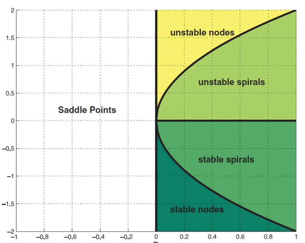
2 Classification trace determinant Kaper & Engler, 213

3 Topological Classification If neither eigenvalue has zero real part, then the system is called hyperbolic, in which case, there are only three classes: 1. saddles: One positive eigenvalue and one negative. The determinant is negative. 2. sources: Both eigenvalues have positive real part. The determinant is positive, and the trace is positive. 3. sinks: Both eigenvalues have negative real part. The determinant is positive, and the trace is negative. Every system in one of the three categories looks the same to a topologist (topological conjugacy).

4 Topological Classification saddle source trace sink determinant

5 Topological Classification Saddles : det < saddle source trace/ trace determinant 1 sink 1 determinant

6 Topological Classification Saddles : det < source saddle trace sink determinant

7 Topological Classification Sources det >, trace > saddle source trace trace determinant 1 sink 1 determinant

8 Topological Classification Sources det >, trace > source saddle trace sink determinant

9 Topological Classification Sinks det >, trace < saddle source trace trace determinant 1 sink 1 determinant

10 Topological Classification Sinks det >, trace < source saddle trace sink determinant

11 Topological Classification All sources look the same. Everything leaves.

12 Topological Classification All sinks look the same. Everything approaches the origin asymptotically.

13 Topological Classification One Variable x u u Let x u u u u u u 1 du u x u du u 1 Continuous, but not smooth at. u x du 1 du u u x 1 x u u du u

14 Topological Classification Two Variables Saddles dy x x 1 x u u 1 y v v du dv u v Continuous, but not smooth at (,). topologically conjugate

15 Topological Classification Sinks dy x x 1 x u u 1 y v v du dv u v Continuous, but not smooth at (,). topologically conjugate

16 Topological Classification What about spirals? dz ( 1 ) ix i ilog w z w we w Continuous, but not smooth at. dw w

17 Topological Classification Computation i dz i i 21 ( 1 iz ) ( ) i i 2 i 2 i 21 i i 2 i 2 z w w ww w w w dz z w ww w w w 2 2 i Multiply by w w i i i 1 i w 2 w w w w 2 w complex conjugate i i (1 iz ) (1 i) w w 1 ww i ww (1 i) ww ww ww 2ww i i 1 ww ww 2 ww (1 i) ww i i 2 2 ww 1 ww (1 i) ww ww ww 2ww ww iww (1 i) ww ww ww dw w add

18 Topological Classification What about spirals? dz ( 1 ) ix i ilog w z w we w Continuous, but not smooth at. dw w

19 Topological Classification All sinks are topologically conjugate, as are all sources and all saddles.

20 Topological Classification saddle source trace sink determinant

21 Rest points: Dynamical Systems Nonlinear Systems One Variable f ( x) f( x) If f( p), then x( t) p (constant) is a solution. Example x x 3 Rest points: 3 x x x 1 x 1 x 1,, and 1

22 Nonlinear Systems One Variable Rest points Example 2 x x 3 1 f(x) What about the stability of the rest points? x

23 Nonlinear Systems One Variable Rest points Example 2 x x 3 1 f(x) What about the stability of the rest points? x

24 Nonlinear Systems f ( x) Rest point p : f( p) Linear approximation: f ( x) f ( p) f ( p)( x p) f ( p)( x p) Introduce x p. Then f( x) f( p ) f( p) d f( x) f( p ) f( p) Basic Idea If is small, i.e., if x is close to p, d then solutions of f( p) d are close to solutions of f ( p). In particular, the rest point p is asymptotically stable for f ( x) d if the origin is asymptotically stable for f( p).

25 Nonlinear Systems f ( x) Rest point p : f( p) Criteria The rest point p is asymptotically stable for f( x) if f( p). It is unstable if f( p).

26 Nonlinear Systems Example f ( x) x x 3 2 stable Rest points: 1,, and 1 f( x) 13x f( 1) f(1) 2, f() 1 Rest points 1 and 1 are stable, rest point is unstable. 2 f(x) x unstable

27 Nonlinear Systems Two Variables 1 f1( x1, x2) 2 f2( x1, x2) f( x), x, f : f( x) If f( p), then x( t) p (constant) is a solution (rest point) f( p) f ( p, p ) f ( p, p ) x () t p 1 1 x () t p 1 1

28 Nonlinear Systems dy Example 3 x x y y Rest points: x x 3 y x x 3 x 1 x 1 x y y y ( 1,), (,), and (1,)

29 If y(), then y( t), for all t. invariant line : x axis Dynamical Systems Nonlinear Systems Example dy 3 x x y y y rest points x How do we analyze the full system?

30 Nonlinear Systems 3 x x y dy y Preview

31 Nonlinear Systems Jacobian Matrix 1 2 f ( x, x ) f ( x, x ) f( x), x, f : Df ( x) f1 f1 ( x1, x2) ( x1, x2) x1 x 2 f2 f ( x 2 1, x2) ( x1, x2) x1 x 2

32 Nonlinear Systems Example dy 3 x x y y Df ( x, y) 2 1 3x Df ( 1,) Df (,) Df (1,) 1 1 1

33 Nonlinear Systems f ( x) Rest point p : f( p) Linear approximation: f ( x) f ( p) Df ( p)( x p) Df ( p)( x p) Introduce x p. Then f( x) f( p ) Df( p) d f( x) f( p ) Df( p) Basic Idea If is small, i.e., if x is close to p, d then solutions of f( p) d are close to solutions of Df ( p). In particular, the rest point p is asymptotically stable for f ( x) d if the origin is asymptotically stable for Df ( p).

34 Nonlinear Systems f ( x) Rest point p : f( p) Criteria The rest point p is saddle for f( x) if det D f( p). It is a source if det D ( ) and trace D ( ). f p f p f p f p It is a source if det D ( ) and trace D ( ).

35 dy Dynamical Systems 3 x x y y Nonlinear Systems Example Rest points: ( 1,), (,), and (1,) Df ( 1,) Df (,) Df (1,) det D f ( 1,) 2 trace D f ( 1,) 3 sink 2 discriminant D f ( 1,) ( 3) det D f (,) 1 saddle stable node

36 If y(), then y( t), for all t. invariant line : x axis Dynamical Systems Nonlinear Systems Example dy 3 x x y y y rest points x stable node saddle