EAD 115. Numerical Solution of Engineering and Scientific Problems. David M. Rocke Department of Applied Science
|
|
|
- Georgia Higgins
- 5 years ago
- Views:
Transcription
1 EAD 115 Numerical Solution of Engineering and Scientific Problems David M. Rocke Department of Applied Science
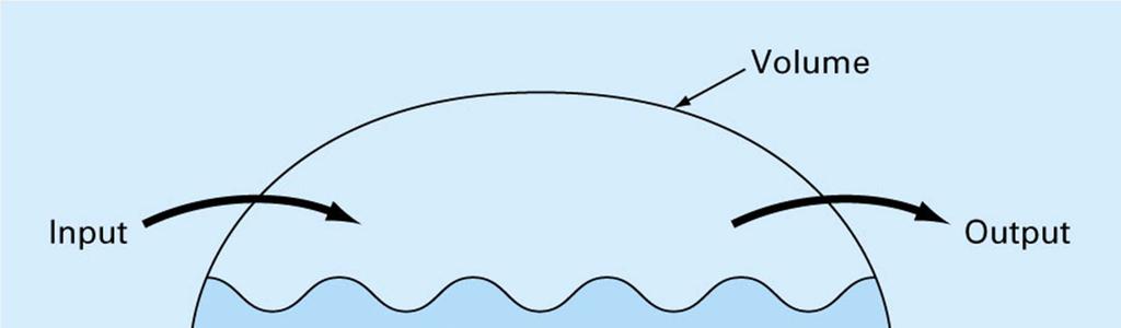
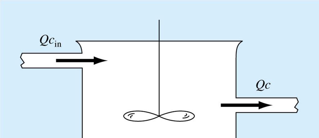
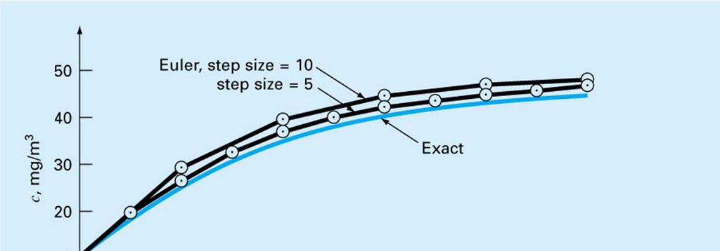
2 Transient Response of a Chemical Reactor Concentration of a substance in a chemical reactor can change during transient periods after startup or change in conditions Accumulation = inputs outputs V = volume of the reactor, assumed constant c = concentration of the substance, which can change.

3
4
5 Accumulation dc V dt in 0 Qc in Qc 1 ( Q/ V) t ( Q/ V) t in 0 cc e c e c Q 50mg/m 3 5m / min V=100m c 3 10mg/m t 0.05t c50 1e 10e
6
7 dc 1 c1 c3 dt
8 dc1 V1 Q01c01Q31c3 Q12c1Q15c1 dt dc1 0.12c1 0.02c3 1 dt dc2 0.15c10.15c2 dt dc c c3 4 dt dc4 0.1c c c5 dt dc5 0.3c10.01c2 0.04c5 dt c (0) c (0) c (0) c (0) c (0)


9 Solution using a fourth-order Runge-Kutta method. We can describe the response in terms of the time to 90% of the equilibrium concentration. This varies from about 12 for c 3 to over 70 for c 5


10 dc 1 c1 c3 dt
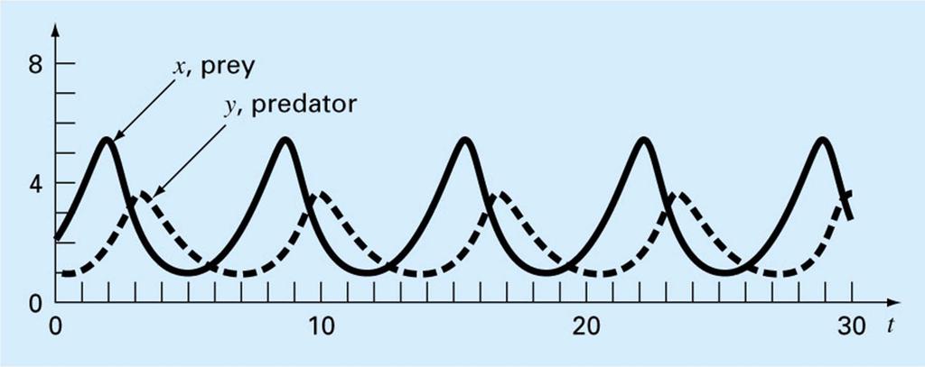
11 Predator-Prey Models Volterra-Lotka describe the reaction dynamics in an ecosystem In the simplest case, we let x represent the number of prey animals (rabbits) and y the number of predator animals (foxes). Rabbits naturally increase, and are assumed to have an adequate food supply, but are reduced by predation. Foxes increase only if there is adequate prey.
12 dx dt dy dt ax bxy cydxy Rabbits increase at a natural (birth death) rate a. Rabbits are reduced by a percentage by that depends on the number of foxes. Foxes reproduce at a rate dx dependent on the food supply. Foxes die at a rate c.
13
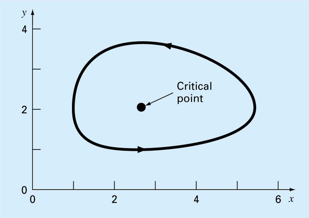
14 State-Space Representation The previous plot showed x and y against t. The state-space plot shows y against x This shows the stability, or lack of it, and the dynamics in a more concrete way
15
16 dx ax bxy 0 dt dy cydxy 0 dt x0 or aby y 0 or cdx (0,0) or (c/d, a/b)
17 Stochastic version dx dt dy dt ax bxy cydxy Critical point is not stable. Extinction can occur
18 Stochastic dynamics after 5 time periods
19 Stochastic dynamics after 10 time periods
20 Stochastic dynamics after 30 time periods
21 Simulating Transient Current in an Electric Circuit
22 di q L Ri E( t) 0 (Kirkoff's Law) dt C di L voltage drop across the inductor dt L inductance R resistance (of the resistor) = 0 q charge on the capacitor C capacitance (of the capacitor) Et ( ) time-varying voltage source = E0 sint dq i dt E0 E0 qt () sinpt sin t where p1/ LC L( p ) p L( p )
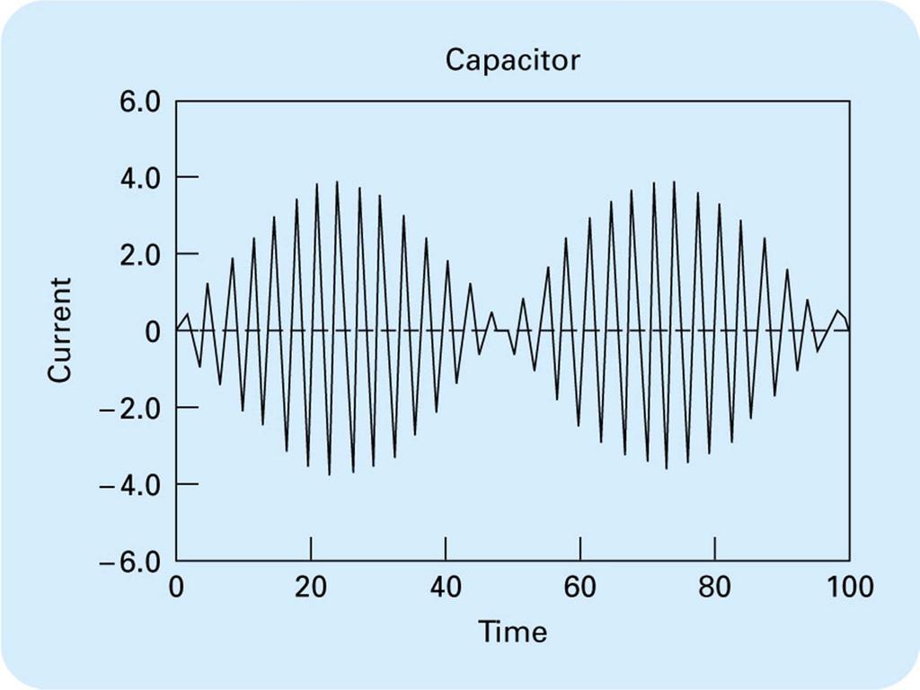
23
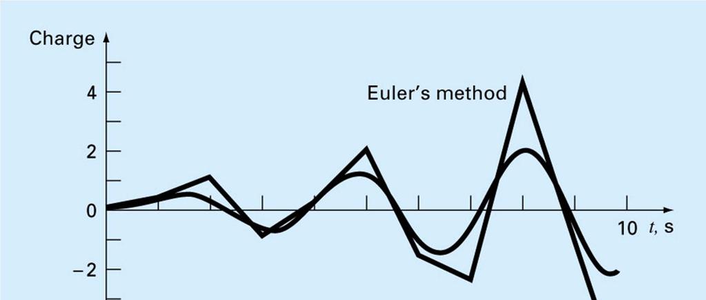
24 Assume L = 1H, E 0 = 1V, C = 0.25C, ω 2 = 3.5s 2, so that p = 2. q(t) = sin(2t) + 2 sin(1.8708t) Although an analytical solution exists, try integration with Euler and RK 4 methods Use h = 0.1s, evaluate accuracy at t = 10s. q(t) = C (exact) q(t) (Euler) q(t) (RK4)
25
26 The Swinging Pendulum The usual analysis of a swinging pendulum is an approximation which is valid for small arcs. We compare the exact solution of the approximate problem with an approximate solution of a more realistic model We do still model this as a point mass on a weightless, inextensible rod, so it is not completely realistic.
27
28 The force on the weight in the direction x tangent to the path is W F Wsin a g The angular acceleration in terms of the length l of the rod is 2 d a/ l 2 dt 2 Wl Wl d W sin 2 g g dt 2 d g sin 0 2 dt l
29 Exact solution to an approximation when is small sin 3! 5! 7! d 2 dt 2 g l () t cos 0 0 g t l The period of the pendulum is then T 2 l g
30 T 2 l g l 2ft 0 /4 (45) T s
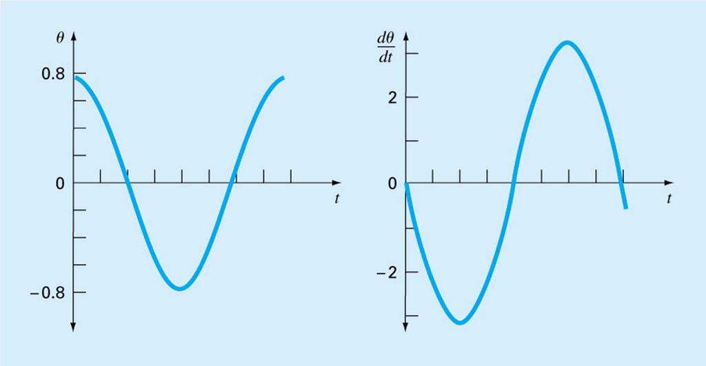
31
32 An approximate (numerical) solution to a more accurate physical model 2 d g sin 0 2 dt l d v dt dv g sin 16.1sin (for l 2ft) dt l Approximate with Euler method and standard order 4 Runge-Kutta method
33 k 1 Standard Fourth-Order Method f( x, y ) i k f( x h/2, y kh/2) 2 i i 1 k f( x h/2, y k h/2) 3 i i 2 k f( x h, y k h) 4 i i 3 i y y ( k 2k 2 k k ) h/6 i1 i
34 k f ( t, θ, v ) v k f ( t, θ, v ) 16.1sinθ 16.1sin π/ sin θ θ 0.005k θ 0.005(0) π/ * v v 0.005k ( ) k * f ( t, θ, v * * * * * * * * * * ) v k f ( t, θ, v ) 16.1sin θ θ θ 0.005k v v 0.005k
35 θ θ 0.005k * v v 0.005k * k f ( t, θ, v ) v * * * * k f ( t, θ, v ) 16.1sinθ * * * * θ θ 0.01k * v v 0.01k k * f ( t, θ * * * * * * * * , v ) v k f ( t, θ, v ) 16.1sinθ φ k 2k 2k 2k φ k 2k 2k 2k θ θ 0.01φ v v 0.01φ
36 Time Linear Euler h=0.05 RK 4 h=0.05 RK 4 h=
37 Analysis of Numerical Solutions The Euler method with h = 0.05 generates a impossible results at times t = 0.8, 1.0, and 1.6 The RK4 solutions with h = 0.05 and h = 0.01 are the same to 4 decimal places, suggesting the accuracy of the latter is at least that good. The RK4 h = 0.01 solution attains a max of at t = 1.63 compared to at the initial conditions Thus the difference between the linear approximation and the RK 4 solution can safely be interpreted.
38 Period Initial Displacement Linear Model Exact Nonlinear Model RK4 π/ π/ π/
39 An approximate solution to the exact problem is often better in a practical sense than the exact solution to an approximate problem. The art is in knowing how much to include in the model, and how accurate an approximate solution is required.
Math 128A Spring 2003 Week 12 Solutions
 Math 128A Spring 2003 Week 12 Solutions Burden & Faires 5.9: 1b, 2b, 3, 5, 6, 7 Burden & Faires 5.10: 4, 5, 8 Burden & Faires 5.11: 1c, 2, 5, 6, 8 Burden & Faires 5.9. Higher-Order Equations and Systems
Outline. Calculus for the Life Sciences. What is a Differential Equation? Introduction. Lecture Notes Introduction to Differential Equa
 Outline Calculus for the Life Sciences Lecture Notes to Differential Equations Joseph M. Mahaffy, jmahaffy@mail.sdsu.edu 1 Department of Mathematics and Statistics Dynamical Systems Group Computational
2.4 Harmonic Oscillator Models
 2.4 Harmonic Oscillator Models In this section we give three important examples from physics of harmonic oscillator models. Such models are ubiquitous in physics, but are also used in chemistry, biology,
2.4 Models of Oscillation
 2.4 Models of Oscillation In this section we give three examples of oscillating physical systems that can be modeled by the harmonic oscillator equation. Such models are ubiquitous in physics, but are
2D-Volterra-Lotka Modeling For 2 Species
 Majalat Al-Ulum Al-Insaniya wat - Tatbiqiya 2D-Volterra-Lotka Modeling For 2 Species Alhashmi Darah 1 University of Almergeb Department of Mathematics Faculty of Science Zliten Libya. Abstract The purpose
Homework #5 Solutions
 Homework #5 Solutions Math 123: Mathematical Modeling, Spring 2019 Instructor: Dr. Doreen De Leon 1. Exercise 7.2.5. Stefan-Boltzmann s Law of Radiation states that the temperature change dt/ of a body
Applications of Second-Order Differential Equations
 Applications of Second-Order Differential Equations ymy/013 Building Intuition Even though there are an infinite number of differential equations, they all share common characteristics that allow intuition
Elementary Differential Equations
 Elementary Differential Equations George Voutsadakis 1 1 Mathematics and Computer Science Lake Superior State University LSSU Math 310 George Voutsadakis (LSSU) Differential Equations January 2014 1 /
28. Pendulum phase portrait Draw the phase portrait for the pendulum (supported by an inextensible rod)
") 28. Pendulum phase portrait Draw the phase portrait for the pendulum (supported by an inextensible rod) θ + ω 2 sin θ = 0. Indicate the stable equilibrium points as well as the unstable equilibrium points.
28. Pendulum phase portrait Draw the phase portrait for the pendulum (supported by an inextensible rod) θ + ω 2 sin θ = 0. Indicate the stable equilibrium points as well as the unstable equilibrium points.
APPLICATIONS OF SECOND-ORDER DIFFERENTIAL EQUATIONS
 APPLICATIONS OF SECOND-ORDER DIFFERENTIAL EQUATIONS Second-order linear differential equations have a variety of applications in science and engineering. In this section we explore two of them: the vibration
Inductance, Inductors, RL Circuits & RC Circuits, LC, and RLC Circuits
 Inductance, Inductors, RL Circuits & RC Circuits, LC, and RLC Circuits Self-inductance A time-varying current in a circuit produces an induced emf opposing the emf that initially set up the timevarying
MEM 255 Introduction to Control Systems: Modeling & analyzing systems
 MEM 55 Introduction to Control Systems: Modeling & analyzing systems Harry G. Kwatny Department of Mechanical Engineering & Mechanics Drexel University Outline The Pendulum Micro-machined capacitive accelerometer
sections June 11, 2009
 sections 3.2-3.5 June 11, 2009 Population growth/decay When we model population growth, the simplest model is the exponential (or Malthusian) model. Basic ideas: P = P(t) = population size as a function
ECE2262 Electric Circuit
 ECE2262 Electric Circuit Chapter 7: FIRST AND SECOND-ORDER RL AND RC CIRCUITS Response to First-Order RL and RC Circuits Response to Second-Order RL and RC Circuits 1 2 7.1. Introduction 3 4 In dc steady
Math 266: Ordinary Differential Equations
 Math 266: Ordinary Differential Equations Long Jin Purdue University, Spring 2018 Basic information Lectures: MWF 8:30-9:20(111)/9:30-10:20(121), UNIV 103 Instructor: Long Jin (long249@purdue.edu) Office
1 Phasors and Alternating Currents
 Physics 4 Chapter : Alternating Current 0/5 Phasors and Alternating Currents alternating current: current that varies sinusoidally with time ac source: any device that supplies a sinusoidally varying potential
ENGI 3424 First Order ODEs Page 1-01
 ENGI 344 First Order ODEs Page 1-01 1. Ordinary Differential Equations Equations involving only one independent variable and one or more dependent variables, together with their derivatives with respect
Definition of differential equations and their classification. Methods of solution of first-order differential equations
 Introduction to differential equations: overview Definition of differential equations and their classification Solutions of differential equations Initial value problems Existence and uniqueness Mathematical
REACTANCE. By: Enzo Paterno Date: 03/2013
 REACTANCE REACTANCE By: Enzo Paterno Date: 03/2013 5/2007 Enzo Paterno 1 RESISTANCE - R i R (t R A resistor for all practical purposes is unaffected by the frequency of the applied sinusoidal voltage or
Systems of Differential Equations: General Introduction and Basics
 36 Systems of Differential Equations: General Introduction and Basics Thus far, we have been dealing with individual differential equations But there are many applications that lead to sets of differential
Chapter 10: Sinusoidal Steady-State Analysis
 Chapter 10: Sinusoidal Steady-State Analysis 1 Objectives : sinusoidal functions Impedance use phasors to determine the forced response of a circuit subjected to sinusoidal excitation Apply techniques
To find the step response of an RC circuit
 To find the step response of an RC circuit v( t) v( ) [ v( t) v( )] e tt The time constant = RC The final capacitor voltage v() The initial capacitor voltage v(t ) To find the step response of an RL circuit
Physics: spring-mass system, planet motion, pendulum. Biology: ecology problem, neural conduction, epidemics
 Applications of nonlinear ODE systems: Physics: spring-mass system, planet motion, pendulum Chemistry: mixing problems, chemical reactions Biology: ecology problem, neural conduction, epidemics Economy:
Handout 11: AC circuit. AC generator
 Handout : AC circuit AC generator Figure compares the voltage across the directcurrent (DC) generator and that across the alternatingcurrent (AC) generator For DC generator, the voltage is constant For
Wave Phenomena Physics 15c
 Wave Phenomena Physics 15c Lecture Harmonic Oscillators (H&L Sections 1.4 1.6, Chapter 3) Administravia! Problem Set #1! Due on Thursday next week! Lab schedule has been set! See Course Web " Laboratory
Electric Circuit Theory
 Electric Circuit Theory Nam Ki Min nkmin@korea.ac.kr 010-9419-2320 Chapter 8 Natural and Step Responses of RLC Circuits Nam Ki Min nkmin@korea.ac.kr 010-9419-2320 8.1 Introduction to the Natural Response
Lesson 9: Predator-Prey and ode45
 Lesson 9: Predator-Prey and ode45 9.1 Applied Problem. In this lesson we will allow for more than one population where they depend on each other. One population could be the predator such as a fox, and
(competition between 2 species) (Laplace s equation, potential theory,electricity) dx4 (chemical reaction rates) (aerodynamics, stress analysis)
 (Laplace s equation, potential theory,electricity) dx4 (chemical reaction rates) (aerodynamics, stress analysis)") SSE1793: Tutorial 1 1 UNIVERSITI TEKNOLOGI MALAYSIA SSE1793 DIFFERENTIAL EQUATIONS TUTORIAL 1 1. Classif each of the following equations as an ordinar differential equation (ODE) or a partial differential
SSE1793: Tutorial 1 1 UNIVERSITI TEKNOLOGI MALAYSIA SSE1793 DIFFERENTIAL EQUATIONS TUTORIAL 1 1. Classif each of the following equations as an ordinar differential equation (ODE) or a partial differential
Introduction to AC Circuits (Capacitors and Inductors)
") Introduction to AC Circuits (Capacitors and Inductors) Amin Electronics and Electrical Communications Engineering Department (EECE) Cairo University elc.n102.eng@gmail.com http://scholar.cu.edu.eg/refky/
Introduction to AC Circuits (Capacitors and Inductors) Amin Electronics and Electrical Communications Engineering Department (EECE) Cairo University elc.n102.eng@gmail.com http://scholar.cu.edu.eg/refky/
SCHOOL OF MATHEMATICS MATHEMATICS FOR PART I ENGINEERING. Self-paced Course
 SCHOOL OF MATHEMATICS MATHEMATICS FOR PART I ENGINEERING Self-paced Course MODULE 26 APPLICATIONS TO ELECTRICAL CIRCUITS Module Topics 1. Complex numbers and alternating currents 2. Complex impedance 3.
2.1 Exponential Growth
 2.1 Exponential Growth A mathematical model is a description of a real-world system using mathematical language and ideas. Differential equations are fundamental to modern science and engineering. Many
First-order transient
 EIE209 Basic Electronics First-order transient Contents Inductor and capacitor Simple RC and RL circuits Transient solutions Constitutive relation An electrical element is defined by its relationship between
Graded Project #1. Part 1. Explicit Runge Kutta methods. Goals Differential Equations FMN130 Gustaf Söderlind and Carmen Arévalo
 2008-11-07 Graded Project #1 Differential Equations FMN130 Gustaf Söderlind and Carmen Arévalo This homework is due to be handed in on Wednesday 12 November 2008 before 13:00 in the post box of the numerical
Motivation and Goals. Modelling with ODEs. Continuous Processes. Ordinary Differential Equations. dy = dt
 Motivation and Goals Modelling with ODEs 24.10.01 Motivation: Ordinary Differential Equations (ODEs) are very important in all branches of Science and Engineering ODEs form the basis for the simulation
SYSTEMS OF ODES. mg sin ( (x)) dx 2 =
) dx 2 =") SYSTEMS OF ODES Consider the pendulum shown below. Assume the rod is of neglible mass, that the pendulum is of mass m, and that the rod is of length `. Assume the pendulum moves in the plane shown, and
SYSTEMS OF ODES Consider the pendulum shown below. Assume the rod is of neglible mass, that the pendulum is of mass m, and that the rod is of length `. Assume the pendulum moves in the plane shown, and
Chapter 6. Second order differential equations
 Chapter 6. Second order differential equations A second order differential equation is of the form y = f(t, y, y ) where y = y(t). We shall often think of t as parametrizing time, y position. In this case
Inductance, RL and RLC Circuits
 Inductance, RL and RLC Circuits Inductance Temporarily storage of energy by the magnetic field When the switch is closed, the current does not immediately reach its maximum value. Faraday s law of electromagnetic
2 Growth, Decay, and Oscillation
 2 Growth, Decay, and Oscillation b The city of Suzhou in Jiangsu Province, China. Suzhou is the fastest growing city in the world, with an annual population growth of 6.5% between the years 2000 and 2014.1
Module 25: Outline Resonance & Resonance Driven & LRC Circuits Circuits 2
 Module 25: Driven RLC Circuits 1 Module 25: Outline Resonance & Driven LRC Circuits 2 Driven Oscillations: Resonance 3 Mass on a Spring: Simple Harmonic Motion A Second Look 4 Mass on a Spring (1) (2)
Wave Phenomena Physics 15c
 Wave Phenomena Physics 15c Lecture Harmonic Oscillators (H&L Sections 1.4 1.6, Chapter 3) Administravia! Problem Set #1! Due on Thursday next week! Lab schedule has been set! See Course Web " Laboratory
Solution to Homework 2
 Solution to Homework. Substitution and Nonexact Differential Equation Made Exact) [0] Solve dy dx = ey + 3e x+y, y0) = 0. Let u := e x, v = e y, and hence dy = v + 3uv) dx, du = u)dx, dv = v)dy = u)dv
Computers, Lies and the Fishing Season
 1/47 Computers, Lies and the Fishing Season Liz Arnold May 21, 23 Introduction Computers, lies and the fishing season takes a look at computer software programs. As mathematicians, we depend on computers
Module 24: Outline. Expt. 8: Part 2:Undriven RLC Circuits
 Module 24: Undriven RLC Circuits 1 Module 24: Outline Undriven RLC Circuits Expt. 8: Part 2:Undriven RLC Circuits 2 Circuits that Oscillate (LRC) 3 Mass on a Spring: Simple Harmonic Motion (Demonstration)
EE292: Fundamentals of ECE
 EE292: Fundamentals of ECE Fall 2012 TTh 10:00-11:15 SEB 1242 Lecture 14 121011 http://www.ee.unlv.edu/~b1morris/ee292/ 2 Outline Review Steady-State Analysis RC Circuits RL Circuits 3 DC Steady-State
4.2 Homogeneous Linear Equations
 4.2 Homogeneous Linear Equations Homogeneous Linear Equations with Constant Coefficients Consider the first-order linear differential equation with constant coefficients a 0 and b. If f(t) = 0 then this
Inductance, RL Circuits, LC Circuits, RLC Circuits
 Inductance, R Circuits, C Circuits, RC Circuits Inductance What happens when we close the switch? The current flows What does the current look like as a function of time? Does it look like this? I t Inductance
EE292: Fundamentals of ECE
 EE292: Fundamentals of ECE Fall 2012 TTh 10:00-11:15 SEB 1242 Lecture 20 121101 http://www.ee.unlv.edu/~b1morris/ee292/ 2 Outline Chapters 1-3 Circuit Analysis Techniques Chapter 10 Diodes Ideal Model
Physics 208, Spring 2016 Exam #3
 Physics 208, Spring 206 Exam #3 A Name (Last, First): ID #: Section #: You have 75 minutes to complete the exam. Formulae are provided on an attached sheet. You may NOT use any other formula sheet. You
11. AC Circuit Power Analysis
 . AC Circuit Power Analysis Often an integral part of circuit analysis is the determination of either power delivered or power absorbed (or both). In this chapter First, we begin by considering instantaneous
Chapter 33. Alternating Current Circuits
 Chapter 33 Alternating Current Circuits 1 Capacitor Resistor + Q = C V = I R R I + + Inductance d I Vab = L dt AC power source The AC power source provides an alternative voltage, Notation - Lower case
RLC Series Circuit. We can define effective resistances for capacitors and inductors: 1 = Capacitive reactance:
 RLC Series Circuit In this exercise you will investigate the effects of changing inductance, capacitance, resistance, and frequency on an RLC series AC circuit. We can define effective resistances for
MATH 250 Homework 4: Due May 4, 2017
 Due May 4, 17 Answer the following questions to the best of your ability. Solutions should be typed. Any plots or graphs should be included with the question (please include the questions in your solutions).
Chapter 4 Transients. Chapter 4 Transients
 Chapter 4 Transients Chapter 4 Transients 1. Solve first-order RC or RL circuits. 2. Understand the concepts of transient response and steady-state response. 1 3. Relate the transient response of first-order
Chapter 2 PARAMETRIC OSCILLATOR
 CHAPTER- Chapter PARAMETRIC OSCILLATOR.1 Introduction A simple pendulum consists of a mass m suspended from a string of length L which is fixed at a pivot P. When simple pendulum is displaced to an initial
Ordinary Differential Equations (ODE)
") Ordinary Differential Equations (ODE) Why study Differential Equations? Many physical phenomena are best formulated mathematically in terms of their rate of change. Motion of a swinging pendulum Bungee-jumper
Ordinary Differential Equations (ODE) Why study Differential Equations? Many physical phenomena are best formulated mathematically in terms of their rate of change. Motion of a swinging pendulum Bungee-jumper
Chapter 4. Systems of ODEs. Phase Plane. Qualitative Methods
 Chapter 4 Systems of ODEs. Phase Plane. Qualitative Methods Contents 4.0 Basics of Matrices and Vectors 4.1 Systems of ODEs as Models 4.2 Basic Theory of Systems of ODEs 4.3 Constant-Coefficient Systems.
Periodic motion Oscillations. Equilibrium position
 Periodic motion Oscillations Equilibrium position Any kinds of motion repeat themselves over and over: the vibration of a quartz crystal in a watch, the swinging pendulum of a grandfather clock, the sound
Lecture 35: FRI 17 APR Electrical Oscillations, LC Circuits, Alternating Current I
 Physics 3 Jonathan Dowling Lecture 35: FRI 7 APR Electrical Oscillations, LC Circuits, Alternating Current I Nikolai Tesla What are we going to learn? A road map Electric charge è Electric force on other
1.Introduction: 2. The Model. Key words: Prey, Predator, Seasonality, Stability, Bifurcations, Chaos.
 Dynamical behavior of a prey predator model with seasonally varying parameters Sunita Gakkhar, BrhamPal Singh, R K Naji Department of Mathematics I I T Roorkee,47667 INDIA Abstract : A dynamic model based
dx n a 1(x) dy
 dy") HIGHER ORDER DIFFERENTIAL EQUATIONS Theory of linear equations Initial-value and boundary-value problem nth-order initial value problem is Solve: a n (x) dn y dx n + a n 1(x) dn 1 y dx n 1 +... + a 1(x)
HIGHER ORDER DIFFERENTIAL EQUATIONS Theory of linear equations Initial-value and boundary-value problem nth-order initial value problem is Solve: a n (x) dn y dx n + a n 1(x) dn 1 y dx n 1 +... + a 1(x)
ECE2262 Electric Circuits. Chapter 6: Capacitance and Inductance
 ECE2262 Electric Circuits Chapter 6: Capacitance and Inductance Capacitors Inductors Capacitor and Inductor Combinations Op-Amp Integrator and Op-Amp Differentiator 1 CAPACITANCE AND INDUCTANCE Introduces
AC Circuits Homework Set
 Problem 1. In an oscillating LC circuit in which C=4.0 μf, the maximum potential difference across the capacitor during the oscillations is 1.50 V and the maximum current through the inductor is 50.0 ma.
7.3 State Space Averaging!
 7.3 State Space Averaging! A formal method for deriving the small-signal ac equations of a switching converter! Equivalent to the modeling method of the previous sections! Uses the state-space matrix description
Oscillations. Tacoma Narrow Bridge: Example of Torsional Oscillation
 Oscillations Mechanical Mass-spring system nd order differential eq. Energy tossing between mass (kinetic energy) and spring (potential energy) Effect of friction, critical damping (shock absorber) Simple
Lecture 6: Impedance (frequency dependent. resistance in the s- world), Admittance (frequency. dependent conductance in the s- world), and
, Admittance (frequency. dependent conductance in the s- world), and") Lecture 6: Impedance (frequency dependent resistance in the s- world), Admittance (frequency dependent conductance in the s- world), and Consequences Thereof. Professor Ray, what s an impedance? Answers:
Lecture 6: Impedance (frequency dependent resistance in the s- world), Admittance (frequency dependent conductance in the s- world), and Consequences Thereof. Professor Ray, what s an impedance? Answers:
Chapter 31 Electromagnetic Oscillations and Alternating Current LC Oscillations, Qualitatively
 Chapter 3 Electromagnetic Oscillations and Alternating Current LC Oscillations, Qualitatively In the LC circuit the charge, current, and potential difference vary sinusoidally (with period T and angular
P441 Analytical Mechanics - I. RLC Circuits. c Alex R. Dzierba. In this note we discuss electrical oscillating circuits: undamped, damped and driven.
 Lecture 10 Monday - September 19, 005 Written or last updated: September 19, 005 P441 Analytical Mechanics - I RLC Circuits c Alex R. Dzierba Introduction In this note we discuss electrical oscillating
Coordinate Curves for Trajectories
 43 The material on linearizations and Jacobian matrices developed in the last chapter certainly expanded our ability to deal with nonlinear systems of differential equations Unfortunately, those tools
Ordinary Differential Equations
 Ordinary Differential Equations Michael H. F. Wilkinson Institute for Mathematics and Computing Science University of Groningen The Netherlands December 2005 Overview What are Ordinary Differential Equations
Second order differential equations 4
 A course in differential equations Chapter 3. Second order differential equations A second order differential equation is of the form y 00 = F (t; y; y 0 ) where y = y(t). We shall often think of t as
Electric Circuit Theory
 Electric Circuit Theory Nam Ki Min nkmin@korea.ac.kr 010-9419-2320 Chapter 11 Sinusoidal Steady-State Analysis Nam Ki Min nkmin@korea.ac.kr 010-9419-2320 Contents and Objectives 3 Chapter Contents 11.1
Differential Equations and Linear Algebra Supplementary Notes. Simon J.A. Malham. Department of Mathematics, Heriot-Watt University
 Differential Equations and Linear Algebra Supplementary Notes Simon J.A. Malham Department of Mathematics, Heriot-Watt University Contents Chapter 1. Linear algebraic equations 5 1.1. Gaussian elimination
Numerical Methods for ODEs. Lectures for PSU Summer Programs Xiantao Li
 Numerical Methods for ODEs Lectures for PSU Summer Programs Xiantao Li Outline Introduction Some Challenges Numerical methods for ODEs Stiff ODEs Accuracy Constrained dynamics Stability Coarse-graining
Chap. 20: Initial-Value Problems
 Chap. 20: Initial-Value Problems Ordinary Differential Equations Goal: to solve differential equations of the form: dy dt f t, y The methods in this chapter are all one-step methods and have the general
PES 1120 Spring 2014, Spendier Lecture 35/Page 1
 PES 0 Spring 04, Spendier Lecture 35/Page Today: chapter 3 - LC circuits We have explored the basic physics of electric and magnetic fields and how energy can be stored in capacitors and inductors. We
Announcements: Today: more AC circuits
 Announcements: Today: more AC circuits I 0 I rms Current through a light bulb I 0 I rms I t = I 0 cos ωt I 0 Current through a LED I t = I 0 cos ωt Θ(cos ωt ) Theta function (is zero for a negative argument)
XXIX Applications of Differential Equations
 MATHEMATICS 01-BNK-05 Advanced Calculus Martin Huard Winter 015 1. Suppose that the rate at which a population of size yt at time t changes is proportional to the amount present. This gives rise to the
Inductive & Capacitive Circuits. Subhasish Chandra Assistant Professor Department of Physics Institute of Forensic Science, Nagpur
 Inductive & Capacitive Circuits Subhasish Chandra Assistant Professor Department of Physics Institute of Forensic Science, Nagpur LR Circuit LR Circuit (Charging) Let us consider a circuit having an inductance
Math 128A Spring 2003 Week 11 Solutions Burden & Faires 5.6: 1b, 3b, 7, 9, 12 Burden & Faires 5.7: 1b, 3b, 5 Burden & Faires 5.
 Math 128A Spring 2003 Week 11 Solutions Burden & Faires 5.6: 1b, 3b, 7, 9, 12 Burden & Faires 5.7: 1b, 3b, 5 Burden & Faires 5.8: 1b, 3b, 4 Burden & Faires 5.6. Multistep Methods 1. Use all the Adams-Bashforth
MAT01B1: Separable Differential Equations
 MAT01B1: Separable Differential Equations Dr Craig 3 October 2018 My details: acraig@uj.ac.za Consulting hours: Tomorrow 14h40 15h25 Friday 11h20 12h55 Office C-Ring 508 https://andrewcraigmaths.wordpress.com/
CDS 101: Lecture 2.1 System Modeling
 CDS 101: Lecture 2.1 System Modeling Richard M. Murray 4 October 2004 Goals: Define what a model is and its use in answering questions about a system Introduce the concepts of state, dynamics, inputs and
 Alternating Currents. The power is transmitted from a power house on high voltage ac because (a) Electric current travels faster at higher volts (b) It is more economical due to less power wastage (c)
Module 4. Single-phase AC Circuits
 Module 4 Single-phase AC Circuits Lesson 14 Solution of Current in R-L-C Series Circuits In the last lesson, two points were described: 1. How to represent a sinusoidal (ac) quantity, i.e. voltage/current
Alternating Current Circuits
 Alternating Current Circuits AC Circuit An AC circuit consists of a combination of circuit elements and an AC generator or source. The output of an AC generator is sinusoidal and varies with time according
ELECTRONICS E # 1 FUNDAMENTALS 2/2/2011
 FE Review 1 ELECTRONICS E # 1 FUNDAMENTALS Electric Charge 2 In an electric circuit it there is a conservation of charge. The net electric charge is constant. There are positive and negative charges. Like
ECEN 420 LINEAR CONTROL SYSTEMS. Lecture 6 Mathematical Representation of Physical Systems II 1/67
 1/67 ECEN 420 LINEAR CONTROL SYSTEMS Lecture 6 Mathematical Representation of Physical Systems II State Variable Models for Dynamic Systems u 1 u 2 u ṙ. Internal Variables x 1, x 2 x n y 1 y 2. y m Figure
Modeling and Simulation Revision IV D R. T A R E K A. T U T U N J I P H I L A D E L P H I A U N I V E R S I T Y, J O R D A N
 Modeling and Simulation Revision IV D R. T A R E K A. T U T U N J I P H I L A D E L P H I A U N I V E R S I T Y, J O R D A N 2 0 1 7 Modeling Modeling is the process of representing the behavior of a real
Chapter 10: Sinusoids and Phasors
 Chapter 10: Sinusoids and Phasors 1. Motivation 2. Sinusoid Features 3. Phasors 4. Phasor Relationships for Circuit Elements 5. Impedance and Admittance 6. Kirchhoff s Laws in the Frequency Domain 7. Impedance
EE292: Fundamentals of ECE
 EE292: Fundamentals of ECE Fall 2012 TTh 10:00-11:15 SEB 1242 Lecture 18 121025 http://www.ee.unlv.edu/~b1morris/ee292/ 2 Outline Review RMS Values Complex Numbers Phasors Complex Impedance Circuit Analysis
Lecture 20/Lab 21: Systems of Nonlinear ODEs
 Lecture 20/Lab 21: Systems of Nonlinear ODEs MAR514 Geoffrey Cowles Department of Fisheries Oceanography School for Marine Science and Technology University of Massachusetts-Dartmouth Coupled ODEs: Species
Dynamic Modeling. For the mechanical translational system shown in Figure 1, determine a set of first order
 QUESTION 1 For the mechanical translational system shown in, determine a set of first order differential equations describing the system dynamics. Identify the state variables and inputs. y(t) x(t) k m
Getting Started With The Predator - Prey Model: Nullclines
 Getting Started With The Predator - Prey Model: Nullclines James K. Peterson Department of Biological Sciences and Department of Mathematical Sciences Clemson University October 28, 2013 Outline The Predator
HOMEWORK 4: MATH 265: SOLUTIONS. y p = cos(ω 0t) 9 ω 2 0
 9 ω 2 0") HOMEWORK 4: MATH 265: SOLUTIONS. Find the solution to the initial value problems y + 9y = cos(ωt) with y(0) = 0, y (0) = 0 (account for all ω > 0). Draw a plot of the solution when ω = and when ω = 3.
HOMEWORK 4: MATH 265: SOLUTIONS. Find the solution to the initial value problems y + 9y = cos(ωt) with y(0) = 0, y (0) = 0 (account for all ω > 0). Draw a plot of the solution when ω = and when ω = 3.
Modelling biological oscillations
 Modelling biological oscillations Shan He School for Computational Science University of Birmingham Module 06-23836: Computational Modelling with MATLAB Outline Outline of Topics Van der Pol equation Van
Noise - irrelevant data; variability in a quantity that has no meaning or significance. In most cases this is modeled as a random variable.
 1.1 Signals and Systems Signals convey information. Systems respond to (or process) information. Engineers desire mathematical models for signals and systems in order to solve design problems efficiently
Lecture - 11 Bendixson and Poincare Bendixson Criteria Van der Pol Oscillator
 Nonlinear Dynamical Systems Prof. Madhu. N. Belur and Prof. Harish. K. Pillai Department of Electrical Engineering Indian Institute of Technology, Bombay Lecture - 11 Bendixson and Poincare Bendixson Criteria
NOTICE TO CUSTOMER: The sale of this product is intended for use of the original purchaser only and for use only on a single computer system.
 NOTICE TO CUSTOMER: The sale of this product is intended for use of the original purchaser only and for use only on a single computer system. Duplicating, selling, or otherwise distributing this product
Physics for Scientists & Engineers 2
 Electromagnetic Oscillations Physics for Scientists & Engineers Spring Semester 005 Lecture 8! We have been working with circuits that have a constant current a current that increases to a constant current
= D. 5. The displacement s (in cm) of a linkage joint of a robot is given by s = (4t-t 2 ) 213, where t is. Find the derivative.
 of a linkage joint of a robot is given by s = (4t-t 2 ) 213, where t is. Find the derivative.") 1. Find the derivative. y=(5x+11) 3 = D 2. Find the derivative. y= (4x 3 +7) 312 = D 3. Find - for y = x(5x 2 + 3 ) 112. = D 4. Differentiate the given function. ( x - 1 3 y= --) x-7 = D 5. The displacement
1. Find the derivative. y=(5x+11) 3 = D 2. Find the derivative. y= (4x 3 +7) 312 = D 3. Find - for y = x(5x 2 + 3 ) 112. = D 4. Differentiate the given function. ( x - 1 3 y= --) x-7 = D 5. The displacement
second order Runge-Kutta time scheme is a good compromise for solving ODEs unstable for oscillators
 ODE Examples We have seen so far that the second order Runge-Kutta time scheme is a good compromise for solving ODEs with a good precision, without making the calculations too heavy! It is unstable for