Energy in General Relativity

Transcription

1 Energy in General Relativity Sergio Dain FaMAF-Universidad Nacional de Córdoba, CONICET, Argentina. March, / 137

2 Energy Energy is a central concept in Physics: it has many forms, it is always conserved. The energy concept provides a deep link between Physics and Mathematics. Mathematical applications of the energy concept: Uniqueness of solutions. Existence of solutions. Weak solutions: natural Sobolev spaces. Calculus of variations Energy estimates for evolution equations: stability of solutions. Energy in General Relativity: the Yamabe problem. 2 / 137

3 Physics vs Mathematics Physics: Using heuristic arguments, discover the mathematical formula for the energy of a given theory. And then guess some of its mathematically properties: positivity, conservation. Try to find physical interpretation and applications of mathematical interesting energy definitions. Mathematics: Prove the properties or find counter examples. Discover new connections between the energy and other mathematical concepts. Find new appliactions of the energy concept to solve other problems. Find new kind of energies, which are mathematically relevant. 3 / 137

4 Energy in General Relativity The physical concept of energy in General Relativity is subtle. It was not easy to discover the definition of total energy. Given the definition, to prove the positivity was remarkably difficult. From the geometrical energy definition, without the physical picture, it would be very hard even to conjecture that this quantity should be positive. 4 / 137

5 5 / 137

6 Plan of the lectures Part I: Energy in Electrodynamics. Part II: Energy in General Relativity. Definition, examples, meaning of the positive energy theorems, proofs in simple cases. Part III: Witten proof of the positive energy theorem. Part IV: Schoen-Yau proof of the positive energy theorem. 6 / 137

7 Bibliography Part I: Texts books in Electrodynamics: J. D. Jackson, Classical Electrodynamics, A. Zangwill, Modern Electrodynamics, O. Reula lectures notes: Electromagnetismo/electrodynamics.pdf Section 2 in L. B. Szabados Quasi-Local Energy-Momentum and Angular Momentum in General Relativity, Living Rev. Relativity 12, (2009). Part II: Based on my review article Positive energy theorems in General Relativity, Chapter 18 of The Springer Handbook of Spacetime, See also P. Chruściel Lectures Notes: teaching/energy/energy.pdf 7 / 137

8 Part III: Based on my review article Positive energy theorems in General Relativity, Chapter 18 of The Springer Handbook of Spacetime, Introduction to Spinors: R. Geroch Spinors, Chapter 15 of the same book. R. Wald General Relativity, Chapter 13. Penrose and Rindler Vol 1 Spinors and Space-Time. 8 / 137

9 Part IV: Mostly based on the original article: On the proof of the positive mass conjecture in general relativity, R. Schoen, S. T. Yau, Comm. Math. Phys., 65 (1), 45-76, M. Khuri lectures notes: Khuri-PMT.pdf For more about minimal surface: T. Colding, W. P. Minicozzi II, A course in minimal surfaces, / 137

10 PART I 10 / 137

11 Mechanics F : force on a particle. F = ma: Newton s Law. Work: 2 W 12 = 2 1 F ds 1 Work and kinetic energy: 2 1 F ds = 2 1 m dv dt v dt = m 2 = m 2 (v 2 (2) v 2 (1)). We define the kinetic energy of the particle by T = 1 2 mv 2, 2 1 d dt v 2 dt and hence previous equation is given by W 12 = T (2) T (1). The work done by the external force is equal to the change in the kinetic energy. 11 / 137

12 Assume that the force F is the gradient of a potential then F = Φ, W 12 = Φ(2) Φ(1). We define Φ to be the potential energy of the particule. The total energy of the particle is given by It is conserved: E = Φ + T. E(2) = E(1), d dt E = / 137

13 Electrostatic Electrostatic equations (Gaussian units): E = 0, E = 4πρ, where E is the electric field and ρ is the charge density. Potential: E = Φ, Φ = 4πρ. Electric force (definition of the electric field): Work: W 12 = 2 1 F = qe. F ds = q(φ(2) Φ(1)) If we take the point 2 at infinity and we chose the constant in the potential such that Φ( ) = 0, then the work needed to bring a charge q from infinity to the point x under the field E is given by W = qφ(x). 13 / 137

14 Binding Energy The work needed to place a density ρ on a external potential (i.e. not produced by ρ) is given by W = ρφ. We want to compute the work needed to assemble the charge density ρ. Let ρ and Φ be the final charge density and potential (produced by this density). Let λ [0, 1] a real number, and consider the density λρ and corresponding potential λφ. The work needed to bring a δρ from infinity under the field λφ is given by δw = δρ(λφ) = (δλ)ρ(λφ). Then, we deduce dw dλ = λρφ Integrating we obtain the total work required to build the system 1 dw 1 E = dλ dλ = ρφ λdλ = 1 ρφ / 137

15 Positivity of the binding energy Consider ρ of compact support in the region U E = 1 ρφ = 1 Φ Φ 2 U 8π U = 1 ( (Φ Φ) Φ 2 8π U = 1 Φ Φ 8π U n + 1 Φ 2 8π U = 1 Φ 2 8π R 3 = 1 E 2. 8π R 3 15 / 137

16 Application: uniqueness of solution in electrostatics Consider the Dirichlet boundary problem Φ = 4πρ in U, Φ = g in U. Assume we have two different solutions Φ 1 and Φ 2 with the same source and boundary data. Then the difference Φ = Φ 2 Φ 1 is solution of the homogeneous problem Φ = 0 in U, Φ = 0 in U. Then, That is 0 = U Φ Φ = U E(U) = Φ Φ n Φ 2. U U Φ Φ n. By the boundary condition at U we obtain E(U) = 0. Hence, Φ is constant in U and by the boundary condition we deduce is zero. 16 / 137

17 Electrodynamics Maxwell equations (Gaussian units) E + 1 B c t = 0, E = 4πρ, B 1 E c t = 4π J, B = 0. c Energy density of the electromagnetic field: Energy conservation: Poynting vector: e = 1 ( E 2 + B 2) 8π e t + S = J E, S = c 4π E B. 17 / 137

18 Lorentz force acting on a particle of charge q and velocity v: F = q(e + v c B) Work done by the force: dw dt = F v = J E. Energy conservation (non-covariant formulation): d (W + E) = S n dt U 18 / 137

19 Energy: covariant formulation Maxwell equations (Geometric units c = 1): µ F µν = 4πJ ν, [µ F νλ] = 0. Energy momentum tensor of the electromagnetic field T µν = 1 (F µλ F λ ν 14 ) 4π g µνf λγ F λγ, We assume J µ = 0. Properties of T µν : T µν = T νµ, T µ µ = 0, µ T µν = 0. T 00 = 1 8π ( E 2 + B 2 ) = e, T 0i = 1 4π (E B) i = S i 19 / 137

20 Let k µ be a Killing vector, i.e. (ν k µ) = 0. Then, the vector K µ defined by K µ = T µν k ν, is divergence free µ K µ = / 137

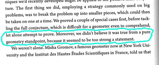
21 Stokes Theorem on Lorentzian Manifolds For a vector field K µ we have the identity µ K µ = K µ n µ. Ω Both integrals are taken with respect to the induced volume form. The vector n µ is the unit normal to Ω and its direction depends on the convention of the signature of the metric. For Lorentzian metrics with signature (, +, +, +) the vector n µ is the inward directed unit normal to Ω in case is spacelike and the outward directed unit normal in case Ω is timelike. If Ω is null then we take a past (future) directed null normal to Ω if it is future (past) boundary. Ω (picture from S. Aretakis) 21 / 137

22 Energy conditions Weak energy condition: T µν ξ µ ξ ν 0, for all timelike vectors ξ µ. Physical interpretation: T µν ξ µ ξ ν is the energy density measured by the observed ξ µ and it should be positive. Dominant energy condition: For all future directed timelike vector ξ µ the vector T µ νξ ν should be future directed timelike or null vector. Physical interpretation: T µ νξ ν is the energy momentum current density. The dominant energy condition implies that the speed of the energy flow is less or equal the speed of light. Equivalent formulation: T µν ξ µ k ν 0, for all future directed timelike or null vectors k µ and ξ µ. 22 / 137

23 Domains Let U be a 3-dimensional spacelike domain with (timelike) normal n µ we define the energy by E(U) = K µ n µ. Let C be a null or timelike 3-dimensional surface with (spacelike or null) normal n µ, we define the flux by F(C) = K µ n µ. U C 23 / 137

24 Timelike cylinder U 1 and U 2 spacelike surfaces t = constant (green surfaces). C timelike cylinder (blue surface). E(U 2 ) E(U 1 ) = F(C) The flux F(C) can have any sign: incoming or outgoing radiation. 24 / 137

25 Future domain of dependence U 1 and U 2 spacelike surfaces t = constant (green surfaces). C timelike cylinder (blue surface). E(U 2 ) E(U 1 ) = F(C) 0 The flux F(C) 0 is always negative: radiation can escape but can not enter the domain. 25 / 137

26 Past domain of dependence U 1 and U 2 spacelike surfaces t = constant (green surfaces). C timelike cylinder (blue surface). E(U 2 ) E(U 1 ) = F(C) 0 The flux F(C) 0 is always positive: radiation can enter but it can not escape. 26 / 137

27 Conservation of energy Assume that the initial data for the electromagnetic field has compact support. Define the total energy by E = 1 E 2 + B 2 8π R 3 then, we have d dt E = / 137

28 Linear momentum Given a plane t = constant we asociate a cartesian coordinates system to it (t, x, y, z). In this coordinate system we compute the following quantity P µ = T µν t ν, R 3 where t ν is the timelike normal to the plane. This quantity is a vector in the following sense: if we have another plane (t, x, y, z ) and compute P µ = T µνt ν, R 3 then P µ and P µ are related by a Lorentz transformation. 28 / 137

29 To prove this non-trivial statement we compute, for a constant but otherwise arbitrary vector k u P µ k µ = T µν k µ t ν R 3 Using the Gauss theorem we prove that We define the invariant P µ k µ = P µk µ. M = P µ P µ. 29 / 137

30 Aplication: uniqueness of the Cauchy problem in electrodynamics Given initial data E and B en t = 0 the solution of Maxwell equations is unique. Proof: assume there are two solutions, then the difference has zero initial data. Compute the energy, the energy is zero initially and, by conservation, is zero for all time. Then the difference is zero. 30 / 137

31 Aplication: stability for the wave equation Wave equation: Φ = 0. Energy for the wave equation E = Φ 2 + Φ 2 R 3 The energy is conserved d dt E = 0. If we take a time derivative to the wave equation we obtain Φ = 0. Then, the following energy is also conserved E 1 = Φ 2 + Φ 2 R 3 31 / 137

32 The solutions of the wave equation satisfies the following pointwise estimate Φ C(E + E 1 ), where C is a numerical constant that not depends on Φ. 32 / 137

33 PART II 33 / 137

34 Energy in General Relativity: introduction I will present an introduction and also an overview of some of the most relevant results concerning positivity energy theorems in General Relativity. These theorems provide the answer to a long standing problem that has been proved remarkably difficult to solve. They constitute one of the major results in classical General Relativity and they uncover a deep self-consistence of the theory. In this introduction I would like to present the theorems in a complete form but with the least possible amount of technical details, in such a way that you can have a rough idea of the basic ingredients. In the following lectures I will discuss the examples that illustrate the hypothesis of the theorems. 34 / 137

35 Isolated systems in General Relativity An isolated system is an idealization in physics that assumes that the sources are confined to a finite region and the fields are weak far away from the sources. This kind of systems are expected to have finite total energy. In General Relativity there are several ways of defining isolated systems. For our purpose the most appropriate definition is through initial conditions for Einstein equations. The reasons for that are twofold: The notion of total energy has been discovered and formulated using a Hamiltonian formulation of the theory which involves the study of initial conditions. The proofs of the positive mass theorem are mainly given in terms of initial conditions. 35 / 137

36 Initial data set Initial conditions for Einstein equations are characterized by initial data set given by (S, h ij, K ij, µ, j i ) where S is a connected 3-dimensional manifold, h ij a (positive definite) Riemannian metric, K ij a symmetric tensor field, µ a scalar field and j i a vector field on S, such that the constraint equations D j K ij D i K = 8πj i, (1) R K ij K ij + K 2 = 16πµ, (2) are satisfied on S. Here D and R are the Levi-Civita connection and scalar curvature associated with h ij, and K = K ij h ij. In these equations the indices i, k,... are 3-dimensional indices, they are raised and lowered with the metric h ij and its inverse h ij. The matter fields are assumed to satisfy the dominant energy condition µ j j j j. (3) 36 / 137

37 Asymptotically flat initial data The initial data model an isolated system if the fields are weak far away from sources. This physical idea is captured in the following definition of asymptotically flat initial data set. Let B R be a ball of finite radius R in R 3. The exterior region U = R 3 \ B R is called an end. On U we consider Cartesian coordinates x i with their associated euclidean radius r = ( 3 i=1 (x i ) 2 ) 1/2 and let δij be the euclidean metric components with respect to x i. A 3-dimensional manifold S is called Euclidean at infinity, if there exists a compact subset K of S such that S \ K is the disjoint union of a finite number of ends U k. The initial data set (S, h ij, K ij, µ, j i ) is called asymptotically flat if S is Euclidean at infinity and at every end the metric h ij and the tensor K ij satisfy the following fall off conditions h ij = δ ij + γ ij, K ij = O(r 2 ), (4) where γ ij = O(r 1 ), k γ ij = O(r 2 ), l k γ ij = O(r 3 ) and k K ij = O(r 3 ). These conditions are written in terms of Cartesian coordinates x i attached at every end U k. 37 / 137

38 Multiple ends At first sight it could appear that the notion of asymptotically flat manifold with multiple ends U k is a bit artificial. Certainly, the most important case is when S = R 3, for which this definition trivializes with K = B R and only one end U = R 3 \ B R. Initial data for standard configurations of matter like stars or galaxies are modeled with S = R 3. Also, gravitational collapse can be described with this kind of data. However, initial conditions with multiple ends and non-trivial interior K appear naturally in black hole initial data as we will see. In particular, the initial data for the Schwarzschild black hole has two asymptotic ends. On the other hand, this generalization does not imply any essential difficulty in the proofs of the theorems. 38 / 137

39 Only fall off conditions on h ij and K ij are imposed and not on the matter fields µ and j i, however since they are coupled by the constraint equations the fall off conditions on h ij and K ij impose also fall off conditions on (µ, j i ). Thesee fall off conditions are far from being the minimal requirements for the validity of the theorems. This is a rather delicate issue that have important consequences in the definition of the energy. We will discuss this point in the following lectures. We have chosen these particular fall off conditions because they are simple to present and they encompass a rich family of physical models. 39 / 137

40 Energy and linear momentum For asymptotically flat initial data the expressions for the total energy and linear momentum of the spacetime are called the ADM energy and linear momentum. They are defined as integrals over 2-spheres at infinity at every end by the following formulas E = 1 16π lim ( j h ij i h jj ) s i ds 0. r S r P i = 1 8π lim (K ik Kh ik ) s k ds 0, r S r where s i is its exterior unit normal and ds 0 is the surface element of the 2-sphere with respect to the euclidean metric. We emphasize that for every end U k we have a corresponding energy and linear momentum E (k), P(k) i, which can have different values. 40 / 137

41 The quantities E and P i are defined on the asymptotic ends and they depend only on the asymptotic behaviour of the fields h ij and K ij. However, since h ij and K ij satisfy the constraint equations (1) (2) and the dominant energy condition (3) holds these quantities carry in fact information of the whole initial conditions. The energy E and the linear momentum P i are components of a 4-vector P a = (E, P i ) (indices a, b, c,... are 4-dimensional). We will discuss this in the following lectures. The total mass of the spacetime is defined by M = E 2 P i P j δ ij. 41 / 137

42 Positive energy theorem Theorem Let (S, h ij, K ij, µ, j i ) be an asymptotically flat (with possible many asymptotic ends), complete, initial data set, such that the dominant energy condition holds. Then the energy and linear momentum (E, P i ) satisfies E P i P j δ ij 0. at every end. Moreover, E = 0 at any end if and only if the initial data correspond to the Minkowski space-time. 42 / 137

43 The word complete means that (S, h ij ) as Riemannian manifold is complete. That is, no singularities are present on the initial conditions. But the space-time can be singular since singularities can developed from regular initial conditions, for example in the gravitational collapse. One remarkable aspect of this theorem is that it is non-trivial even in the case where S = R 3 and no matter fields µ = j i = 0 are present. This correspond to the positivity of the energy of the pure vacuum gravitational waves. 43 / 137

44 Black holes For spacetimes with black holes there are spacelike surfaces that touch the singularity. For that kind of initial conditions this theorem does not apply. Physically it is expected that it should be possible to prove a positivity energy theorem for black holes without assuming anything about what happens inside the black hole. That is, it should be possible to prove an extension of the positive energy theorem for initial conditions with inner boundaries if the boundary represents a black hole horizon. The following theorem deals precisely with that problem. 44 / 137

45 Positive energy theorem with black hole inner boundaries Theorem Let (S, h ij, K ij ) be an asymptotically flat, complete, initial data set, with S = R 3 \ B, where B is a ball. Assume that the dominant energy condition holds and and that B is a black hole boundary. Then the energy momentum E, P i satisfies E P i P i 0. Moreover, E = 0 if and only if the initial data correspond to the Minkowski space-time. We will explain what are black hole inner boundary conditions in the following lectures. 45 / 137

46 Energy A remarkable feature of the asymptotic conditions is that they imply that the total energy can be expressed exclusively in terms of the Riemannian metric h ij of the initial data (and the linear momentum in terms of h ij and the second fundamental form K ij ). Hence the notion of energy can be discussed in a pure Riemannian setting, without mention the second fundamental form. Moreover, as we will see, there is a natural corollary of the positive energy theorem for Riemannian manifolds. This corollary is relevant for several reasons. First, it provides a simpler and relevant setting to prove the positive energy theorem. Second, and more important, it has surprising applications in other areas of mathematics. Finally, to deal first with the Riemannian metric and then with the second fundamental form to incorporate the linear momentum, reveal the different mathematical structures behind the energy concept. 46 / 137

47 Energy in Riemannian geometry We have introduced the notion of an end U, the energy is defined in terms of Riemannian metrics on U. To emphasize this important point we isolate the notion of energy defined before in the following definition. Definition (Energy) Let h ij be a Riemannian metric on an end U given in the coordinate system x i associated with U. The energy is defined by E = 1 16π lim ( j h ij i h jj ) s i ds 0. r S r Note that in this definition there is no mention to the constraint equations. Also, the definition only involve an end U, there is no assumptions on the interior of the manifold. 47 / 137

48 In the literature it is custom to call E the total mass and denote it by m or M. In order to emphasize that E is in fact the zero component of a four vector we prefer to call it energy and reserve the name mass to the quantity M defined above. When the linear momentum is zero, both quantities coincides. The definition of the total energy has three main ingredients: the end U, the coordinate system x i and the Riemannian metric h ij. The metric is always assumed to be smooth on U, we will deal with singular metrics but these singularities will be in the interior region of the manifold and not on U. 48 / 137

49 There exists two potentials problems with this definition: 1. The integral could be infinite. 2. The mass seems to depend on the particular coordinate system x i. Both problems are related with fall off conditions for the metric. These conditions are probably sufficient to model most physically relevant initial data. However, it is interesting to study the optimal fall off conditions that are necessary to have a well defined notion of energy and such that the energy is independent of the coordinate system. 49 / 137

50 To study this problem, we introduce first a general class of fall off conditions as follows. Given an end U with coordinates x i, and an arbitrary real number α, we say that the metric h ij on U is asymptotically flat of degree α if the components of the metric with respect to these coordinates have the following fall off in U as r h ij = δ ij + γ ij, (5) with γ ij = O(r α ), k γ ij = O(r α 1 ). The subtle point is to determine the appropriate α decay. 50 / 137

51 Take the euclidean metric δ ij in Cartesian coordinates x i and consider coordinates y i defined by y i = ρ r x i, (6) where ρ is defined by r = ρ + cρ 1 α, (7) for some constants c and α. Note that ρ = ( 3 i=1 (y i ) 2 ) 1/2. The components g ij of the euclidean metric in coordinates y i have the following form g ij = δ ij + γ ij, (8) where γ ij satisfies the decay conditions (5) with the arbitrary α prescribed in the coordinate definition (7). That is, the metric in the new coordinate system y i is asymptotically flat of degree α. The energy in the coordinates y i is, α < 1/2, E = c 2 /8, α = 1/2, 0, α > 1/2. 51 / 137

52 The example shows that if the energy has any chance to be coordinate independent, then we should impose α > 1/2. Theorem (Bartnik) Let U be an end with a Riemannian metric h ij such that is satisfies the fall off conditions (5) with α > 1/2. Assume also that the scalar curvature R is integrable in U, that is R dv <. Then the energy is unique and it is finite. U In this theorem unique means if we calculate the energy in any coordinate system for which the metric satisfies the decay conditions (5) with α > 1/2 we obtain the same result. This theorem ensure that the energy is a geometrical invariant of the Riemannian metric in the end U. Historically, this theorem was proved after the positive energy theorems. In the original proofs of the positive energy theorems different decay conditions for the metric have been used. 52 / 137

53 Positivity It is clear that the energy can have any sign on U. The model example is given by the initial data for the Schwarzschild black hole, with metric on U given by where ψ is the following function h ij = ψ 4 δ ij, ψ = 1 + C 2r, with C an arbitrary constant. Computing the energy for this metric we obtain E = C. The constant C can of course have any sign. It is however important to emphasize that the previous theorem asserts that the energy is well defined and it is an invariant of the geometry of the end even when it is negative. 53 / 137

54 To ensure the positivity of the energy we need to impose two important conditions: 1. One is a local condition: the positivity of the local energy given by the dominant energy condition. 2. The other is a global condition on the manifold: the manifold should be complete or should have black hole boundaries. 54 / 137

55 Initial conditions with K ij = 0, (9) are called time symmetric initial data. That is, time symmetric initial data are characterized only by a Riemannian metric h ij. Conversely, any Riemannian metric can be interpreted as a time symmetric initial data. However, an arbitrary metric will not satisfy the dominant energy condition. The dominant energy conditions implies R 0. (10) Only metrics that satisfy (10) can be interpreted as time symmetric initial data for which the dominant energy condition holds. 55 / 137

56 And hence we obtain the following corollary of the previous theorem: Corollary (Riemannian positive mass theorem) Let (S, h ij ) be a complete, asymptotically flat, Riemannian manifold. Assume that the scalar curvature is non-negative (i.e. condition (10)). Then the energy is non-negative at every end and it is zero at one end if an only if the metric is flat. The interesting mathematical aspect of this corollary is that there is no mention to the constraint equations, the second fundamental form or the matter fields. This theorem is a result in pure Riemannian geometry. 56 / 137

57 Examples We begin with the case with one asymptotic end and trivial topology, namely S = R 3. For arbitrary functions ψ, metrics of the form h ij = ψ 4 δ ij are called conformally flat, they provide a very rich family of initial conditions which have many interesting applications. The scalar curvature for this class of metrics is given by R = 8ψ 5 ψ, where is the euclidean Laplacian. If ψ satisfies the fall off conditions ψ = 1 + u, u = O(r 1 ), k u = O(r 2 ), then the energy for this class of metric is given by E = 1 2π lim r ψ ds 0. r S r 57 / 137

58 For ψ given by ψ = 1 + C 2r we obtain R = 0, and then the metric satisfies the local condition R 0 for any choice of the constant C. However, this metric can not be extended to R 3 since the function ψ is singular at r = 0 and hence, as expected, the corollary does not apply to this case. Let us try to prescribe a function with the same decay (and hence identical energy) but such that it is regular at r = 0. For example ψ = 1 + C 2 r 2 + C 2. We obtain again that E = C. For any value of C the function ψ is strictly positive and bounded on R 3 and hence the metric is smooth on R 3. That is, it satisfies the completeness assumption in corollary. We compute the scalar curvature R = 12ψ 5 C 3 (r 2 + C 2 ) 5/2. We have R 0 if and only if C 0. Also, in this example the mass is zero if and only if the metric is flat. 58 / 137

59 Other interesting examples can be constructed with conformally flat metrics as follows. Let ψ be a solution of the Poisson equation ψ = 2π µ, (11) that satisfies the decay conditions, where µ is a non-negative function of compact support in R 3. Solution of (11) can be easily constructed using the Green function of the Laplacian. The scalar curvature of the associated conformal metric will be non-negative and the function µ is related to the matter density µ by µ = R 16π = µψ 5. (12) Note that we can not prescribe, in this example, exactly the matter density µ, we prescribe a conformal rescaling of µ. However, it is enough to control de support of µ. The support of µ represents the localization of the matter sources. Outside the matter sources the scalar curvature (for time symmetric data) is zero. 59 / 137

60 Proof of the positive energy theorem for conformally flat metrics For conformally flat metrics in R 3 there is a very simple proof of corollary 5. We write the equation for R as ( R 8 = i ψ i ψ 5 ) 5 ψ 2 ψ 6. Integrating this equation in R 3, using for the first term in the right-hand side the Gauss theorem, the condition ψ 1 as r and the expression for the energy we finally obtain E = 1 2π R 3 ( R ψ 2 ψ 6 ) dv 0, where dv 0 is the flat volume element. This formula proves that for conformally flat metrics we have E 0 if R 0 and E = 0 if and only if h ij = δ ij. This proof easily generalize for conformally flat maximal initial data. 60 / 137

61 Proof of the positive energy theorem for axially symmetric metrics Asymptotically flat initial conditions in R 3 with no matter sources (i.e. µ = j i = 0) represent pure gravitational waves. They are conceptually important because they describe the dynamic of pure vacuum, independent of any matter model. Note that in that case the dominant energy condition is trivially satisfied. In the previous examples the only solution with pure vacuum R = 0 in R 3 is the flat metric, because we obtain ψ = 0 and the decay condition implies ψ = 1. In order to construct pure waves initial data we allow for more general kind of conformal metrics, let h ij be given by h = e σ [ e 2q (dρ 2 + dz 2 ) + ρ 2 dϕ 2], where (ρ, z, ϕ) are cylindrical coordinates in R 3 and the functions q and σ depend only on (ρ, z). That is, the metric h ij is axially symmetric. 61 / 137

62 The scalar curvature is given by 1 8 Re(σ 2q) = 1 4 σ σ q, (13) where, as before, is the 3-dimensional flat Laplacian and 2 is the 2-dimensional Laplacian in cylindrical coordinates given by If we impose R = 0, equation (13) reduce to 2 q = 2 ρq + 2 z q. (14) ψ 1 4 2q = 0, (15) where ψ 4 = e σ. To construct metrics of the this form that satisfies R = 0 a function q is prescribed and then the linear equation (15) is solved for ψ. 62 / 137

63 In order to be smooth at the axis the metric should satisfies q = 0 at ρ = 0. For simplicity we also impose a strong fall off condition on q at infinity, namely q = O(r 2 ), i q = O(r 2 ). For σ we impose σ = O(r 1 ) and i σ = O(r 2 ). Using these decay assumptions is straightforward to check that the energy of the metric@ is given by E = 1 8π lim r σ ds 0. (16) r S r By Gauss theorem, using that q = 0 at the axis and the fall off condition of q at infinity we obtain that R 3 2 q dv 0 = 0. (17) Integrating equation (13) in R 3, using (17) and using the expression (16) for the energy we obtain E = 1 ( ) 1 8π 2 σ 2 + Re σ 2q dv 0. (18) R 3 That is, R 0 implies E / 137

64 In particular for vacuum R = 0, we have E = 1 σ 2 dv 0. (19) 16π R 3 This positivity proof can be extended in many ways. 64 / 137

65 Multiples ends Take out a point in R 3, the manifold S = R 3 \ {0} is asymptotic Euclidean with two ends, which we denote by U 0 and U 1. In effect, let B 2 and B 1 be two balls centered at the origin with radius 2 and 1 respectively. Define K be the annulus centered at the origin B 2 \ B 1. Then S \ K has two components U 0 and U 1, where U 0 = R 3 \ B 2 and U 1 = B 1 \ {0}. The set U 0 is clearly an end. The set U 1 is also an end since the a ball minus a point is diffeomorphic to R 3 minus a ball. This can be explicitly seen using Cartesian coordinates centered at the origin x i, then the map given by the inversion y i = r 2 x i, (20) provide the diffeomorphism between R 3 \ B 1 and B 1 \ {0}. Å Ë ½ Ë ¾ 65 / 137

66 In the same way R 3 minus a finite number N of points i k is an Euclidean manifold with N + 1 ends. For each i k take a small ball B k of radius r (k), centered at i k, where r (k) is small enough such that B k does not contain any other i k with k k. Take B R, with large R, such that B R contains all points i k. The compact set K is given by K = B R \ N k=1 B k and the open sets U k are given by B k \ i k, for 1 k N, and U 0 is given by R 3 \ B R. Ë ½ Ë Ë ¾ 66 / 137

67 Another example is a torus T 3 minus a point i 0. Take a small ball B centered at i 0. Then the manifold is asymptotic euclidean with K = T 3 \ B and only one end U = B \ i 0. This is an example of an Euclidean manifold with one asymptotic end but non-trivial K. Ë Å More generally, given any compact manifold, if we subtract a finite number of points we get an asymptotically Euclidean manifold with multiple ends. Note that the topology of the compact core K can be very complicated. 67 / 137

68 Let us consider now Riemannian metrics on these asymptotic euclidean manifolds. Consider the manifold S = R 3 \ {0} and the metric given by h ij = ψ 4 δ ij, ψ = 1 + C 2r The function ψ is smooth on S for any value of the constant C, however if C < 0 then ψ vanished at r = 2/C and hence the metric is not defined at those points. That is, the metric h ij is smooth on S only when C 0. We have seen that S has two asymptotic ends, let us check that the metric h ij is asymptotically flat at both ends U 0 and U 1. On U 0, the metric in the coordinates x i is clearly asymptotically flat. But note that in this coordinates the metric is not asymptotically flat at the end U 1 (which, in these coordinates is represented by a neighborhood of r = 0), in fact the components of the metric are singular at r = / 137

69 We use the following coordinate transformation y i = ( ) C 2 ( ) 1 C 2 2 r 2 x i 1, ρ = 2 r. In terms of this coordinates the metric has the form ( h ij = 1 + 2ρ) C 4 δ ij. Note that we have two energies, one for each end, the two are equal and given by the constant C. In this example the positivity of the mass is enforced purely by the global requirement of completeness of the metric (the energy condition is satisfied for arbitrary C). It is this condition that fails when C < 0. In that case the metric is defined on a manifold with boundary S = R 3 \ B 2/C, and the metric vanished at the boundary B 2/C. 69 / 137

70 In the previous example the energies at the different ends are equal. It is straightforward to construct an example for which the two energies are different. Consider the following function ψ = 1 + C 2r + g, (21) where g is a smooth function on R 3 such that g = O(r 2 ) as r and g(0) = a. Making the same calculation we get that the energy at one end is E 0 = C (here we use the decay conditions on g, otherwise the function g will contribute to the energy at that end). But at the other end the components of the metric in the coordinates y i are given by h ij = and hence we have that ( 1 + ) C(1 + g) 4 δ ij, (22) 2ρ E 1 = C(1 + a). (23) 70 / 137

71 Note that in order to satisfy the energy condition (10) g (and hence a) can not be arbitrary, we must impose the following condition on g g 0. (24) Using (24), the decay assumption on g and the maximum principle for the Laplacian it is easy to prove that g 0 and then a / 137

72 Consider the manifold S = R 3 \ {i 1 }, {i 2 } with three asymptotic ends. And consider the function given by ψ = 1 + C 1 2r 1 + C 2 2r 2. (25) where r 1 and r 2 are the euclidean radius centered at the points i 1 and i 2 respectively, and C 1 and C 2 are constant. Note that ψ = 0 and hence the metric defined by h ij = ψ 4 δ ij has R = 0. As before, only when C 1, C 2 0 the metric is smooth on S. Also, using a similar calculation as in the case of two ends it is not difficult to check that the metric is asymptotically flat on the three ends. Moreover, the energies of the different ends are given by E 0 = C 1 + C 2, E 1 = C 1 + C 1C 2 L, E 2 = C 2 + C 1C 2 L, (26) where L be the euclidean distance between i 1 and i 2. We see that they are all positive and, in general, different. These initial conditions model a head on collision of two black holes and they have been extensively used in numerical simulations of black hole collisions 72 / 137

73 Wormhole Consider the metric on the compact manifold S = S 1 S 2 given by γ = dµ 2 + (dθ 2 + sin 2 θdϕ 2 ), where the coordinates ranges are π < µ π, and the sections µ = const are 2-spheres. Let h ij be given by where the function ψ is ψ = n= n= h ij = ψ 4 γ ij [cosh(µ + 2nπ)] 1/2. This function blows up at µ = 0. Hence, the metric h ij is defined on S minus the point µ = 0. We have seen that this is an asymptotic euclidean manifold with one asymptotic end. The function ψ is chosen in such a way that the scalar of h ij curvature vanished. The energy is given by the positive function E = 4 (sinh(nπ)) 1. n=1 73 / 137

74 Reissner-Nördstrom black hole initial data Metric given by h ij = ψ 4 δ ij, with ψ = 1 2r (q + 2r + C)( q + 2r + C), where C and q are constant. The scalar curvature of this metric is given by R = 2q2 ψ 8 r 4. Which is non-negative for any value of the constants. When C > q, then the metric is asymptotically flat with two ends U 0 and U 1. The energy on both ends is given by E = C. The positive energy theorem applies to this case. If C < q then the metric is singular, there is only one end U 0 and the energy on that end is given by C. Note that in this case it is still possible to have positive energy 0 < C < q, but the positive energy theorem does not apply because is a singular metric. The borderline case C = q represents the extreme black hole. The metric is asymptotically flat only at the end U 0, on the other end is asymptotically cylindrical. 74 / 137

75 Black hole boundaries Black hole boundaries are defined in terms of marginally trapped surfaces. A marginally trapped surface is a closed 2-surface such that the outgoing null expansion Θ + vanishes. If such surface is embedded on a space-like 3-dimensional surface, then the expansion Θ + can be written in terms of the initial conditions as follows Θ + = H K ij s i s j + K, where H = D i s i, is the mean curvature of the surface. Here s i is the unit normal vector to the surface. For time symmetric initial data, condition Θ + = 0 reduces to H = 0. Surfaces that satisfies this condition are called minimal surfaces, because this condition is satisfied if and only if the first variation of the area of the surface vanishes. 75 / 137

76 Riemannian positive mass theorem for black holes Corollary Let (S, h ij ) be a complete, asymptotically flat, Riemannian manifold with compact boundary. Assume that the scalar curvature is non-negative and that the boundary is a minimal surface. Then the energy is non-negative and it is zero at one end if and only if the metric is flat. 76 / 137

77 Let as give a very simple example that illustrate this theorem. Consider the function ψ = 1 + C/2r. It is well known that the surface r = C/2 is a minimal surface (it represents the intersection of the Schwarzschild black hole event horizon with the spacelike surface t = constant in Schwarzschild coordinates). To verify, that we compute H for the 2-surfaces r = constant for the metric h ij = ψ 4 δ ij. The unit normal vector is given by s i = ψ 2 ( r ) i. Then we have H = D i s i = 4 ( ψ 3 r ψ + ψ ). 2r The condition H = 0 is equivalent to 0 = r ψ + ψ 2r = 1 2r C 4r 2, and hence for r = C/2 we have a minimal surface. Note that C must be positive in order to have a minimal surface. 77 / 137

78 Previously we have discussed this example in the complete manifold, without boundaries, R 3 \ {0}. We can also consider the same metric but in the manifold with boundary R 3 \ B C/2. Since we have seen that B C/2 is a minimal surface, then corollary for black holes applies to that case. To emphasize the scope of this corollary, we slightly extend this example in the following form. Consider ψ given by ψ = (1 + C 2r )χ(r), where χ(r) is a function such that is χ = 1 for r > C/2 and arbitrary for r < C/2. Corollary applies to this case since again the boundary is a minimal surface. Note that inside the minimal surface the function χ is arbitrary, in particular it can blows up and it does not need to satisfies the energy condition. The positive mass theorem for complete manifolds without boundaries certainly does not apply to this case. 78 / 137

79 Linear Momentum The total mass M = E 2 P i P j δ ij represents the total amount of energy of the space-time. The first basic question we need to address is in what sense M is independent of the choice of initial conditions that describe the same space-time. That is, given a fixed space-time we can take different space-like surfaces on it, on each surface we can calculate the initial data set and hence we have a corresponding M, do we get the same result? We will see that the answer of that question strongly depend on the fall off conditions. 79 / 137

80 To illustrate that, let us consider the Schwarzschild space-time. We recall that in the following examples the space-time is fixed and we only chose different space-like surfaces on it. The space-time metric is given in Schwarzschild coordinates (t, r s, θ, φ) by ds 2 = ( 1 2C r s ) dt 2 + ( 1 2C r s ) 1 dr 2 s + r 2 s (dθ 2 + sin 2 θdφ 2 ). These coordinates are singular at r s = 2C and hence they do not reveal the global structure of the surfaces t = constant. The most direct way to see that these surfaces are complete 3-dimensional manifolds is using the isotropical radius r defined by ( r s = r 1 + C ) 2. 2r In isotropic coordinates the line element is given by ( ) 1 ds 2 C 2 ( 2r = 1 + C dt C ) 4 (dr 2 + dθ 2 + r 2 sin 2 θdφ 2 ). 2r 2r 80 / 137

81 The initial data on the slice t = constant are given by h ij = ( 1 + C 2r ) 4 δ ij, K ij = 0. These are the time symmetric initial data previously studied. The linear momentum of these data is obviously zero, then the total mass M is equal to the energy E calculated in the previous section and we obtain the expected result M = C. 81 / 137

82 We take another foliation of space-like surfaces. We write the metric in the Gullstrand Painlevé coordinates (t gp, r s, θ, φ. We obtain ds 2 = (1 2C 2C )dtgp 2 +2 dt gp dr s +drs 2 +rs 2 dθ 2 +rs 2 sin 2 θdφ 2. r s r s The slices t gp = constant in these coordinates have the following initial data h ij = δ ij, K ij = 2m r 3/2 s (δ ij 32 s is j ), where s i is the radial unit normal vector with respect to the flat metric δ ij. We see that the intrinsic metric is flat and hence the energy E is clearly zero. The linear momentum is also zero, because if we calculate the integral at an sphere of finite radius (note that the limit is in danger to diverge because the radial dependence of K ij ) the angular variables integrate to zero. And hence we obtain that for these surfaces the total mass M is zero. What happens is that the second fundamental form does not satisfy the decay condition since it falls off like O(r 3/2 ). 82 / 137

83 Lorentz transformation Let (x, y, z) be the associated Cartesian coordinates of the isotropical coordinates (r, θ, φ), that is x = r cos φ sin θ, y = r sin φ cos θ, z = r cos θ. We consider the Schwarzschild line element written in terms of the coordinates (t, x, y, z) and we perform the following change of coordinates which represents a boost in the z direction ˆt = γ 1 (t vz), ẑ = γ 1 ( vt + ẑ), ˆx = x, ŷ = y, where v is a constant and γ = 1 v 2. Consider a surface ˆt = constant in these coordinates. 83 / 137

84 The intrinsic metric is given by where h = ψ 4 (dˆx 2 + dŷ 2 ) + γ 2 ( N 2 v 2 + ψ 4 )dẑ 2, The radius r is given by ψ = 1 + C 2r, r = x 2 + y 2 + z 2 = N = 1 C 2r 1 + C. 2r ˆx 2 + ŷ 2 + γ 2 (vˆt + ẑ) 2. The metric h is asymptotically flat in the coordinates (ˆx, ŷ, ẑ). The energy of this metric and we obtain E = γ 1 C. To obtain the linear momentum we need to compute the second fundamental form of the slice. After a long calculation we obtain P x = 0, P y = 0, P z = vcγ 1. Using (??) and (??) we obtain M = E 2 P i P j δ ij = C. 84 / 137

85 Proofs The first general proof of the positive energy theorem was done by Schoen and Yau. Shortly after it was followed by a proof by Witten using completely different methods. The proof of the Penrose inequality done by Huisken and Illmanen also provide a new proof of the positive energy theorem (which is based on an idea of Geroch) The simpler of all these proofs is, by far, Witten s one. Also it resembles other positivity proofs in physics: the total energy is written as a positive definite integral in the space. 85 / 137

86 Witten proof This proof uses, in an essential way, spinors. The proof uses only spinors defined on the spacelike surface, however it is more transparent to begin with spinor fields in the spacetime and then, at the very end, to restrict them to the spacelike surface. Also, this way of constructing the proof easily generalize to the proof of the positivity of the energy at null infinity (Bondi mass) Let (M, g ab ) be a four dimensional Lorenzian manifold with connection a. In this part we use the signature (+ ) to be consistent with the literature on spinors. Unfortunately this signature gives a negative sign to the Riemannian metrics on spacelike surfaces used in the previous sections. Let λ A be an spinor field in the spacetime, the spin connection is denoted by AA, and we use the standard notation a = AA to identify spinor indices with tensorial indices. 86 / 137

87 Spinors A spinor at a point x of spacetime is an ordered pair of complex numbers associated with an orthonormal basis of the tangent space V x which transforms in a specified way under a continuous change of basis. The most unusual aspect of this transformation law is that a spinor changes sign when the basis completes a rotation of 2π radians about a fixed axis and thereby returns to its original configuration. Thus, the numerical values of a spinor in a given orthonormal basis cannot be directly physically measurable since it has two possible distinct values in that basis. However, real bilinear products of spinors and complex conjugate spinors may be identified with ordinary vectors and thus have a direct physical interpretation. Every null vector can be expressed as the tensor product of a spinor and its complex conjugate. In this sense, a spinor may be viewed as a square root of a null vector, 87 / 137

88 The concept of spinors can be divided in three levels: 1. Algebraic structure. 2. Relation with ordinary vectors. 3. Spinor fields on a manifold. 88 / 137

89 Algebraic structure W : 2-dimensional vector space over the complex numbers. We denote by λ A an element of W. This complex vector has components λ A = (λ 0, λ 1 ). W : dual of W. Denote by v A an element of W. The complex number given by the linear map v A acting on a vector λ A is denoted by v A λ A. W : complex conjugate of W. Denote by λ A and element of W. W : complex conjugate of W. Denote by λ A and element of W. 89 / 137

90 A tensor, T, of type (k, l; k, l ) over W is defined as a multilinear map T : W } {{ W } W } {{ W } } W {{ W } } W {{ W } C. k l k l Let ɛ AB a an antisymmetric tensor ɛ AB = ɛ BA. The vector space of such tensors is 1-dimensional. The pair (W, ɛ AB ) is called spinor space. 90 / 137

91 A linear map L : W W is represented by a tensor L A B (2 2 matrix). SL(2, C) is the group of linear maps of W into itself (2 2 matrices) which have unit determinant. The condition that L SL(2, C) is equivalent to L A C L B Dɛ AB = ɛ CD, which states that ɛ AB is preserved under the action of L A B. 91 / 137

92 Spinors and Vectors The tensors of type (1, 0; 1, 0) comprise a 4-dimensional (complex) vector space Y. Let o A ι A be a basis of W such that Then, the tensors o A ι A = ɛ AB o A ι B = 1. t AA = 1 2 ( o A ō A + ι A ῑ A ), x AA = 1 2 ( o A ῑ A + ι A ō A ) y AA = i ( o A ῑ A ι A ō A ), z AA = i (o A ō A ι A ῑ A ), 2 2 comprise a basis of Y. The element of Y which are taken into themselves under complex conjugation are called real. These basis is real. The element of Y that can be written as real linear combination of this basis form a real 4-dimensional vector space V. 92 / 137

93 The tensor g AA BB = ɛ AB ɛ A B is the Lorentz metric on V with signature (+ ). Associated with each map L A B SL(2, C) is the map λ : V V λ AA BB = LA B L A B is a Lorentz transformation on V that preserves the metric λ AA CC λbb DD g AA BB = g CC DD. 93 / 137

94 It is useful to express some of the above relations in basis components o A, ι A ɛ AB = o A ι B ι A o B = ( 0 ) The components of an SL(2, C) transformation L A B are ( ) a b L = c d with ad cb = 1. The basis is given by t AA = 1 ( ) 1 0, x AA = 1 ( ) y AA = 1 ( ) 0 i, z AA = 1 ( ) i / 137

95 An arbitrary vector v AA V can be written as v AA = t t AA + x x AA + y y AA + z z AA, and thus its components with respect to the basis o A, ι A are v = 1 ( ) t + z x + iy 2 x iy t z The transformation of v AA induced by L is given by ( t + z x + iy ) ( ) ( ) (ā ) a b t + z x + iy b x iy t z = c d x iy t z c d which is equivalent to the Lorentz transformation x µ = λ µ νx ν, where x µ = (t, x, y, x). 95 / 137

96 The real tensors of type (1, 0; 1, 0) over W form a 4-dimensional real vector space V. Let t a, x a, y a, z a be an orthonormal basis field in Minkowski spacetime. Let o A, ι A be a basis of W satisfying the above relation with t a, x a, y a, z a. We define the linear map σ which takes elements of V and gives ordinary vectors in the tangent space V x : σ a AA = ta t AA x a x AA y a y AA z a z AA. 96 / 137

97 Explicit representation of the Lorentz transformation For the spin matrix ( ) α β L =, det L = 1. γ δ the corresponding Lorentz transformation is given by 1/2 of the following matrix 97 / 137

98 Rotations Consider the following monoparametric family of spin rotations ( ) e is 2 0 L(s) =, det L = 1. 0 e is 2 For s = 0 we have the identity, for s = 2π we have ( ) 1 0 L(2π) = 0 1 That is, the spinor ι A is transformed to ι A. Note, however, that the corresponding Lorentz transformation is given by cos s sin s 0 0 sin s cos s That is, for s = 2π we have the identity. 98 / 137

99 Spinor fields Derivatives of spinors fields ψ A in Minkowski are the ordinary partial derivatives of ψ A with respect to a global inertial coordinates of Minkowski ΛΛ ψ Γ = σ µ ΛΛ ψ Γ x µ In curved spacetimes, let assume that we have a tetrad globally defined. With respect to this tetrad, we can associate a spin basis o A, ι A. The covariant derivative translate naturally in a operator AA acting on spinor fields. We can define this operator requiring that: i) is additive, real, commutes with contractions and satisfies Leibnitz rule under outer products and ii) annihiles ɛ AB and σ a BB. There exists one and only one AA 99 / 137

100 Computing AA λ B : spin coefficients Consider a spin basis o A, ι A associated with a null tetrad in the spacetime l AA = ι A ῑ A n AA = o A ō A m AA = ι A ō A m AA = o A ῑ A And arbitrary spinor field can be decomposed in λ B = λ 0 o B + λ 1 ι B, where λ 0 and λ 1 are functions. The derivative AA on functions is the partial derivative. In order to compute AA λ B, by Leibnitz, we only need to compute terms of the form AA o B. This spinors, has components of the form o B o A ō A AA o B o B. These functions are called the spin coefficients, and they are calculated using the tetrad and the standard covariant derivative a : o B o A ō A AA o B = m b l a a l b. 100 / 137

101 The Nester-Witten form The proof of the positive energy theorem is based on the remarkable properties of a 2-form Ω called the Nester-Witten form defined as follows. The computations of this section involve integration on different kind of surfaces and hence it is convenient to use differential forms instead of ordinary tensors. We will denote them with boldface and no indices. Consider the following complex tensor Ω ab = i λ B AA λ B. From this tensor we construct the complex 2-form Ω by Explicitly we have Ω = i 2 Ω = Ω [ab]. ( λ A BB λ A λ B AA λ B ). 101 / 137

102 The forms used in the following are always tensor fields (usually complex) but they are constructed out of spinors, as in the case of Ω. The spinor λ A has an associated (future directed) null vector ξ a given by ξ a = λ A λ A. Note that the Ω can not be written in terms of derivatives of pure tensors fields like ξ a and a. 102 / 137

103 The strategy of the proof is the following. Consider the exterior derivative dω (which is a 3-form) and integrate it on a spacelike, asymptotically flat, 3-surface S. Using Stoke s theorem we obtain k lim r S r Ω = S dω. (27) We are assuming that S is an asymptotically euclidean manifold with k asymptotic ends U k. The 2-form Ω has two important properties: 1. The left hand side of (27) gives is the total energy-momentum of a prescribed asymptotic end. 2. The second is that the integrand of the right hand side is non-negative. Both properties depend on the way in which the spinor field λ A is prescribed. 103 / 137

104 The boundary integral is real The integrand in the left hand side is complex. But the imaginary part of Ω is given by Ω Ω = i [a ξ b] = i dξ, (28) where, to be consistent with our notation, we write ξ for the the 1-form ξ a. That is, the imaginary part is the exterior derivative of a 1-form and hence its integral over a closed 2-surface is zero. Hence the boundary integral is always real, for arbitrary spinors λ A. 104 / 137

105 Fall off conditions on the spinor To prove the desired property, we need to impose fall off conditions on the spinor λ A. Fix one arbitrary end k (from now on we will always work on that end, and hence we suppress the label k). Let λ A be an arbitrary constant spinor, we require that the spinor λ A satisfies on that end λ A = λ A + γ A, γ A = O(r 1 ). We also assume that the partial derivatives of γ A are O(r 2 ) and we require that λ A decays to zero at every other end. 105 / 137

106 The boundary integral is the energy-momentum The idea is to prove that at the chosen end we have P a ξa = 1 8π lim Ω, r S r where P a = (E, P i ), is the energy momentum defined previously and ξ a is the constant null vector determined by the constant spinor λ A by ξ a = λ A λ A. Note that the boundary integral determines both the energy and the linear momentum of the end. 106 / 137

107 The most important step is to prove that the value of the integral depends only on the constant spinor λ A and not on γ A. We emphasize that a naive counting of the fall behaviour of the different terms in Ω does not prove this result. We write Ω as Ω = Ω + Γ, where Ω ab = i λ B AA λ B, Ω = Ω [ab], and Γ ab = i ( λ B AA γ B + γ B AA λ B + γ B AA γ B ), Γ = Γ [ab]. That is, Ω depends only on λ A. 107 / 137

108 We would like to prove that Γ = O(r 3 ) and hence it does not contribute to the integral at infinity. Consider the third term. The covariant derivative AA γ B has two terms, the first one contains partial derivatives of γ B which, by assumption, are O(r 2 ). The second term contains products of γ B and the connections coefficients of the space-time metric g ab evaluated at the asymptotic end of the spacelike surface S. These coefficients are first derivatives of g ab, they can be written as first derivatives of the intrinsic Riemannian metric and the second fundamental form of the surfaces and hence, by assumption they are O(r 2 ). We conclude that AA γ B = O(r 2 ) and hence γ B AA γ B = O(r 3 ). We proceed in a similar way for the second term: since λ A is constant the covariant derivative AA λb contains connection coefficients times constants and hence we have AA λ B = O(r 2 ), and then γ B AA λ B = O(r 3 ). 108 / 137

109 But using the same argument we obtain that the first term is O(r 2 ) and then it can contribute to the integral. But we can re-write Γ ab as follows ) Γ ab = i ( BB (γ A λ A ) γ A BB λ A + γ B AA λ B + γ B AA γ B. The first term, which is the problematic one, contribute to Γ with the derivative of a 1-form, and hence it integrate to zero over a closed 2-surface. The new second term is clearly O(r 3 ). We have proved that lim Ω = lim Ω. r S r r S r Note that Ω is O(r 2 ) and hence the integral converges. Also, the asymptotic value of Ω at infinity contain a combination of first derivative of the intrinsic metric and the second fundamental form of the surface S multiplied by the constants λ A. It can be proved, essentially by an explicit calculation, that this combination is precisely P a ξ a 109 / 137

110 We turn to the second property of Ω. Recall that the exterior derivative of a p-form is given by We have dω = (p + 1) [a Ω b1 b p]. dω = α + β, where α and β are the following 3-forms and α abc = i λ C a b λ C, α = α [abc], β abc = i a λc b λ C β = β [abc]. That is, α has second derivatives of the spinor λ A and β has squares of first derivatives of λ A. 110 / 137

111 The 3-form α We compute first α. There is a commutator of covariant derivatives and hence we can replace it by the curvature tensor. However, what is surprising is that precisely the Einstein tensor appears. To see this, is easier to work with the dual of α defined by α = 1 3! ɛ abcdα abc. We use the conmutator relations 2 [a b] λ C = ɛ A B X ABC E λ E ɛ AB Φ A B C E λ E, where X ABCD and Φ A B CD are the curvature spinors. These spinors are defined in terms of the Riemann tensor R abcd = R AA BB CC DD by X ABCD = 1 4 R AX B X CY D Y, Φ ABC D = 1 4 R AX B X YC Y D. 111 / 137

112 The Einstein tensor is given by G ab = 6Λg ab Φ ab, where Λ is given by Λ = 1 6 X AB AB. We also use the identities and X ABC B = 3Λɛ AC, ɛ abcd = i (ɛ AC ɛ BD ɛ A D ɛ B C ɛ ADɛ BC ɛ A C ɛ B D ). And then we obtain α = 1 2 3! ξ eg ef, (29) and hence α = 1 2 3! ξ eg ef ɛ fabc. (30) The expressions (29) and (30) are pure tensorial expressions. 112 / 137

113 The 3-form β To compute β we proceed in a similar form. We work first with the dual β = 1 3! ɛ abcdβ bcd. It is important to split the covariant derivative a into its temporal and spatial component. Let t a denote the unit timelike normal to the surface S and h ab is the intrinsic metric of the surface. We define the spatial D a derivative as D a = h a b b. Note that D a is not the covariant derivative D of the intrinsic metric h used previously, they are related by the equation D AB λ C = D AB λ C + 1 π D ABC λ D, 2 where π ABCD = π (AB)(CD) is the spinor representation of the second fundamental fundamental form of the surface. We have a = D a t a t b b. 113 / 137

114 We replace the derivative a by D a in the definition of β, we obtain β = i 1 ( 3! ɛ abcd D b λ ) C D d λ C + W a, where W a = i 1 3! ɛ abcd ( t b t f f λ C D d λ C + t d t f f λ C D b λ C ). Note that W a satisfies t a W a = / 137

115 Using the identity for ɛ we obtain iɛ abcd D b λ C D d λ C = D b λ B D BA λ A D b λ A D AB λ B. = D C B λ C D B A λ A + D CB λ C D B A λ A D b λ A D b λ A, where in the second line we have used the spinorial identity ɛ AB ɛ CD + ɛ BC ɛ AD + ɛ CA ɛ BD = 0. Combining we finally obtain β = D C B λ C D B A λ A + D CB λ C D B A λ A D b λ A D b λa + W a. 115 / 137

116 We are in position now to perform the integral S S dω = ( 4πT ab ξ b + D C B λ C D B A λ A + D CB λ C D B A λ A D b λ A D b λ ) A t a, where we have used Einstein equations G ab = 8πT ab, to replace the Einstein tensor by the energy-momentum tensor. Note that the term W a in does not appear in the integral because it is orthogonal to t a. 116 / 137

117 Assume that the spinor λ A has the fall-off behaviour presented above we finally obtain the famous Witten identity 8πP a ξa = S ( 4πT ab ξ b + D C B λ C D B A λ A + D CB λ C D B A λ A D b λ A D b λ A If we assume that the energy-momentum tensor T ab satisfies the dominant energy condition then we have T ab ξ a t b 0, and hence the first term in the integrand is non-negative. The last term is also non-negative since it involves the contraction with the Riemannian metric (which is negative definite) and the timelike vector t AA. To handle the second and third term we impose on λ A the following equation which is called the Sen-Witten equation D AB λ A = 0. ) t a. 117 / 137

118 Let us assume for the moment that there is a solution of this equation with the appropriate fall-off behaviour Then, we obtain P a ξa 0. But the constant null vector ξ a is arbitrary, hence it follows that P a should be timelike or null. To prove the rigidity part of theorem the key ingredient is that E = 0 implies, by the previous identity, that the spinor satisfies the equation D AB λ C = 0, that is, it is covariant constant in the whole manifold. From this equation it can be deduced that the initial data on the surface correspond to the Minkowski space-time. 118 / 137

119 Schoen-Yau proof The proof is considerable more complicated than Witten proof and it aplies completely different methods. The proof is divided in two parts: 1. Proof of the Riemannian positive mass theorem 2. Proof for general (i.e. non-time symmetrical) initial data. We will discuss only the Riemannian theorem. Main technique: properties of minimal surfaces in Riemannian manifolds. 119 / 137

120 Minimal surfaces Consider a 2-surface on a 3-dimensional Riemannian manifold (S, h ij ), with unit normal vector n i. The surface is minimal if its mean curvature H = D i n i vanished. This is equivalent to say that the area of the surface is an extremum under variations. 120 / 137

121 Examples of minimal surfaces in R 3 Helicoid: (x 1, x 2, x 3 ) = (t cos s, t sin s, s). 121 / 137

122 Catenoid: revolve a cosh(z/a) around the z axis. 122 / 137

123 Costa minimal surface 1982: 123 / 137

124 Stable minimal surfaces A minimal surface Σ is stable if its area is a local minimum under variations. This is equivalent to the following important condition (R K A 2 )f 2 f 2 S for all functions f with compact support in the surface Σ. In this equation R is the scalar curvature of the Riemannian manifold S, h ij, K is the Gaussian curvature of the surface Σ, A is the second fundamental form of Σ. S 124 / 137

125 The Plateau problem Given a closed curve Γ, find a minimal surface with boundary Γ. 125 / 137