CFD Based Synergistic Analysis of Wind Turbine for Roof Mounted Integration. Patrick André Larin

Transcription

1 CFD Based Synergistic Analysis of Wind Turbine for Roof Mounted Integration Patrick André Larin A Thesis In The Department Of Mechanical and Industrial Engineering Presented In Partial Fulfillment of the Requirements for the Degree of Master of Applied Science in Mechanical Engineering at Concordia University Montreal, Quebec, Canada April 2016 Patrick André Larin, 2016

2 This is to certify that the thesis prepared Concordia University School of Graduate Studies By: Entitled: Patrick André Larin CFD Based Synergistic Analysis of Wind Turbine for Roof Mounted Integration and submitted in Partial Fulfillment of the Requirements For the Degree of Master of Applied Science (Mechanical Engineering) Complies with the regulation of the University and meets the accepted standards with respect to originality and quality. Signed by the final Examining Committee: Rolf Wüthrich Theodore Stathopoulos Lyes Kadem Marius Paraschivoiu Chair Examiner Examiner Supervisor Approved by: M.A.Sc Program Director Department of Mechanical and Industrial Engineering / /2016 Dean of Faculty

3 ABSTRACT CFD Based Synergistic Analysis of Wind Turbine for Roof Mounted Integration Patrick André Larin The increasing global demand for energy and environmental concerns have provoked a shift from exhaustible, fossil fuel based energy to renewable energy sources. It is clear that wind energy will play an important role in satisfying our current and future energy demands. In this paper, a horizontal configuration of a Savonius and cup type wind turbines are proposed to be mounted on the upstream edge of a building, in such a way that its low performance is improved by taking advantage of the flow acceleration generated by the edge of the building. The importance of integrated simulations which include both the building and the turbine is shown and it is also demonstrated that the individual calculations of the flow around the building and the turbine individually cannot be superposed. Following the validation of the methodology with experimental data, the performance of the Savonius wind turbines placed in the vicinity of the edge of the building top was calculated. The position, blade number, and circumferential length were then investigated when the turbine is mounted on a building. The objective is to better understand wind turbine behavior for low speed urban environments. The flow fields of conventional Savonius and cup type turbines were solved using Computational Fluid Dynamics (CFD) in 3D domains. The optimal configuration shows an improvement in the power coefficient from to 0.24, representing an improvement of 450%. The improvement also demonstrates that although cup type blades show very poor performance in free stream flow, they perform well in the right environment. iii

4 ACKNOWLEDGEMENTS I would first like to thank Dr. Marius Paraschivoiu for his immeasurable support, guidance, and insight. His encouragement and knowledge were essential in overcoming many obstacles and served as an inspiration to provide the best work possible both throughout my thesis and for future work. His availability and approachability are greatly appreciated. One could not wish for a better supervisor. I would like to thank the Concordia Institute for Water, Energy and Sustainable Systems (CIWESS) and the Natural Sciences and Engineering Research Council of Canada (NSERC) for their financial support through the Collaborative Research and Training Experience (CREATE) program, along with Concordia and its staff. My thanks go to Matin Komeili and my colleagues for their advice, their suggestions, and contributing to an enjoyable working environment during my research. I am privileged to have worked with you. I am also sincerely grateful to Gabriel Naccache, Nelson David Hernández Blanco, and Abilash Krishnan for their friendship and support. Lastly, I would like to thank Alice Tan Larin, Guy Philippe Larin, and Gia Questiaux for their unconditional love and patience through the good as well as the more challenging times. Words cannot express my gratitude. I am forever in your debt, and to you I dedicate my thesis. iv

5 CONTENTS LIST OF FIGURES... vii LIST OF TABLES... x CHAPTER 1: INTRODUCTION Motivation Objectives Wind Turbine Types Literature Review Aspect Ratio Blade Shape Overlap Ratio and Blade Spacing Number of Blades Blockage Ratio External Geometries Turbulence Models Flow around Buildings Outline CHAPTER 2: METHODOLOGY VALIDATION Governing Equations Realizable K- ε Model Shear-Stress Transport (SST) k- ω Model Spalart-Allmaras Model Numerical Solver Setup Turbine Geometry Numerical Domain and Boundary Conditions D Grid Convergence Study Meshes for Turbulence Model Study y = 30 Mesh y+= 30 Mesh v

6 2.6.3 y+= 1 Mesh D Results D Validation CHAPTER 3: ROOF MOUNTED CONVENTIONAL SAVONIUS Building Geometry and Numerical Domain Mesh Setup Boundary Conditions Roof Top Flow Conventional Savonius Summary CHAPTER 4: ROOF MOUNTED CUP TYPE WIND TURBINE Blade Number Optimization Blade Circumferential Length Optimization Design Considerations CHAPTER 5: CONCLUSION Summary Future Work REFERENCES vi

7 LIST OF FIGURES Figure 1-1: Power Coefficients for Different Rotor Designs [5]... 3 Figure 1-2: Conventional Savonius Geometry and Nomenclature... 5 Figure 1-3: Comparison of Experimental Results by Different Research Groups [7]... 5 Figure 1-4: Blade Spacing and Overlap... 7 Figure 1-5: Effect of Blockage Ratio on Coefficient of Power [24] [7]... 8 Figure 1-6: Four Blade Savonius with Windshield [26] Figure 1-7: Two Blade Savonius with Curtain Design Ahead of Rotor [12]... 9 Figure 1-8: Two (left) and Three (right) Blade Savonius with Obstacle [22]... 9 Figure 1-9: Two Blade Savonius with V Shape Deflector [7] [27] Figure 1-10: Six Blade Turbine with Converging Nozzle (left), Two Blade Turbine with Converging Nozzle (right) [28] Figure 2-1: Law of the Wall and near wall Region [41] Figure 2-2: Hayashi et al. Experimental Geometry [14] (2005) Figure 2-3: Numerical Stability Correlation with Domain Size [16] Figure 2-4: 2D Numerical Domain Figure 2-5: Coarse Refinement Mesh Figure 2-6: Medium Refinement Mesh Figure 2-7: Fine Refinement Mesh Figure 2-8: Results for the Grid Convergence Study Figure 2-9: Details around Blade and Turbine for y*=30 Mesh Figure 2-10: Details around Blade and Turbine for y+=30 Mesh Figure 2-11: Details around Blade and Turbine for y+=1 Mesh Figure 2-12: Cp Comparison of Turbulence Models for 2D Validation Figure 2-13: Cp Convergence for Different Turbulence Models at TSR= Figure 2-14: Cp Convergence for Different Turbulence Models at TSR= Figure 2-15: Cp Convergence for Different Turbulence Models at TSR= Figure 2-16: Turbulent Viscosity Ratio Contours around Turbine and Near Wall at TSR=0.6 for (a) SA Strain/Vorticity and (b) SA Vorticity Figure 2-17: Turbulent Viscosity Ratio Contours around Turbine and Near Wall at TSR=0.6 for k-ω SST with (a) y+=30 and (b) y+= Figure 2-18: Turbulent Viscosity Ratio Contours around Turbine and Near Wall at TSR=0.6 for Realizable k-ε with (a) Standard Wall Function and (b) Enhanced Wall Function Figure 2-19: Streamlines around Turbine at TSR=0.6 for (a) ) k-ε Standard Wall Function (b) k-ε Enhanced Wall Function (c) SA Strain/Vorticity (d) SA Vorticity (e) k-ω SST y+=30 (f) k-ω SST y+= Figure 2-20: 3D Numerical Domain Dimensions Figure 2-21: 3D 5M Mesh Details around Blade and Turbine on Symmetry Plane Figure 2-22: Isometric View of 3D Domain Mesh vii

8 Figure 2-23: Cp Convergence for 3D Simulation for TSRs 0.6 to Figure 2-24: Cp Results for 3D Mesh Figure 3-1: Numerical Domain Properties for 3D Simulation with Building Figure 3-2: Static Domain Boundary Conditions (side view) Figure 3-3: Static Domain Boundary Conditions (front view) Figure 3-4: Streamlines for Flow around a Building on Symmetry Plane and Theoretical Position of Turbine Figure 3-5: Streamlines around Building on Symmetry Plane and Plane at H/ Figure 3-6: Mesh on Symmetry Plane for Two Blade Turbine Figure 3-7: Mesh on Symmetry Plane around blades of Two Blade Turbine Figure 3-8: Streamline on Plane at H/4 for Position 1 at TSR= Figure 3-9: Streamlines around Turbine and Building on Plane at H/4 for Position 4 at TSR= Figure 3-10: Streamlines around Turbine and Building on Plane at H/4 for Position 6 at TSR= Figure 3-11: Streamlines around Turbine and Building on Plane at H/4 for Position 5 at TSR= Figure 3-12: Streamlines around Turbine and Building on Plane at H/4 for Position 8 at TSR= Figure 3-13: Streamlines around Turbine and Building on Plane at H/4 for Position 7 at TSR= Figure 4-1: Isometric View of Turbine Position with Pressure Field Figure 4-2: Blade Numbering and Rotational Angle Convention Figure 4-3: Mesh for Five Blade Turbine on Symmetry Plane Figure 4-4: Mesh for Six Blade Turbine on Symmetry Plane Figure 4-5: Mesh for Seven Blade Turbine on the Building on Symmetry Plane Figure 4-6: Instantaneous Cm vs Rotational Angle of the Last Cycle for each Turbine at TSR= Figure 4-7: Blade Moment Coefficient for Last Cycle of Seven Blade Turbine at TSR= Figure 4-8: Blade Moment Coefficient for Last Cycle of Seven Blade Turbine Free Stream at TSR= Figure 4-9: Blade Moment Coefficient for Last Cycle of Six Blade Turbine at TSR= Figure 4-10: Blade Moment Coefficient for Last Cycle of Five Blade Turbine at TSR= Figure 4-11: Moment Coefficient for Blade 1 throughout Rotation at TSR= Figure 4-12: Cp vs TSR Summary Figure 4-13: Pressure Contours and Streamlines on Symmetry Plane for Seven Blade Turbine at TSR= Figure 4-14: Pressure Contours and Streamlines on Symmetry Plane for Six Blade Turbine at TSR= viii

9 Figure 4-15: Pressure Contours and Streamlines on Symmetry Plane for Five Blade Turbine at TSR= Figure 4-16: Geometry for Conventional Blade (Left), Single Cut Blade (Middle), and Double Cut Blade (Right) Figure 4-17: Mesh on Symmetry Plane for Seven Blade Turbine with Single Cut (Left) and Double Cut (Right) Figure 4-18: Mesh on Symmetry Plane for Six Blade Turbine with Single Cut (Left) and Double Cut (Right) Figure 4-19: Moment Coefficient for Six Blade Turbine with different Blade Cuts for TSR= Figure 4-20: Moment Coefficient for Seven Blade Turbine with different Blade Cuts for TSR= Figure 4-21: Pressure Contours and Streamlines on Symmetry Plane for Seven 30 o Back Cut Blades at TSR= Figure 4-22: Pressure Contours and Streamlines on Symmetry Plane for Six 30 o Back Cut Blades at TSR= Figure 4-23: Pressure Contours and Streamlines on Symmetry Plane for Six 30 o Back & Front Cut Blades at TSR= Figure 4-24: Pressure Contours and Streamlines on Symmetry Plane for Seven 30 o Back & Front Cut Blades at TSR= Figure 4-25: Moment Coefficient for Blade 1 throughout Rotation at TSR=0.4 for Different Blade Cuts for Six Blade Turbine Figure 4-26: Streamlines on Symmetry Plane for Six Blade Turbine with No Cut (Left), Single Cut (Middle), Double Cut (Right) Figure 4-27: Moment Coefficient for Blade 1 throughout Rotation at TSR=0.4 for Different Blade Cuts for Seven Blade Turbine Figure 4-28: Streamlines on Symmetry Plane for Seven Blade Turbine at TSR=0.5 with No Cut (Left), Single Cut (Middle), Double Cut (Right) Figure 4-29: Cp Summary for Six and Seven Blade Turbines ix

10 LIST OF TABLES Table 2-1: Geometry Characteristic for Conventional Savonius Turbine Table 2-2: Grid Convergence Study Sizing Summary Table 2-3: Summary of Power Coefficients for Meshes Used in Grid Convergence Study Table 2-4: Meshes Used for Each Turbulence Model Table 2-5: Mesh Properties for Flow Simulation with y*= Table 2-6: Mesh Properties for Flow Simulation with y+= Table 2-7: Mesh Properties for Flow Simulation with y+= Table 2-8: 2D Power Coefficient Validation Summary Table 2-9: Validation Summary of the 3D Simulation Results Table 3-1: Geometry Characteristics of Roof Mounted Conventional Savonius Table 3-2: Max Cp for Different Turbine Positions Table 4-1: Geometry Characteristics of Roof Mounted Cup Type Turbines x

11 CHAPTER 1: INTRODUCTION 1.1 Motivation It is a well-known fact that diminishing global fossil fuel reserves combined with mounting environmental concerns require the modern world to focus on the development of ecologically compatible and renewable energy resources [1]. Furthermore, it is known that there is a strong worldwide reluctance to building new nuclear power plants to mitigate the growing energy deficiency, mostly due to perceived safety and environmental concerns. Energy has undoubtedly become a basic human need and a requirement for growth both socially and economically. The availability of affordable energy is a key factor in providing a better standard of living and improving human welfare as a whole. Whether a country is already developed or still developing, increasing efficient energy production promotes growth. Most of the world s energy is produced from fossil fuel based sources such as oil, natural gas, or coal. There is a growing need for alternative sources of energy considering the fact that our reserves of oil and gas will not last indefinitely, not to mention that the said sources of power production have large potentials and are likely to damage the environment through their by-products. Using renewable sources of energy is a more sophisticated and sustainable way of satisfying our energy needs. Although wind could not completely replace fossil fuel based energy production on its own, a combination of wind and other renewable sources like geothermal, solar, biomass, and hydro could provoke a shift in our current energy production paradigm. In addition, there is a deficit associated with our current production of energy relative to our demand. Wind energy will play an important role in the transition from exhaustible, fossil fuel based energy production, to renewable energy sources. From an environmental perspective, wind energy is a clean, emission free source of electrical power. Over the life cycle of a wind turbine, only a small amount of greenhouse gases (GHGs) are associated with the processing of raw materials and the manufacturing of the units themselves. During the energy generating stage of a wind turbine s life, no GHGs are produced. In contrast, fossil fuel based energy generation is one of the most significant emitters of GHGs. Wind turbine farms have become the norm in terms of wind energy production but the efficiency of each turbine 1

12 does suffer from interaction effects due to the close longitudinal as well as the lateral separation distance between turbines [2]. This thesis focuses on Savonius Vertical Axis Wind Turbines (VAWTs). Research and numerical simulations to predict wind turbines behavior in flow have only been performed within the last two decades [3]. For that reason, Computational Fluid Dynamics (CFD) simulations of Savonius and cup type VAWTs would be beneficial in the optimization of their designs. CFD tools have proven to be very valuable for the design and analysis of wind and water turbines, which helped to harness the energy available in renewable energy resources, in a more efficient and systematic way [3]. More recently, scientific attention has turned towards energy generation under special conditions such as in low wind or water current speeds, in urban areas, or in shallow tidal basins. In this thesis, the rotation axis of a Savonius turbine is tilted horizontally and placed at different locations on the building to identify the location that provides the best performance. Cup type turbines will also be studied to better understand the effect of geometrical changes and demonstrate that despite their poor performance in uniform flow, a respectable power coefficient can be obtained when the turbine is designed in synergy with the building. 1.2 Objectives Investigate the choice of turbulence model and wall treatment combination to obtain the most accurate results within the time and resource constraints. Due to the contradictory nature of literature, the choice of turbulence model and wall treatment must be investigated for the specific conditions studied in this thesis. Validate methodology with grid convergence study and comparison with experimental data. To ensure that the models, meshes, boundary conditions etc. are appropriate, the results will be shown to be mesh independent and then directly compared with experimental data. Study the implication of using a building as shielding for the turbine to augment performance. Investigate performance impact of parameters such as turbine position, number of blades and blade circumferential length for roof mounted turbines. The effect of each parameter will be outlined primarily by comparing the torque characteristics of the blades, power coefficient of the turbine, and visualization of pressure and velocity. 2

13 Emphasize the necessity for 3D simulations and the necessity to include both turbine and building in the same simulation in order to design efficient building mounted turbines. 1.3 Wind Turbine Types Savonius turbines are drag based turbines that use cup-like blades in an S-shape to convert wind energy into the torque form of energy. In comparison with other VAWTs, such as Darrieus or Gyromill type, or Horizontal Axis Wind Turbines (HAWTs), the Savonius turbine presents a low power coefficient, around 0.15 as seen in Figure 1-1. Nevertheless, they remain attractive due to their self-starting capabilities at low wind speed, simplicity, low cost, and their independence relative to wind direction. The self-starting capability and independence relative to wind direction make VAWTs particularly attractive in urban environments. A review of the performance of Savonius wind turbines is presented by Akwa et al. [4]. They stated that the application of Savonius turbines for obtaining useful energy from wind is an alternative to the use of conventional wind turbines. Also, VAWTs are more easily maintained due to their smaller size and the fact that the alternator and gearbox can be placed on the ground. Another aspect that will be shown is the importance of averaging the power coefficient for multiple rotations. Figure 1-1: Power Coefficients for Different Rotor Designs [5] The tip speed ratio (TSR) λ of the turbine is defined by the following equation. λ = TSR = ωr U where ω is the angular velocity of the turbine, R is the radius of the turbine, and U is the free stream velocity. 3 (1.1)

14 The coefficients of moment and power are defined by the following equations. and M M C m = Moment Coefficient = = 1 2 ρu2 AR ρu 2 HR 2 (1.2) Cp = Power Coefficient = M = P 1 2 ρu3 ρu A 3 RH = C m λ (1.3) where P is mechanical power, H is the height of the turbine, M is the moment created by the wind about the axis of rotation, A is the swept area, and ρ is the density of the fluid. The tip speed ratio, moment and power coefficients are dimensionless parameters that take incoming wind speed and size of the turbine into consideration such that turbines of different sizes and turbines in different wind conditions can be compared. 1.4 Literature Review In the late 1920 s, S.J. Savonius, a Finnish engineer, developed a vertical axis wind turbine which he patented in The conventional Savonius wind turbine is a drag based device with cup like blades in an S shape [6]. The shape is obtained by cutting a cylinder and sliding the half cylinders along the cutting plane creating an S shaped turbine with a slight overlap. The shape can be seen in Figure 1-2. The blade moving in the same direction as the flow will be called the advancing blade, and the blade moving in the opposite direction to the flow will be called the returning blade, as seen in Figure

15 Advancing Blade r d a e t D Returning Blade Figure 1-2: Conventional Savonius Geometry and Nomenclature Roy and Saha presented a comparison of the experimental results obtained by different research groups in [7] as seen in Figure 1-3. For experiments using a single stage conventional Savonius turbine with no external geometries to increase power, the average Cp is [20] [60] [59] [29] [61] [57] [58] [30] [14] [15] [11] Figure 1-3: Comparison of Experimental Results by Different Research Groups [7] 5

16 1.4.1 Aspect Ratio The aspect ratio (AR) is defined as the ratio of the turbine height to turbine diameter. AR = H D (1.4) where H is the height of the turbine, and D is the total diameter of the turbine. Intuitively, increasing the aspect ratio improves the performance of the turbine [8]. The larger the AR, the closer the turbine is to an infinitely long turbine, which can be approximated by a 2D geometry. Most experimental studies use an AR around 1 to 2 [7] [9] [10] [11] [12] [13] [14]; however this could be due to size and structural limitations. Despite this, Kamoji et al. found that the optimum AR for a Savonius turbine at 150,000 Re, is 0.7 [15] Blade Shape Another important design parameter for turbines in general is the blade s shape. Optimizing the blade shape can considerably increase the performance of the turbine as shown by Mohamed et al. in [16]. The power increase was reported to be 38.9% at the peak TSR, and an overall gain of around 30% across the operation range of TSRs. Other researchers such as Kacprzak et al. [17] have compared conventional Savonius turbines to Elliptical and Bach type turbines [18]. They concluded that the conventional Savonius blade shape is not the optimal shape for performance. The elliptical turbine design shows the best performance between TSRs 0.2 and 0.4, and for higher TSRs, the Bach type Savonius shows better performance Overlap Ratio and Blade Spacing The blade spacing is defined as the offset of the blades from the center line of the turbine (Figure 1-4). Most studies have concluded that having spacing reduces the performance of the turbine as the flow does not create as significant a pressure gradient between the concave and convex part of the blade [4]. 6

17 Blade Overlap Blade Spacing Figure 1-4: Blade Spacing and Overlap We define our overlap ratio as the ratio of overlap between the blades (e) to the diameter of the turbine (D). OL = e D (1.5) Despite there being some contradictory results in literature about the optimal OL for conventional Savonius turbines, all studies show that the overlap increases performance as it allows flow to pass through the turbine and increase pressure on the concave side of the returning blade [7]. Fujisawa presented that the optimal overlap ratio was 0.15 of the gap to chord ratio in [19]. Blackwell et al. report an optimal overlap ratio between 0.1 and 0.15 of the gap to chord ratio [8]. Holownia et al. [20] and Mojola [21] concluded that an overlap between 0.2 and 0.3 of the gap to chord ratio lead to the best performance Number of Blades The influence of the number of blades is an important parameter for wind turbines. The addition of blades increases the amount of time spent in the maximum torque producing rotational angle; however, the addition of blades also disturbs the incoming flow for the next returning blade. This results in more consistent torque characteristics throughout the rotations, but lower static torque at the maximum torque producing rotational angle. Blackwell et al. [8], Mohamed et al. [22], Saha et al. [23], showed that the conventional two blade Savonius performs better than the three blade Savonius. To obtain more consistent torque characteristics without additional blades, Hayashi et al. [14], and Saha et al. [23] employed a staged design in their respective experiments where the two bladed turbines are offset by a given rotational angle along the same rotating axis such that the torque on the shaft is more consistent. 7

18 1.4.5 Blockage Ratio Blockage ratio (BR) is defined as the ratio of swept area to cross sectional area of the test section. This parameter applies more to experimental tests as a simulation domain can be easily enlarged such that the boundaries do not affect the output of the turbine. The BR is an important parameter due to the influence that solid boundaries can have on the turbine. A high blockage ratio can artificially force the fluid into the turbine resulting in overestimated power. Blockage ratio correction factors exist, but to obtain accurate results, a low blockage ratio must be used. It was shown by Modi et al. that there is a large variation in the coefficient of power when the BR varies between 5% and 20% [24] (Figure 1-5). It is obvious from Figure 1-5 that a BR below 5% is necessary for accurate prediction of turbine power. Figure 1-5: Effect of Blockage Ratio on Coefficient of Power [24] [7] External Geometries Shielding/Obstacle As the Savonius rotor is not efficient by nature, external geometries are often used to increase power generation. Often, the goal is to decrease drag of the returning blade by means of an external geometry (curtain, shield, obstacle, vanes, etc.), while increasing the drag on the advancing blade, increasing the net torque of the turbine. These techniques show promising results in increasing the coefficient of power closer to that of other VAWTs, making the Savonius more attractive for commercial power generation. It should also be noted that the external geometries aim to not only increase power, but also to improve the self-starting capability of the turbine by increasing static 8

19 torque. Different external geometries designed to improve performance can be seen from Figure 1-6 to Figure Mohamed et al. showed in [22] that flat obstacle shielding can significantly improve turbine performance (Figure 1-8). The optimal configuration lead to a coefficient of power increase of 27.3% and 27.5% for two and three blade turbines respectively. Altan et al. also showed that the curtain design improved static torque of the turbine in [12]. Mohamed and Thevenin also presented in [25] a relative increase in coefficient of power of 47.8% using a deflector with an obstacle at the optimal TSR, and improvement of around 30% across the turbine s operating range. Figure 1-6: Four Blade Savonius with Windshield [26] Figure 1-7: Two Blade Savonius with Curtain Design Ahead of Rotor [12] Figure 1-8: Two (left) and Three (right) Blade Savonius with Obstacle [22] 9

20 Figure 1-9: Two Blade Savonius with V Shape Deflector [7] [27] Figure 1-10: Six Blade Turbine with Converging Nozzle (left), Two Blade Turbine with Converging Nozzle (right) [28] End Plates Although the end plate of a turbine is very simple geometrically, it can greatly affect the performance of the turbine. The end plate at the end of the blades contributes to a greater pressure gradient between the concave and convex sides of the blade as it prevents flow from leaking through the ends of the turbine [23]. The general conclusion from literature is that the end plate increases the performance of the turbine; however, the end plate needs to be small enough such that it does not add significant inertia to the rotor [4] [23] [20]. There is also additional adverse drag associated with the end plate. The optimal diameter of the end plate was found to be 1.1 D by many different investigations [29] [8] [30], and is used in many experiments Turbulence Models The choice of turbulence models in CFD simulations of Savonius turbines is an important parameter to consider. Many research groups have investigated the differences between the results obtained with different turbulence models, but the conclusions vary largely. Song et al. presented 10

21 in [31] that the realizable k ε turbulence model obtained the closest results to experimental data. This was the chosen model for Mohamed et al. in [25] and [22] as well as for Zhou and Rempfer in [32]. Yaakob et al. used the standard k ε model for their simulation in [33] along with Altan and Atilgan in [13]. Several different turbulence models such as the Spalart-Allmaras (SA), standard k ε, realizable k ε, Re-Normalization Group (RNG) k ε, and k ω were compared by Rogowski and Maronski in [34]. They found that the SA turbulence model was satisfactory for the purposes of their work. Akwa et al. in [35] used a more computationally expensive model, the k ω Shear Stress Transport (SST) turbulence model, similar to Kacprzak et al. in [17], and Sagol et al. in [36]. Furthermore, Dobrev and Massouh in [10] presented results for simulations run using the k ω, k ω SST, and hybrid Detached Eddy Simulation (DES)/k ω SST, and showed that the DES/k ω SST was the most appropriate and used said model again in [11]. The different conclusions found in literature concerning the most accurate model for simulation of drag based turbines show that the choice of turbulence model is slightly case dependent. Hence, it is concluded that the choice of turbulence model and wall function should be further investigated for the specific conditions studied in this thesis. Although some hybrid models, such as the DES/k ω SST, or higher accuracy models, such as Large Eddy Simulation (LES), are known to obtain reliable results, they require significant time and computational resource investments. In order to respect time and computational resource constraints, only one and two equations models are investigated Flow around Buildings The investigation of flow around buildings and the influence of building shape have been researched to better understand how buildings can affect flow. As turbines mounted on a building will be investigated in a later chapter, it is important to understand the flow around a building without a turbine. Abohela et al. showed the effect of roof shape on the flow [37]. They concluded that for all investigated roof shapes, there is an acceleration of flow, but the lowest position a turbine should be placed is 30% of the building height above the building, and for a building with a flat roof, the turbine should be placed 35% to 50% of the building height above the building [37]. They also claimed that a roof mounted turbine has the potential to produce 56% more power than a free stream turbine. Although these are useful guidelines for turbine placement, the simulations in the previously mentioned literature do not include the turbine on the roof. To obtain more accurate predictions of the potential improvements in power, the turbine and the building must be 11

22 included in the simulation as the turbine can significantly change the flow characteristics around the building both upstream and downstream. Important flow structures around the building were investigated by Song et al. in [38]. The main vortex structures are the secondary vortices in the separation region due to the top edge of the building (recirculation region), the Karman vortices downstream of the building, the horseshoe vortex around the building near ground level, and the twin axial vortices generated by the side edges of the roof similar to tip vortices. It was shown that there is a strong dependence on Karman vortex shedding regarding the unsteadiness. Also, the twin axial vortices are independent of the horseshoe vortex formed around the building. 1.5 Outline In Chapter 2, turbulence models and wall treatment methods are presented and investigated. The mesh requirements for each turbulence model will be presented before conducting a grid convergence study. The turbine geometry is then meshed and simulated for various turbulence models across a range of TSRs. The most accurate turbulence model and wall treatment method combination is used for 3D simulations. The results of the 3D simulations are then validated with experimental data. In Chapter 3, the position of an 8ft x 8ft (2.44 m x 2.44 m) conventional Savonius turbine mounted on a roof is studied. Most of the turbine dimensions are scaled from the experimental turbine in Chapter 2; the mesh used for the 8ft x 8ft (2.44 m x 2.44 m) turbine is obtained by scaling the validated 3D mesh in Chapter 2. In Chapter 4, the investigation of parameters such as blade number, and blade circumferential length is performed for six and seven bladed cup type turbines with the same turbine height and diameter as the turbine in Chapter 3. The impact on torque characteristics, power coefficient, and flow behavior are shown for each parameter modification. Finally, in Chapter 5, an overall conclusion will be presented along with the scope of future work. 12

23 CHAPTER 2: METHODOLOGY VALIDATION 2.1 Governing Equations To solve for the flow parameters in our simulation domain, we will numerically solve the Navier- Stokes equations. The assumption that the air is incompressible is common in CFD simulations of VAWTs and will be made to simplify the solution. The strong formulation of the incompressible and transient Navier-Stokes for Newtonian fluids is shown.. u = 0 (2.1) ρ u t + ρ(u. )u = p + μ 2 u + f (2.2) where u is the velocity vector, μ is dynamic viscosity, and f is body forces. Turbulence refers to an irregular flow regime in which many flow properties, like velocity, pressure, or temperature, show a random variation with respect to time and space, such that statistically distinct average values can be determined. As turbulence is highly nonlinear, and solving the complete Navier-Stokes equations is computationally unrealistic, we will model turbulence. The concept of modelling turbulence relies on the calculation of turbulent quantities, namely eddy viscosity, most commonly using zero, one, two, or Reynolds transport equations to solve for all flow properties [39]. After decomposing the Navier-Stokes into mean velocity and fluctuating velocity components based on Reynolds decomposition, we obtain the Reynolds Average Navier-Stokes (RANS) equation. The Reynolds averaged equations in conservation form are given by the following: ρ U i t U i x i = 0 (2.3) P + ρ (U x j U i + ) u j u i = + (2μS j x i x ij ) (2.4) j where u i is the velocity fluctuation in the i direction, u j u i is the average of the product of the velocity fluctuations in the i and j directions, u j u i = τ ij, called the specific Reynolds Stress tensor, U i is the mean velocity in the i direction, and S ij is the strain rate tensor 13

24 S ij = 1 2 ( u i x j + u j x i ) (2.5) Based on the Boussinesq approximation, we know that the specific Reynolds Stress tensor can be express as a product of eddy viscosity,ν t and local mean flow strain rate. ρu j u i = ρν t ( U y + V x ) (2.6) After simplifying the Navier-Stokes in conservation form, we obtain the more common expression for the RANS equation. ρ U i t + ρu U i j = P + (2μS x j x i x ij ρu ) j u i (2.7) j A detailed derivation of the steps in the Reynolds decomposition and steps to obtain the RANS equation are presented in [39]. As mentioned previously, the idea of turbulence modelling is based on calculating eddy viscosity, and establishing closure functions and other equations to close the problem. Many turbulence models exist, but the two equation k ε and k ω models, and the one equation Spalart-Allmaras model will be studied Realizable K- ε Model The realizable k ε was chosen based on literature [22] and due to its inherent capability to calculate flow around rotating bodies. The modeled transport equations for k and ε are given by the following equations [40] and (ρk) t + (ρku j) x j = x j [ (μ + μ t σ k ) k x j ] + G k + G b ρε Y M + S k (2.8) where (ρε) t + (ρεu j) x j = x j [ (μ + μ t σ ε ) ε x j ] + ρc 1 S ε ρc 2 ε 2 k + νε + C 1εε k C 3εG b + S ε (2.9) η C 1 = max [0.43, η + 5 ] (2.10) η = Sk ε (2.11) S = 2S ij S ij (2.12) 14

25 where u j is flow velocity, μ t is turbulent eddy viscosity, ρ is density, G k is turbulent kinetic energy production from mean flow velocity gradient, G b is turbulent kinetic energy production from buoyancy. Y m is the contribution of the fluctuating dilation in compressible turbulence to the overall dissipation rate. C 1 and C 1ε are constants, and σ is Prandtl number. S k and S ε are source terms [40] Standard Wall Function Wall functions will be used in our analysis so that the required grid to calculate the flow near the wall will not need to be as fine. To correctly solve for flow near the wall without a wall function, the first grid point from the surface would have to be very close to the wall (y + 1), which is problematic for the k ε model. y + = y ν ut (2.13) It should be noted that the standard wall function is the default in ANSYS Fluent when the k ε model is chosen. The software package of ANSYS Fluent uses wall unit y to determine the range of the first grid point for the standard wall function. 1 1 y = ρc μ 4 k 4 p y p μ (2.14) where k p is turbulent kinetic energy at point p, y p is the distance of the first point from the wall [40]. Said y should be between 30 and Enhanced Wall Function Similarly to the standard wall function, the enhanced wall function s purpose is to treat near wall flow. The enhanced wall function not only allows for a coarse mesh, but allows for nodes close to the wall around the buffer layer or even the viscous sublayer (see Figure 2-1). The enhanced wall function is advantageous in this regard because it can calculate relatively accurate results for velocity profile for small or large y +, however it is suggested that the y + remain above 3. This is useful when simulating rotating bodies, or bodies with curvature, as the y+ changes throughout the rotation. For meshes that use the enhanced wall function, the target y+ will be around 30. Note that for the enhanced wall function, the distance of the first point is based on y + and not y. To obtain a wall function that can accommodate points ranging from the viscous sublayer to the outer 15

26 region, the law of the wall is formulated as a single law for the entire near wall region by blending an enhanced turbulent wall law with a laminar wall law [40]. Figure 2-1: Law of the Wall and near wall Region [41] Shear-Stress Transport (SST) k- ω Model The SST k ω turbulence model was also studied based on its frequency of use in literature. This model was developed by Menter in [42] to combine the near wall treatment of the k ω turbulence model with the far field flow characteristics of the k ε turbulence model [43]. The equations for the SST k ω model are given by the following: and (ρk) + (ρku t x i ) = ( Γ k k ) + G i x j x k Y k + S k (2.15) j (ρω) + (ρωu t x j ) = ( Γ ω ω ) + G j x j x ω Y ω + S ω + D ω (2.16) j where G k is the generation of turbulent kinetic energy due to mean velocity gradients. G ω is the generation of ω similar to the standard k ω turbulence model. Y k,ω are the dissipation of k and ω due to turbulence. D ω is the cross diffusion term, and S k,ω are the defined source terms given by the user. Γ k,ω are the effective diffusivities of k and ω, and are calculating using the following equations. 16

27 Γ k = μ + μ t σ k (2.17) Γ ω = μ + μ t σ ω (2.18) where σ k and σ ω are turbulent Prandtl numbers for k and ω, calculated using blending functions. μ t is turbulent viscosity called by the following. μ t = ρk ω 1 max [ 1 a, SF 2 a 1 ω ] (2.19) where S is strain rate. Although the SST k ω turbulence model in ANSYS Fluent is supposed to behave in the same way as the k ε with the enhanced wall function, i.e. allowing for a coarser grid. Shear Sress Transport type turbulence models usually require a grid with a target y + of 1. The k ω SST model will be tested for a y + = 1 and y + = Spalart-Allmaras Model The Spalart-Allmaras (SA) model is a model that was developed for aerospace purposes and performs well for flow around airfoil. The original model required the boundary layer near the wall to be calculated. In our case, ANSYS Fluent has implemented a wall function in the SA model to accommodate for meshes that do not have enough elements near the walls to capture the boundary layer correctly. This wall function is very useful because it allows for a coarser mesh Spalart-Allmaras Vorticity Production Based The governing equations for the SA vorticity production model are given by the following: (ρν ) + (ρν u t x i ) = G ν + 1 [ {(μ + ρν ) ν } + C i σ ν x i x b2 ρ ( ν 2 ) ] Y i x ν + S ν (2.20) i where G ν is the production term, Y ν is the dissipation term, ν is viscosity, σ ν and C b2 are constants, and S ν is a source term. The turbulent eddy viscosity is computed from the following: where the three closure functions are given by: μ t = ρν f ν1 (2.21) χ 3 f ν1 = χ C (2.22) f ν2 = 1 χ ν1 χ + χ f ν1 (2.23) f w = g ( 1 + c 6 w3 g 6 + c w3 6 ) 6 (2.24) 17

28 The production term is given by the following equation: where and G ν = C b1 ρs ν (2.25) S = S + ν κ 2 d 2 f ν2 (2.26) where Ω ij is the rotation tensor given by S = 2Ω ij Ω ij (2.27) Ω ij = 1 2 ( U i x j U j x i ) (2.28) Spalart-Allmaras Strain/Vorticity Production Based The difference between the strain/vorticity based and vorticity based is presented. In the strain/vorticity based model, the deformation tensor S includes both strain and vorticity tensor. Despite the deformation tensor being calculated differently, the strain/vorticity based model still uses the one equation model used in the vorticity based model. Only the production term is affected. The deformation tensor, S, is given by the following: where S Ω ij + C prod. min(0, S ij Ω ij ) (2.29) C prod = 2.0 (2.30) Ω ij 2Ω ij Ω ij (2.31) S ij 2S ij S ij (2.32) where the mean strain rate, S ij is given by the following: S ij = 1 2 ( u j x i + u i x j ) (2.33) It should be noted that calculating both vorticity and strain tensors can reduce the production of eddies, which inherently reduces eddy viscosity. This is advantageous when vorticity exceeds strain rate. 18

29 2.2 Numerical Solver Setup The ANSYS Fluent software package will be used to solve the Unsteady Reynolds- Averaged Navier-Stokes equations (URANS). The numerical domain includes two main zones, a stationary zone in rectangular form which is considered for the far field flow, and a rotating zone including the turbine and end plate which rotates with a given angular velocity. Pressure based transient simulation is used to solve. Turbulence model constants, such as C 2, turbulent kinetic energy Prandtl number, and turbulent dissipation rate Prandtl number, in the case of the realizable k ε, are taken as the default values. The density of air is assumed to be kg/m 3, and dynamic viscosity is set as kg/m.s. The time step, is based on the number of steps per rotation. For all 2D simulation, the time step is equivalent to 250 time steps per revolution, corresponding to 1.44 degrees per time step. For all 3D simulation, the number of time steps is increased to 500 time steps per revolution, corresponding to 0.72 degrees per time step. The SIMPLE (Semi-Implicit Method for the Pressure-Linked Equations) algorithm is employed for pressure-velocity coupling as the pressure based solver is selected in ANSYS Fluent. The equations solved to find flow properties present a coupling between pressure and velocity due to mass and momentum conservation. The governing equations do not present an explicit way of calculating pressure, therefore a pressure correction method after discretization is necessary to satisfy continuity [44]. The SIMPLE algorithm, originally proposed by Patankar and Spalding in [45], is selected based on the comparison presented by Barton in [46]. Given the time step, flow complexity, and turbulent flow regime, it is recommended that the SIMPLE algorithm be used based on the additional equations from turbulence modelling. The implicit treatment of the source term, in the governing equations of the SIMPLE algorithm, is more appropriate than the alternative pressure-velocity coupling scheme, PISO (Pressure Implicit with Splitting of Operators) [46]. The steps in the SIMPLE algorithm are shown in [47] and [48]. The flow variables and all turbulent quantities are discretized in a finite-volume formulation. Gradients required for values at cell faces, secondary diffusion terms, and velocity derivatives are calculated using a least squared cell based method. Pressures on cell faces are calculated using standard interpolation. Momentum, turbulent kinetic energy, and turbulent dissipation rate are calculated using second order upwinding schemes. The computational method uses the first order 19

30 implicit Euler for temporal discretization. Under relaxation factors are left as default ANSYS Fluent values. In addition, a sliding mesh interface technique (which is equivalent to sliding mesh model-smm) is employed to interpolate the values at the boundary between rotating and stationary domains for the simulation of unsteady flow [49]. The initialization of the solution is based on the inlet condition. Each case will be simulated for a range of TSRs to obtain a more complete prediction of the power coefficient curve. For each tip speed ratio simulation, the coefficient of power is averaged over multiple rotations. It is important to simulate many rotations such that the torque characteristics of each rotation stabilize and the solution is accurate. Vortex shedding and complex flow around the turbine cause oscillations in the solution. For that reason, the simulations must be run for enough time for the torque variations to stabilize. Due to the shape of the turbine, there are some angular positions that create lower coefficients of power. The oscillations in the solution due to the angular position and the oscillations in the solution originating from error must be differentiated. In our case, the turbine will be simulated until satisfactory power coefficient convergence is reached. Once said convergence is reached, the power coefficient will be averaged over multiple cycle [49]. 2.3 Turbine Geometry The geometry that will be used for validation can be seen in Figure 2-2; note that the geometry shown is half the turbine as a symmetry condition is used for simulation. The shape of the turbine is a conventional Savonius turbine. The dimensions are presented in Table 2-1, where R is the radius of the turbine and As is the swept area. To be consistent with the experimental results with which the numerical results are compared, the dimensions of the turbine are the same as the experimental turbine in [14]. 20

31 Figure 2-2: Hayashi et al. Experimental Geometry [14] (2005) Table 2-1: Geometry Characteristic for Conventional Savonius Turbine Geometry Characteristics D H OL a t d R e As 0.33 m 0.23 m m m 0.6D 0.5D 0.2D HD The efficiency of the rotor overlap ratio is defined as OL = e. The overlap ratio for the chosen D geometry will remain 0.2 for consistency with the experimental results. It should be noted that the tips of the blades have a small radii, such that the flow is not influenced by a sharp corner. The thickness of the blades is taken as 2 mm based on a similar numerical simulation performed by Mohamed et al. in [16]. 2.4 Numerical Domain and Boundary Conditions It was shown by Mohamed et al. in [16], that the computational domain plays a role in the results of the flow simulation. The domain must be large enough that the location of the boundaries does not impact the results. When the boundaries are too close to the turbine, the fluid is artificially forced into the turbine because there is no room for the flow to go around the turbine. This fact results in an over prediction of torque and power coefficients. Figure 2-3 shows the minimum dimensions of the domain to have a converged moment coefficient based on the work in [22]. 21

32 Based on these results, a minimum of 20R in each direction will be used for meshing as seen in Figure 2-4. Figure 2-3: Numerical Stability Correlation with Domain Size [16] To avoid the development of boundary layers on the upper and lower boundaries, a velocity with the same magnitude and direction as that of the inlet will be applied. The no-slip condition is applied on all edges of the turbine and shaft. A summary of the boundary conditions and the dimensions of the numerical domain are illustrated in Figure 2-4. Velocity Inlet (Constant & Uniform) 40 R Velocity Inlet (Constant & Uniform) 40 R Pressure Outlet Velocity Inlet (Constant & Uniform) Figure 2-4: 2D Numerical Domain 22

33 2.5 2D Grid Convergence Study To determine an efficient mesh, a grid convergence study must be performed. The purpose of the grid convergence study is to confirm that the refinement of the mesh does not affect the results significantly. To do so, the mesh is progressively refined based on a size reduction factor until the variation in the results is acceptable. The grid convergence study is conducted using the Grid Convergence Index (GCI), based on Richardson Extrapolation, presented by Roache in [50]. The turbulence model used in the grid convergence study is the realizable k-ε (rke) with enhanced wall function because it is expected to give the best results. The details about the three grids used in the grid convergence study can be seen in Table 2-2. Table 2-2: Grid Convergence Study Sizing Summary Refinement Coarse Medium Fine Number of Elements Interface 1.21e-2 D 8.963e-3 D 6.639e-3 D Rotating Domain 1.21e-2 D 8.963e-3 D 6.639e-3 D Static Domain D D D y+ 30 Size Reduction Factor 1.35 Growth Rate 1.1 Sub-iteration Convergence Criterion 1.0E-05 It is important to note that the first point away from the wall of the turbine is at the same distance regardless of the refinement. This is necessary to conserve the targeted y +. The areas of refinement will be the dynamic domain (green region in Figure 2-5, Figure 2-6, and Figure 2-7), static domain (beige region in Figure 2-5, Figure 2-6, and Figure 2-7), and the interface between the two domains. The growth rate of the element will be 1.1 for the entire computational domain. The three levels of refinement can be seen in Figure 2-5, Figure 2-6, and Figure

34 Figure 2-5: Coarse Refinement Mesh Figure 2-6: Medium Refinement Mesh Figure 2-7: Fine Refinement Mesh 24

35 Cp Figure 2-8 shows the results of the three grids relative to the experimental data. It is obvious that the results do not change significantly as the mesh is refined, therefore the least computationally expensive (coarsest) mesh will be used as a starting point for the following meshes. The largest error between the coarsest and finest meshes was found to be around 2%, as seen in Table 2-3, and the average error is 1.19% across the range of TSRs. Table 2-3: Summary of Power Coefficients for Meshes Used in Grid Convergence Study Cp TSR=0.6 TSR=0.7 TSR=0.8 Coarse rke enhanced Wall Medium rke enhanced Wall Fine rke enhanced Wall % Difference between Coarse and Fine Mesh Average % Diff between Coarse and Fine Mesh TSR Coarse Mesh rke enhanced Wall Medium Mesh rke enhanced Wall Fine Mesh rke enhanced Wall EXP Hayashi (2005) Figure 2-8: Results for the Grid Convergence Study The values for the experimental data from Hayashi et al. [14] were approximated in Figure 2-8 and Table 2-3 using MATLAB. 2.6 Meshes for Turbulence Model Study As each turbulence model has a different requirement in regards to the first layer thickness, three different meshes will be presented. Although the near wall region is changed based on the models requirements, the general refinement for the dynamic domain, sliding interface, and static domain are identical to the coarse mesh presented in the grid convergence study. A summary of the meshes 25

36 used for each turbulence model is presented in Table 2-4. The meshes mentioned in Table 2-4 are presented in detail in the following sections. Table 2-4: Meshes Used for Each Turbulence Model Turbulence Model Mesh realizable k ε with Enhanced wall function y + = 30 realizable k ε with Standard wall function y = 30 SA Strain/Vorticity y + = 30 SA Vorticity y + = 30 k ω SST with y + = 30 y + = 30 k ω SST with y + = 1 y + = y = 30 Mesh When the standard wall function is used, it is important to keep the y between 30 and 300. The mesh used for flow simulations using the standard wall function can be seen in Figure 2-9. The details of the mesh used with the standard wall function are presented in Table 2-5. The only simulation that will require the y =30 mesh is the realizable k ε with standard wall function simulation. The y =30 is the coarsest mesh in terms of the first element on the blade relative to the other meshes. This naturally leads to a lower number of total elements. The number of layers is chosen such that the boundary layers are calculated within the inflation layer, and such that the total inflation layer does not interfere with the elements around the shaft. Figure 2-9: Details around Blade and Turbine for y*=30 Mesh 26

37 Table 2-5: Mesh Properties for Flow Simulation with y*=30 Mesh Characteristics Number of Elements 25K y* Inflation Layer 3 Layers y + = 30 Mesh Unlike the standard wall function, the enhanced wall function requirements are based on y + and not y. Although the target y + is 30, there are points above and below the target due to the curvature and motion of the turbine. The y + = 30 mesh is shown in Figure The details of the y + = 30 mesh are presented in Table 2-6. The number of layers in the inflation layer is chosen for the same reason as for the y =30 mesh. The y + = 30 mesh is the identical to the coarse mesh used in the mesh convergence study, and is used for simulations with the realizable k ε with enhanced wall function, SA Vorticity, SA Strain/Vorticity, and k ω SST with y + = 30. Figure 2-10: Details around Blade and Turbine for y+=30 Mesh Table 2-6: Mesh Properties for Flow Simulation with y+=30 Mesh Characteristics Number of Elements 32K y+ 30 Inflation Layer 3 Layers 27

38 2.6.3 y + = 1 Mesh By nature, the Shear Stress Transport (SST) models require a high grid resolution, therefore a mesh with a y + = 1 is required. For flow simulations using k ω SST with target y + = 1, the mesh shown in Figure 2-11 is used. The only modification between the y + = 1 mesh and the y + = 30 mesh is in the inflation layer. A small first layer height is used to achieve the target y +, and the number of layers in the inflation is increased for more controlled growth of the boundary layer elements and such that boundary layers are calculated within the inflation layers. The details of the y + = 1 mesh are presented in Table 2-7. Figure 2-11: Details around Blade and Turbine for y+=1 Mesh Table 2-7: Mesh Properties for Flow Simulation with y+=1 Mesh Characteristics Number of Elements 45K y+ 1 Inflation Layer 25 Layers 2.7 2D Results The free stream velocity, U, is set to be 9 m/s based on experimental parameters to allow for a direct comparison of the numerical results with the experimental results in [14]. Each case will be simulated for a range of TSR varying from 0.6 to 0.8. For each TSR simulation, the coefficient of power is averaged over multiple rotations. The power coefficient will be presented with respect to the rotation number to support the need for multiple rotations and to show the convergence characteristics of each turbulence model. For each TSR, the turbine was simulated for rotations, the last 4 of which were averaged to determine a power coefficient [49]. 28

39 Cp The results using the realizable k ε with enhanced wall function, realizable k ε with standard wall function, SA Vorticity based, SA Strain/Vorticity based, k ω SST with y + = 1, and k ω SST with y + = 30 turbulence models can be seen in Figure 2-12 for TSRs 0.6, 0.7, and Coarse Mesh rke enhanced Wall EXP Hayashi (2005) rke standard Wall SA Vorticity SA Strain/Vorticity y+=30 k-w SST y+=1 k-w SST TSR Figure 2-12: Cp Comparison of Turbulence Models for 2D Validation The power coefficients calculated using the SA Vorticity, SA Strain/Vorticity, k ω SST with y + = 1, and k ω SST with y + = 30 are similar. The only values that are dissimilar are at TSR=0.7 for the SA Strain/Vorticity, and at TSR=0.8 for the k ω SST with y + = 1. The behavior of the k ω SST is not significantly influenced by the y +, most likely due to the inbuilt robustness of the model in ANSYS Fluent, possibly originating from a treatment similar to the enhanced wall function. Not only are the realizable k ε with enhanced wall function values closer to the experimental data, the trend is closer to that of the experimental data. Both realizable k ε with standard and enhanced wall function show an average over prediction of around 20%, whereas the k ω SST and SA models show an average over prediction of around 40% as seen in Table

40 Cp Table 2-8: 2D Power Coefficient Validation Summary Percentage Error (%) Case λ=0.6 λ =0.7 λ =0.8 λ =0.6 λ =0.7 λ =0.8 Average Experimental Coarse rke enhanced Wall Medium rke enhanced Wall Fine rke enhanced Wall rke standard Wall SA Vorticity SA Strain/Vorticity k-w SST y+= k-w SST y+= The power coefficient convergence of each model will also be presented as some models require less cycles to converge and time constraints must be considered. The power coefficient convergence is shown in Figure 2-13, Figure 2-14, and Figure 2-15 for TSRs 0.6, 0.7, and 0.7 respectively Coarse rke Enhanced Wall SA Vorticity SA Strain/Vorticity rke Standard Wall k-w SST y+=1 k-w SST y+= Rotation Number Figure 2-13: Cp Convergence for Different Turbulence Models at TSR=0.6 30

41 Cp Cp Coarse rke Enhanced Wall SA Vorticity SA Strain/Vorticity rke Standard Wall k-w SST y+=1 k-w SST y+= Rotation Number Figure 2-14: Cp Convergence for Different Turbulence Models at TSR= Rotation Number Coarse rke Enhanced Wall SA Vorticity SA Strain/Vorticity rke Standard Wall k-w SST y+=1 k-w SST y+=30 Figure 2-15: Cp Convergence for Different Turbulence Models at TSR=0.8 The power coefficient convergence for the different models shows that both vorticity and strain/vorticity based SA models have the fastest convergence relative to the number of cycles, converging within 6-8 cycles for all TSRs. The k ω SST with y + = 1 and y + = 30 show similar convergence to the SA models but requires a few more cycles, converging within The realizable k ε with standard and enhanced wall functions show the slowest convergence in terms of the number of cycles, requiring around cycles for TSRs 0.6 and 0.8, and almost 18 cycles for TSR=0.7. Nevertheless, they approximate the experimental results better than the other models, as seen in Figure It should be noted that in Figure 2-13 and Figure 2-15, the simulations for TSR=0.6 and TSR=0.8 are run for 15 cycles because they reached satisfactory convergence and did not require more cycles to obtain stable results. Also, although the power coefficient for the 31

42 TSR=0.7 simulation (Figure 2-14) does not seem to have converged, the four last values for Cp only show small changes in the fourth decimal, which is why it was taken as converged. The power coefficient convergence graphs clearly demonstrate the importance of simulating multiple rotations in order to obtain stable results. Simulating the turbine for an insufficient amount of cycles leads to a significant over prediction of the power coefficient. Although the realizable k ε turbulence models shows the closest results to experimental data, it is important to investigate whether the flow is being calculated properly. The turbulent viscosity ratio and streamlines will be used as metrics to visualize how the flow is being solved in the near wall region and around the turbine to help support the choice of turbulence model (a) (b) Figure 2-16: Turbulent Viscosity Ratio Contours around Turbine and Near Wall at TSR=0.6 for (a) SA Strain/Vorticity and (b) SA Vorticity The boundary layer on the wall is not being calculated correctly with both the SA Vorticity and Strain/Vorticity based models. On the returning blade of the turbine, there is little to no gradient between the wall and the free stream flow (see Figure 2-16). If the boundary layer was captured as expected, there would be a clear gradient in eddy viscosity near the wall. 32

43 The lack of a distinguishable boundary layer in the near wall region using the Strain/Vorticity based SA model could be due to the lower production of eddy viscosity inherent to the way the production term is calculated as previously mentioned. Interestingly, the gradient in turbulent viscosity ratio on the inside of the blades is captured more clearly using the Vorticity based model (a) (b) Figure 2-17: Turbulent Viscosity Ratio Contours around Turbine and Near Wall at TSR=0.6 for k-ω SST with (a) y+=30 and (b) y+=1 The results for the k ω SST are similar to those of the SA Vorticity model concerning the presence of a gradient on the concave part of the blade (see Figure 2-17). However, a larger gradient can be observed on the both sides of the blade using y + = 1 in comparison with the y + = 30 simulation, and the region of very low turbulent viscosity ratio also appears to be have a larger thickness. Furthermore, the upstream effect of the turbine can be seen more clearly in terms of the eddy viscosity ratio in both simulations using the k ω SST. 33

44 (a) (b) Figure 2-18: Turbulent Viscosity Ratio Contours around Turbine and Near Wall at TSR=0.6 for Realizable k-ε with (a) Standard Wall Function and (b) Enhanced Wall Function The both realizable k-ε model simulations capture a boundary layer type gradient on each side of the blade. There is a clear gradient in turbulent viscosity ratio between the blade and the first grid point (see Figure 2-18), then the turbulent viscosity ratio returns to zero as the distance from the wall increases to free stream flow. This is the desired effect of the wall function. 34

45 (a) (b) (c) (d) (e) Figure 2-19: Streamlines around Turbine at TSR=0.6 for (a) ) k-ε Standard Wall Function (b) k-ε Enhanced Wall Function (c) SA Strain/Vorticity (d) SA Vorticity (e) k-ω SST y+=30 (f) k-ω SST y+=1 In the realizable k ε model simulations, three main vortices can been seen in the vicinity of the turbine (Figure 2-19). The vortices are located around the upper tip and concave side of the advancing blade, and a vortex is located downstream of the returning blade. In the SA and k ω SST model simulations, the vortices around the advancing blade are similar, but an additional vortex is shown around the lower tip of the returning blade. In all cases the large vortices, similar to Karman vortices, that shed downstream of the turbine are very similar. (f) 35

46 2.8 3D Validation The 2D flow simulation results show that even the most accurate model does not predict the behavior of the turbine accurately. This conclusion can be explained by the fact that 3D phenomena, such as flow bypass around the sides of the turbine as well as tip vortices at this location, are not captured in 2D flow simulations, further supporting the necessity for 3D flow simulations. The computational domain for the 3D simulations is shown in Figure The domain size remains compliant with the recommended dimensions shown in Figure 2-3 [16] H 40 R 40 R Figure 2-20: 3D Numerical Domain Dimensions It should be noted that due to the limitations of the computational resources, the 3D mesh is slightly different from the 2D mesh; however, the same methodology is used. The first element on the blades is chosen based on the requirements for the turbulence model and the wall function combination. Since the realizable k ε with the enhanced wall function is determined to be the most accurate model, it is selected as the turbulence model for the 3D simulations. The time step is also changed to 500 time steps per rotation to avoid any temporal error. 36

47 Figure 2-21: 3D 5M Mesh Details around Blade and Turbine on Symmetry Plane Figure 2-22: Isometric View of 3D Domain Mesh A 3D grid of approximately 5 million elements was generated to simulate the 3D turbine. The mesh can be seen in Figure 2-21 and Figure The flow in the far field region is of little interest, and the flow is simple to calculate, therefore the elements are much larger than those near the turbine. 37

48 Cp Cp TSR=0.6 TSR=0.7 TSR=0.8 TSR= Revolution Number Figure 2-23: Cp Convergence for 3D Simulation for TSRs 0.6 to 0.9 The results for the 3D flow simulation can be seen in Figure 2-23 and Figure The convergence of the 3D simulations is shown to be faster in terms of the number of cycle. In 2D, the realizable k ε with enhanced wall function required between 12 and 18 cycles to converge, whereas the 3D simulation only require around 6 cycles TSR 5 M 500 dt/rev Hayashi Exp (2005) Figure 2-24: Cp Results for 3D Mesh The turbine was simulated for a range of TSRs from 0.6 to 0.9. As expected, the numerical results for the 3D grid approximate the experimental data very well. 38

49 Table 2-9: Validation Summary of the 3D Simulation Results TSR Cp Results Numerical Experimental % Error Average over TSR Range 4.7 As previously mentioned, the experimental results in Table 2-9 were approximated using MATLAB and are subject to a small error originating from the approximation. Despite the small discrepancies, the results are very close to experimental data, therefore the mesh, methodology, and the turbulence model have been validated and can be used for further simulations. 39

50 CHAPTER 3: ROOF MOUNTED CONVENTIONAL SAVONIUS 3.1 Building Geometry and Numerical Domain The building used for simulation is a cube measuring H=100 ft (30.48 m) in each direction. It was suggested by Tominaga et al. in [51] that the numerical domain for single building simulations should be at least 5H in the lateral direction, and the domain should extend by 10H after the building, which was the sizing used by Weerasuriya in [52]. The building is placed 3H from the inlet. The numerical domain size is summarized in Figure 3-1. Note that in Figure 3-1, only half the building and turbine are shown because only half the domain is simulated to reduce computational expense. U= 6m/s 6H 3H H 14H 5H Figure 3-1: Numerical Domain Properties for 3D Simulation with Building 3.2 Mesh Setup Similarly to previous meshes, the ANSYS Mesher will used to generate the meshes. For consistency in the comparison of the turbine variations, the mesh sizing along similar geometries will be the same for each case. Refinements are made around the blade, in the rotating region, on each side of the interface between the static and rotating domain, and around the building. The building is refined to accurately calculate the horseshoe vortex around the building, and the twin axial vortices originating from the building edges. The mesh around the turbine is built using the 40

51 same methodology validated in Chapter 2. The mesh used to simulate the turbine used in experiments conducted by in Hayashi et al. in [14] was able to correctly calculate the flow around the turbine without any significant over or under prediction of the power coefficient. Therefore, a simulation was performed using a first layer thickness proportional to the ratio of diameters of the small and large scale turbines, as the former was validated with experimental data. The result was a mesh with an average y + slightly below 30, so the first layer was increased until a satisfactory average y + was obtained. It should be reiterated that obtaining a y + = 30 for all points is not possible as the points along the blade are subject to very different flow characteristics throughout the turbine s rotation. The element sizing on the blades is based on a target y + =30 to satisfy the realizable k ε with the enhanced wall function requirements; however, the blade tips are refined until the curvature is correctly captured. The elements in contact with the sliding interface are exactly the same size to avoid errors originating from element size gradients across non conformal mesh interfaces. The simulation domain is built with a symmetric boundary to reduce computational expense, similar to all previous simulations. A global growth rate of 1.2 is used to ensure smooth growth. The curvature based advanced sizing function in ANSYS Mesher is used to help smooth the growth from the refined areas to the far field of the domain. It should be noted that the advanced size function does not influence the mesh around the turbine as the refinements are hard constrained. 3.3 Boundary Conditions To simulate realistic atmospheric wind conditions, an atmospheric boundary layer (ABL) is applied at the inlet. The velocity profile of the ABL is illustrated in Figure 3-1. The formulation for the ABL is given by the following: V y = V top ( y H ) 0.31 (3.1) where y is the height measured from the ground, H is the height of the building, V top is the velocity at a desired height, and V y is the ABL velocity profile imposed on the inlet [53]. The velocity at the height of the building is chosen to be 6 m/s as seen in Figure 3-1. The ABL velocity profile is also imposed on the boundary furthest from the building in the lateral direction (z direction in Figure 3-2 and Figure 3-3). The top of the domain is also set as a velocity inlet with a constant and uniform velocity, compliant with the boundary layer equation. The direction of flow is in the positive x direction on all boundaries set as velocity inlets. Assigning the top and outer boundaries 41

52 as velocity inlets in the positive x direction prevents the development of a boundary layer on the said surfaces. A no-slip condition is applied on the bottom boundary of the static domain (ground), all faces of the building, all the faces of the blades, and all the faces of the end plate. As previously mentioned, a symmetry condition is applied on the plane parallel to the X-Y plane that cuts through the turbine and the building, reducing the computational domain by half. A summary of the boundary conditions applied to the numerical domain can be seen in Figure 3-2 and Figure 3-3. Velocity Inlet (Constant & Uniform) Velocity Inlet (Constant ABL) No-Slip Condition Pressure Outlet No-Slip Condition Figure 3-2: Static Domain Boundary Conditions (side view) Y X Velocity Inlet (Constant & Uniform) Velocity Inlet (Constant ABL) Symmetry Condition No Slip Condition No Slip Condition Z Y Figure 3-3: Static Domain Boundary Conditions (front view) 42

53 3.4 Roof Top Flow It is important to keep in mind that Savonius turbines present advantages in low wind speed conditions such as in urban environments. In the context of small scale power generation in said environments, the concept of roof top shielding is investigated. The initial hypothesis for mounting a turbine on the roof was to use the flow acceleration on the top of the roof to increase power. By dipping the returning blade in the recirculation zone and positioning the advancing blade in the accelerated flow region, the turbine should see an increase in power coefficient. To do so the turbine is place on a horizontal axis and becomes dependent on wind direction. Despite this, the potential gains in power coefficient and the fact that the turbine becomes more structurally stable are likely to be worthwhile tradeoffs. The position of the turbine along the streamline separating the recirculation and accelerated flow regions was based on the simulation of flow around the building as seen in Figure 3-4. A theoretical position of the turbine is also shown. Figure 3-4: Streamlines for Flow around a Building on Symmetry Plane and Theoretical Position of Turbine In Figure 3-4, it can be seen that for a free stream velocity of 6 m/s, the accelerated flow reaches a velocity magnitude of around 7.76 m/s, approximately 29% higher than free stream. The accelerated flow zone and the recirculation zones can be easily distinguished. 43

54 Figure 3-5: Streamlines around Building on Symmetry Plane and Plane at H/2 In Figure 3-5, the flow structures around the building can be seen on the symmetry plane and the plane parallel to the X-Z plane at H/2 (midway up the building). The ABL can be seen on the symmetry plane represented by the velocity gradient in the Y direction. 3.5 Conventional Savonius The geometry of this turbine is scaled to 8ft (2.44m) in diameter based on the diameter of the turbine studied in Chapter 2, with the exception that a shaft is not included and the aspect ratio is 1. The dimensions of the conventional Savonius roof mounted turbine are presented in Table 3-1. Table 3-1: Geometry Characteristics of Roof Mounted Conventional Savonius Geometry Characteristics D H OL a t d R e As m D m 0.6D 0.5D 0.2D HD As previously mentioned, the mesh, shown in Figure 3-6 and Figure 3-7, is a scaled version of the mesh that was validated with tetrahedral elements. 44

55 Figure 3-6: Mesh on Symmetry Plane for Two Blade Turbine Figure 3-7: Mesh on Symmetry Plane around blades of Two Blade Turbine The turbine, shown in Figure 3-8, is placed in free stream conditions such that the distance between the turbine and any boundary is at least 20R for consistency with the recommendations proposed by Mohamed et al. in [16]. In this position the coefficient of power obtained after six cycles is at TSR=0.45 and at TSR=

56 Figure 3-8: Streamline on Plane at H/4 for Position 1 at TSR=0.6 Once a reference was established, simulation of the turbine mounted on the building was performed. It should be noted that positions 2 and 3 were simulated using a finer mesh than the others. For that reason, they are not directly comparable, nevertheless they are still useful. The positions and their coordinates relative to the upstream edge of the building can be seen in Table 3-2. Note that position 1 is the free stream simulation of the turbine. Table 3-2: Max Cp for Different Turbine Positions Coordinates Relative Position to Edge Rotation Number Direction X (m) Y (m) Max Cp TSR CW CW Negative CW Negative CW CCW CCW CW Negative CCW Negative - The coordinates of Position 2, the first attempt to use position to improve performance, were determined based on the line segregating the recirculation region and the accelerated flow region (Figure 3-2), in the hopes that dipping the returning blade in the recirculation region and the 46

57 advancing blade in the accelerated region would increase performance. A simulation at TSR=0.6 was performed, and resulted in a negative power coefficient, meaning the turbine is drawing power instead of generating it. In position 4, the turbine axis is aligned with the edge of the building at a height of 1.4 m from the roof as shown in Figure 3-9. The coefficient of power for this building-mounted turbine decreases to at TSR=0.3. The Cp does increase slightly to for a TSR=0.4 but it is still very low. This placement is nevertheless a better location compared to further back where the coefficient of power became negative. From the streamlines in Figure 3-9, it appears that the flow fails to accelerate at the corner of the building and the recirculation region has disappeared. Furthermore, the flow decelerates as is approaches the corner of the building. Figure 3-9: Streamlines around Turbine and Building on Plane at H/4 for Position 4 at TSR=0.4 In certain cases when the center of the turbine is placed off the edge of the building and rotates in the opposite direction, the power coefficient almost matches the power coefficient of the free stream turbine. 47

58 Figure 3-10: Streamlines around Turbine and Building on Plane at H/4 for Position 6 at TSR=0.6 Figure 3-11: Streamlines around Turbine and Building on Plane at H/4 for Position 5 at TSR=0.6 When the turbine is placed off the edge of the building and near the corner, there is a noticeable acceleration between the turbine and the corner. The simulations of position 6 (Figure 3-10) and position 5 (Figure 3-11) show this behavior. The building corner and turbine create flow similar to a converging channel and direct the flow into the advancing blade of the turbine. Despite this accelerated flow, the turbine does not show an increase in power coefficient relative to a power coefficient of the turbine in free stream. In both position 5 and 6, the power coefficient is almost the same as for the free stream case. However, when the turbine is placed too close to the building, position 8 (Figure 3-12), there is too much blockage between the building corner and the turbine. The turbine draws power instead of generating it. In position 8 (Figure 3-12), there is also a noticeable deceleration as flow approaches the building edge. 48

59 Figure 3-12: Streamlines around Turbine and Building on Plane at H/4 for Position 8 at TSR=0.6 When the turbine rotates in the opposite direction and placed off the building, position 7 (Figure 3-13), the power coefficient is negative. This can be attributed to the fact that the returning blade is subject to the converging effect between the building s corner and the building. Figure 3-13: Streamlines around Turbine and Building on Plane at H/4 for Position 7 at TSR= Summary It is obvious that the turbine s performance is very sensitive to the positioning of the turbine. For practical purposes, having the turbine towards the inside of the building would lead to less complex installation and lower cost. Also, the conventional two blade Savonius turbine significantly changes the flow around the building and has high sensitivity to positioning, making it very difficult to predict the behavior of the turbine as its position changes. For that reason, instead of further optimizing the turbine s position, modifications to the turbine geometry are examined in the rest of this study to determine a more suitable and efficient turbine for roof tops. 49

60 CHAPTER 4: ROOF MOUNTED CUP TYPE WIND TURBINE It was shown by A.Krishnan in [54] that a shrouded seven blade cup type turbine performs well on roof tops. Based on work presented by Schily and Parashivoiu in [55], using a similar turbine without a shroud, the optimal position was determined to be around 0.25D in the positive x direction relative to the building s edge. Therefore, in this study, the center of the turbine will be place at that location, meaning 75% of the turbine is on the building, and the remaining 25% is off the edge. This represents a more realistic position in terms of installation of the turbine on the roof. An isometric visualization of the turbine position is shown in Figure 4-1 using the pressure contours to highlight the building and blades. As previously mentioned, only half the building and turbine are shown due to the symmetry condition applied to the numerical domain. Figure 4-1: Isometric View of Turbine Position with Pressure Field It is obvious from the previous simulations that the conventional two blade Savonius cannot take advantage of the accelerated flow around the upstream edge of the building as it changes the flow field significantly both upstream and downstream. Table 4-1: Geometry Characteristics of Roof Mounted Cup Type Turbines Geometry Characteristics D H OL a t d R e As m D m 0.22D 0.5D - HD 50

61 All further study in this thesis will be focused on cup type turbines with five to seven blades. The dimensions for the roof mounted cup type turbine are presented in Table 4-1. To allow for the study of the torque produced by each blade individually throughout the turbine s rotation and the entire turbine, the blades will be numbered as shown in Figure 4-2. The blade numbering convention and rotational angle are the same regardless of the number of blades. Blade 1 Blade 2 Blade 7 M+ Blade 3 Blade 6 θ M- Blade 4 Blade 5 0 o Figure 4-2: Blade Numbering and Rotational Angle Convention 4.1 Blade Number Optimization Multiple blades with a smaller blade radius allow the flow to pass through the turbine more easily as they form less blockage. Having small blades relative to the conventional Savonius generally leads to less torque produced per blade, but due to the higher number of blades, the turbine spends more time in its maximum torque producing rotational angle. The primary metric to determine the turbine with the best performance is the power coefficient. To allow for a direct comparison between the turbines, the mesh properties and solver parameters will be identical. As the element sizing along the blades is identical for all turbines, more blades results in a higher number of total elements. The meshes range between 5 and 6.5 million for the five blade and seven blade turbines respectively. The only geometrical parameter that changes is the number of blades. The mesh details for five, six, and seven blade turbines on the building are illustrated from Figure 4-3 to Figure

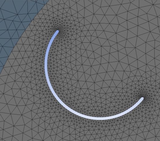
62 Figure 4-3: Mesh for Five Blade Turbine on Symmetry Plane Figure 4-4: Mesh for Six Blade Turbine on Symmetry Plane Figure 4-5: Mesh for Seven Blade Turbine on the Building on Symmetry Plane 52

63 Cm The torque variation as the turbine is rotating is shown for each turbine in Figure 4-6. Peaks in torque that correspond to the maximum torque producing rotational angle are clearly seen. There is an inversely proportional relation between the period between peaks in torque and the number of blades. The period between peaks is equivalent to the angular spacing between blades. Also, there is an inversely proportional relation between the amplitude of the oscillations and the number of blades. The oscillations are an important aspect of the turbine as they dictate the maximum and minimum torque produced by the turbine, which are related to the turbine s self-starting capabilities, a desirable attribute Rotation Angle (degree) 5 Blade d=0.22d x=0.25d 6 Blade d=0.22d x=0.25d 7 Blade d=0.22d x=0.25d 7 Blade d=0.22d Free Stream 2 Blade d=0.6d x=0 Figure 4-6: Instantaneous Cm vs Rotational Angle of the Last Cycle for each Turbine at TSR=0.4 Despite the more desirable self-starting capabilities with fewer blades, the larger oscillations lead to higher fatigue loading, and larger mechanical vibrations. There is a balance between high maximum torque values, low vibrations, and high power coefficient. To gain a better understanding of turbine behavior, it is important to consider the torque produced by each blade at any rotational angle individually because the maximum torque producing rotational angle of each blade does not correspond to that of the turbine. Most often, when one blade is at its best torque producing rotational angle, another blade is at its worst. 53

64 Cm Cm Rotational Angle (degree) Blade 1 Blade 2 Blade 3 Blade 4 Blade 5 Blade 6 Blade 7 Figure 4-7: Blade Moment Coefficient for Last Cycle of Seven Blade Turbine at TSR=0.6 Figure 4-7 shows that the seven blade turbine on the building has between 2-3 blades drawing power at any given rotational angle, however the ranges between which 3 blades are drawing power are very small Rotational Angle (degree) Blade 1 Blade 2 Blade 3 Blade 4 Blade 5 Blade 6 Blade 7 Figure 4-8: Blade Moment Coefficient for Last Cycle of Seven Blade Turbine Free Stream at TSR=0.39 When the seven blade turbine is placed in free stream flow (Figure 4-8), there are 4-5 blades drawing power at any given rotational angle, which explains the low moment coefficient of the free stream turbine in Figure

65 Cm Cm Rotational Angle (degree) Blade 1 Blade 2 Blade 3 Blade 4 Blade 5 Blade 6 Figure 4-9: Blade Moment Coefficient for Last Cycle of Six Blade Turbine at TSR=0.6 Figure 4-9 shows that when the six blade turbine is placed on the building, there are always 2 blades drawing power throughout its rotation Blade 1 Blade 2 Blade 3 Blade 4 Blade Rotational Angle (degree) Figure 4-10: Blade Moment Coefficient for Last Cycle of Five Blade Turbine at TSR=0.6 Interestingly, in the case where the five blade turbine is placed on the building, there are generally 1-2 blades drawing power, however, there are small rotational angle ranges in which all the blades produce power except one that is almost neutral (Figure 4-10). From the moment coefficients of each blade throughout their rotation (Figure 4-7 to Figure 4-10), it can be seen that when the turbine is placed on the building, regardless of the number of blades, there are almost always at least two blades drawing power instead of producing it. Although the moment coefficient is influenced by angular velocity and TSR, the conclusions apply across a range of TSRs. Moreover, as the number of blades increases, the maximum number of blades drawing power instead of producing it increases. This indicates that there is a range of rotational angles through which all blades perform poorly. 55

66 Cm Each blade shows the same moment coefficient profile, but shifted by a phase angle equivalent to the angular spacing between blades. In Figure 4-11, the difference between the five, six, and seven bladed turbine can be seen. When the blade is at 0 o, the blade receives very little oncoming flow as it is shielded by the building. Once the blade has passed this rotational angle, its concave side is gradually exposed to the accelerated flow, and it produces power in a drag based fashion. The moment characteristics are similar for all turbines when the blade travels between 0 o and 180 o because the influence of the other blades is minimal, however, in the range of 180 o to 360 o, the upstream blades play an important role. Interestingly, the five blade turbine shows a large peak around 240 o and a smaller peak around 330 o. These peaks can be attributed in part to lift. The upstream blades redirect flow in such a way that there is a significant acceleration of flow on the convex side of the blade leading to an important pressure drop. The six and seven blade turbines show similar lift effects around 270 o, but with a smaller magnitude. The smaller effect of lift in the turbines with more blades is attributed to the higher blockage of the turbine and the ease at which flow can pass through the turbine. This conclusion is interesting due to the fact that cup type turbines are usually perceived to be purely drag based devices, but the moment characteristics show that in the five blade case, lift can produce almost as much torque as drag, making the five blade turbine mostly drag based between degrees, and mostly lift based between degrees Blade d=0.22d x=0.25d 6 Blade d=0.22d x=0.25d 5 Blade d=0.22d x=0.25d Rotational Angle(degree) Figure 4-11: Moment Coefficient for Blade 1 throughout Rotation at TSR=0.4 56

67 Cp In Figure 4-12, the six bladed turbine is shown to have the highest power coefficient with a Cp of 0.17, but that the seven blade turbine performs very similarly. The importance of simulating a range of TSRs is clearly demonstrated. If the simulations only considered a TSR of 0.8, the conclusion would have been that the seven bladed turbine performed the best Blade d=0.6d x=0 7 Blade d=0.22d x=0.25d 7 Blade d=0.22d Free Stream 6 Blade d=0.22d x=0.25d 5 Blade d=0.22d x=0.25d TSR Figure 4-12: Cp vs TSR Summary The pressure contours and streamlines for five, six, and seven blade turbines are shown in Figure 4-13, Figure 4-14, and Figure The said figures are particularly useful to determine the effect and the interactions of the upstream blades on the downstream blades. Naturally, fewer blades increases the ease at which the flow can pass through the turbine. This leads to a larger region of accelerated flow inside the turbine, the effect of which can be seen in the torque characteristics of the blades throughout their rotation. In addition to the changes in velocity magnitude, the direction of flow inside the turbine becomes more horizontal as the number of blades increases. This is expected as the blades act similarly to guide vanes. In this case, more blades, hence less distance between each blade, leads to more significant redirection of the flow. 57

68 Figure 4-13: Pressure Contours and Streamlines on Symmetry Plane for Seven Blade Turbine at TSR=0.5 Figure 4-14: Pressure Contours and Streamlines on Symmetry Plane for Six Blade Turbine at TSR=0.5 Figure 4-15: Pressure Contours and Streamlines on Symmetry Plane for Five Blade Turbine at TSR=0.5 58

69 The pressure plots shown in Figure 4-13, Figure 4-14, and Figure 4-15 also provide information on how the front and back portions of the blades produce desirable or adverse torque from pressure differential between the concave and convex sides of the blades. For five, six, and seven blade turbines, there are rotational positions in which the front of the blade produces adverse torque while the back produces desirable torque, and vice-versa. 4.2 Blade Circumferential Length Optimization To evaluate whether the back and front portions of the blade provide a net benefit, the back of the blade will be circumferentially cut, then both the back and front will be cut. It was shown by Krishnan in [54] that for a shrouded seven blade cup type turbine, the optimal circumferential cut was 30 degrees. In all cases, the cut will be of 30 degrees from the original blade shape. To obtain a better understanding of the flow behavior, some parameters will be investigated simultaneously. The two best turbines from the blade number investigation will be used for further study. Although the six blade turbine showed the highest power coefficient with conventional blades, the circumferential length study could lead to a different conclusion, as the flow behavior is complex and multiple of the turbine s parameters are likely to be correlated. Both the six and seven blade turbines will be used as platforms for the blade circumferential length investigation. A range of TSRs are simulated such that the turbines behaviors are known for their operating range instead of a single operating point. The necessity for simulating a range of TSRs was shown in the previous section. The conventional blade, back cut blade (single cut), and back and front cut blade (double cut) are shown in Figure The hypothesis is that removing a portion of the blade will increase the lifting effect when the blade is between degrees while retaining the high torque produced when the blade is between degrees. Furthermore, from a practical point of view, each blade will require less material. 59

70 30 o 30 o 30 o Figure 4-16: Geometry for Conventional Blade (Left), Single Cut Blade (Middle), and Double Cut Blade (Right) The meshes around the turbine with the new blade geometries are shown in Figure 4-17 and Figure Note that the element sizing and solver properties have not changed. The only change is the blade s circumferential length, the blade s radius does not change. Figure 4-17: Mesh on Symmetry Plane for Seven Blade Turbine with Single Cut (Left) and Double Cut (Right) 60

71 Cm Cm Figure 4-18: Mesh on Symmetry Plane for Six Blade Turbine with Single Cut (Left) and Double Cut (Right) The modification to the blades leads to less periodic behavior of the overall turbine as seen in Figure 4-19 and Figure The instability could originate from the strength of the vortices present inside and around the turbine. Although the vortices are larger when using the full blades, the vortices produced when using the cut blades show greater velocity magnitude Rotational Angle (degree) 6 Blade 6 Blade Back-Cut 30 6 Blade Back & Front Cut 30 Figure 4-19: Moment Coefficient for Six Blade Turbine with different Blade Cuts for TSR= Rotational Angle (degree) 7 Blade 7 Blade Back-Cut 30 7 Blade Back & Front Cut 30 Figure 4-20: Moment Coefficient for Seven Blade Turbine with different Blade Cuts for TSR=0.4 61

72 It is also interesting to note that transitioning from the conventional blade to the double cut blade increases the amplitude of the overall turbine torque oscillations by around 50% for the six blade turbine (Figure 4-19), whereas the change for the seven blade turbine is negligible (Figure 4-20). When the back of the blades are cut, the flow inside the turbine shows not only a higher average velocity, but the regions of accelerated flow are larger (Figure 4-21 and Figure 4-22). This is expected as the blade become shorter and the blockage of the turbine decreases. Interestingly, the flow in the upstream portion of the turbine is not significantly changed in comparison with the uncut blade; however, the increased velocity of the flow passing through the turbine leads to a higher lifting effect for the blade between degrees. The angle at which the flow hits the concave side blades in the range of degrees is also better for producing drag based power. The result confirms the hypothesis; the turbine retains the torque produced by drag in the upstream portion of the turbine, while increasing the torque produced by lift in the downstream portion. Figure 4-21: Pressure Contours and Streamlines on Symmetry Plane for Seven 30 o Back Cut Blades at TSR=0.5 62

73 Figure 4-22: Pressure Contours and Streamlines on Symmetry Plane for Six 30 o Back Cut Blades at TSR=0.5 To further investigate the influence of circumferential length, the front of the blade will also be cut by 30 degrees. The study will again be performed for six and seven bladed turbines. As the diameter of the turbine is decreased when the front portion of the blade is cut, the power coefficients and moment coefficients are corrected to account for the slightly smaller area and outer radius of the turbine. As expected, when both the front and back of the blades are cut, the flow inside the turbine shows higher average velocity and larger regions of accelerated flow (Figure 4-23 and Figure 4-24). The double cut blades have a similar influence on the flow inside the turbine as the single cut blades. Despite this, in the case where the back and front of the blades are cut, the turbine gains torque produced by drag in the upstream portion of the turbine, while decreasing the torque produced by lift in the downstream portion of the turbine. This applies for both the six and seven bladed turbines. 63

74 Figure 4-23: Pressure Contours and Streamlines on Symmetry Plane for Six 30 o Back & Front Cut Blades at TSR=0.5 Figure 4-24: Pressure Contours and Streamlines on Symmetry Plane for Seven 30 o Back & Front Cut Blades at TSR=0.5 The effect of the circumferential cuts can also be seen in torque characteristics of the blade throughout their rotation (Figure 4-25). The lifting effect that was present between degrees is no longer shown; however, the blade produces more torque between degrees. To summarize, when the back of the blade is cut, the blade produces more torque between

75 Cm 360 degrees; when the back and front of the blade are cut, the blade produces more torque between degrees. 0.4 D C A B F E Blade 6 Blade Back-Cut 30 6 Blade Back & Front Cut Rotational Angle(degree) Figure 4-25: Moment Coefficient for Blade 1 throughout Rotation at TSR=0.4 for Different Blade Cuts for Six Blade Turbine A A A B F B F B F C E C C E E D D D Figure 4-26: Streamlines on Symmetry Plane for Six Blade Turbine with No Cut (Left), Single Cut (Middle), Double Cut (Right) The blade positions in Figure 4-26 correspond to the vertical lines illustrated in Figure For six bladed turbines, when the blade is in position A, the moment coefficient is similar for the uncut and single cut blades, but the double cut blades show around 50% larger moment coefficient. This can explained by the effect of the blade in position B. As the frontal area of the blade in position B is smaller relative to the other blade types, it allows more flow to reach the blade in position A. When the blade is in position F and E, the single cut blade shows a higher Cm than the other blade types. Furthermore, in position E, only the single cut blade produces power instead of drawing it. This can be attributed to the shorter back portion allowing more flow through, and the front of the 65

76 Cm blade capturing more flow and building more pressure on the concave side of the blade. As previously mentioned, blades in the upstream portion of the turbine (positions D, C, and B) show similar characteristics for all blade types as the interaction between blades is not shown in the performance of the upstream blades. 0.3 D C B A G F E Blade 7 Blade Back-Cut 30 7 Blade Back & Front Cut Rotational Angle(degree) Figure 4-27: Moment Coefficient for Blade 1 throughout Rotation at TSR=0.4 for Different Blade Cuts for Seven Blade Turbine B A G B A G B A G C F C F C F D E D E D E Figure 4-28: Streamlines on Symmetry Plane for Seven Blade Turbine at TSR=0.5 with No Cut (Left), Single Cut (Middle), Double Cut (Right) The blade positions in Figure 4-28 correspond to the vertical lines illustrated in Figure For seven bladed turbines, when the blade is in position A, the trend is the same as for six bladed turbines; the double cut blade shows around 50% higher Cm than the other blade types. In positions G and F, the single cut blade perform the best for the same reason as for the single cut blade used in the six blade turbine. In position E, none of the blade types produce useful torque, but the double cut blade shows least adverse torque. 66