Op-Amp Circuits: Part 3

Transcription

1 Op-Amp Circuits: Part 3 M. B. Patil mbpatil@ee.iitb.ac.in Department of Electrical Engineering Indian Institute of Technology Bombay

2 Introduction to filters Consider v(t) = v (t) + v 2 (t) = V m sin t + V m2 sin 2 t. v v v t (msec) t (msec)

3 Introduction to filters Consider v(t) = v (t) + v 2 (t) = V m sin t + V m2 sin 2 t. v v 2 v v LPF v o = v t (msec) t (msec) A low-pass filter with a cut-off frequency < c < 2 will pass the low-frequency component v (t) and remove the high-frequency component v 2 (t).

4 Introduction to filters Consider v(t) = v (t) + v 2 (t) = V m sin t + V m2 sin 2 t. v v 2 v v LPF v o = v v HPF v o = v t (msec) t (msec) A low-pass filter with a cut-off frequency < c < 2 will pass the low-frequency component v (t) and remove the high-frequency component v 2 (t). A high-pass filter with a cut-off frequency < c < 2 will pass the high-frequency component v 2 (t) and remove the low-frequency component v (t).

5 Introduction to filters Consider v(t) = v (t) + v 2 (t) = V m sin t + V m2 sin 2 t. v v 2 v v LPF v o = v v HPF v o = v t (msec) t (msec) A low-pass filter with a cut-off frequency < c < 2 will pass the low-frequency component v (t) and remove the high-frequency component v 2 (t). A high-pass filter with a cut-off frequency < c < 2 will pass the high-frequency component v 2 (t) and remove the low-frequency component v (t). There are some other types of filters, as we will see.

6 Ideal low-pass filter v i (t) H(j) v o (t) H(j) c V o(j) = H(j) V i (j).

7 Ideal low-pass filter v i (t) H(j) v o (t) H(j) c Vi(j) LPF Vo(j) c c V o(j) = H(j) V i (j).

8 Ideal low-pass filter v i (t) H(j) v o (t) H(j) c Vi(j) LPF Vo(j) c c V o(j) = H(j) V i (j). All components with < c appear at the output without attenuation. All components with > c get eliminated. (Note that the ideal low-pass filter has H(j) =, i.e., H(j) = + j.)

9 Ideal filters Low pass H(j) c

10 Ideal filters Low pass High pass H(j) H(j) c c

11 Ideal filters Low pass High pass H(j) H(j) c c Band pass H(j) L H

12 Ideal filters Low pass High pass H(j) H(j) c c Band pass Band reject H(j) H(j) L H L H

13 Ideal low-pass filter: example v v 2 Filter transfer function Filter output v 3.5 H(j) v f (khz) t (msec) t (msec)

14 Ideal high-pass filter: example v v 2 Filter transfer function Filter output v 3.5 H(j) v f (khz) t (msec) t (msec)

15 Ideal band-pass filter: example v v 2 Filter transfer function Filter output v 3 H(j).5 v f (khz) t (msec) t (msec)

16 Ideal band-reject filter: example v v 2 Filter transfer function.5 Filter output v 3.5 H(j) v f (khz) t (msec) t (msec)

17 Practical filter circuits * In practical filter circuits, the ideal filter response is approximated with a suitable H(j) that can be obtained with circuit elements. For example, H(s) = a 5 s 5 + a 4 s 4 + a 3 s 3 + a 2 s 2 + a s + a represents a 5 th -order low-pass filter.

18 Practical filter circuits * In practical filter circuits, the ideal filter response is approximated with a suitable H(j) that can be obtained with circuit elements. For example, H(s) = a 5 s 5 + a 4 s 4 + a 3 s 3 + a 2 s 2 + a s + a represents a 5 th -order low-pass filter. * Some commonly used approximations (polynomials) are the Butterworth, Chebyshev, Bessel, and elliptic functions.

19 Practical filter circuits * In practical filter circuits, the ideal filter response is approximated with a suitable H(j) that can be obtained with circuit elements. For example, H(s) = a 5 s 5 + a 4 s 4 + a 3 s 3 + a 2 s 2 + a s + a represents a 5 th -order low-pass filter. * Some commonly used approximations (polynomials) are the Butterworth, Chebyshev, Bessel, and elliptic functions. * Coefficients for these filters are listed in filter handbooks. Also, programs for filter design are available on the internet.

20 Practical filters H Low pass Ideal c H Amax Practical A min c s H Ideal High pass c H Amax A min Practical s c

21 Practical filters H Low pass Ideal c H Amax Practical A min c s H Ideal High pass c H Amax A min Practical s c * A practical filter may exhibit a ripple. A max is called the maximum passband ripple, e.g., A max = db.

22 Practical filters H Low pass Ideal c H Amax Practical A min c s H Ideal High pass c H Amax A min Practical s c * A practical filter may exhibit a ripple. A max is called the maximum passband ripple, e.g., A max = db. * A min is the minimum attenuation to be provided by the filter, e.g., A min = 6 db.

23 Practical filters H Low pass Ideal c H Amax Practical A min c s H Ideal High pass c H Amax A min Practical s c * A practical filter may exhibit a ripple. A max is called the maximum passband ripple, e.g., A max = db. * A min is the minimum attenuation to be provided by the filter, e.g., A min = 6 db. * s: edge of the stop band.

24 Practical filters H Low pass Ideal c H Amax Practical A min c s H Ideal High pass c H Amax A min Practical s c * A practical filter may exhibit a ripple. A max is called the maximum passband ripple, e.g., A max = db. * A min is the minimum attenuation to be provided by the filter, e.g., A min = 6 db. * s: edge of the stop band. * s/ c (for a low-pass filter): selectivity factor, a measure of the sharpness of the filter.

25 Practical filters H Low pass Ideal c H Amax Practical A min c s H Ideal High pass c H Amax A min Practical s c * A practical filter may exhibit a ripple. A max is called the maximum passband ripple, e.g., A max = db. * A min is the minimum attenuation to be provided by the filter, e.g., A min = 6 db. * s: edge of the stop band. * s/ c (for a low-pass filter): selectivity factor, a measure of the sharpness of the filter. * c < < s: transition band.

26 Practical filters For a low-pass filter, H(s) =. n a i (s/ c) i i= Coefficients (a i ) for various types of filters are tabulated in handbooks. We now look at H(j) for two commonly used filters.

27 Practical filters For a low-pass filter, H(s) =. n a i (s/ c) i i= Coefficients (a i ) for various types of filters are tabulated in handbooks. We now look at H(j) for two commonly used filters. Butterworth filters: H(j) = + ɛ 2 (/. c) 2n

28 Practical filters For a low-pass filter, H(s) =. n a i (s/ c) i i= Coefficients (a i ) for various types of filters are tabulated in handbooks. We now look at H(j) for two commonly used filters. Butterworth filters: H(j) = + ɛ 2 (/. c) 2n Chebyshev filters: H(j) = + ɛ 2 Cn 2 (/ c) where C n(x) = cos [ n cos (x) ] for x, C n(x) = cosh [ n cosh (x) ] for x,

29 Practical filters For a low-pass filter, H(s) =. n a i (s/ c) i i= Coefficients (a i ) for various types of filters are tabulated in handbooks. We now look at H(j) for two commonly used filters. Butterworth filters: H(j) = + ɛ 2 (/. c) 2n Chebyshev filters: H(j) = + ɛ 2 Cn 2 (/ c) where C n(x) = cos [ n cos (x) ] for x, C n(x) = cosh [ n cosh (x) ] for x, H(s) for a high-pass filter can be obtained from H(s) of the corresponding low-pass filter by (s/ c) ( c/s).

30 Practical filters (low-pass) Butterworth filters: ǫ =.5 n= H n= 2 H (db) /c /c 2 3 Chebyshev filters: ǫ =.5 n= H 2 n= H (db) /c /c

31 Practical filters (high-pass) Butterworth filters: n= H n= ǫ =.5 H (db) /c.. /c Chebyshev filters: n= H n= ǫ = /c H (db) /c

32 Passive filter example Vs R Ω Vo C 5 µf

33 Passive filter example Vs R Ω Vo C 5 µf H(s) = (/sc) R + (/sc) = + (s/ ), with = /RC f = /2π = 38 Hz (Low pass filter)

34 Passive filter example Vs R Ω Vo C 5 µf H(s) = (/sc) R + (/sc) = + (s/ ), with = /RC f = /2π = 38 Hz (Low pass filter) 2 H (db) f (Hz) (SEQUEL file: ee rc ac 2.sqproj) 5

35 Passive filter example Vs R Ω L. mf Vo C 4 µf

36 Passive filter example Vs R Ω L. mf Vo C 4 µf H(s) = (sl) (/sc) R + (sl) (/sc) = s(l/r) + s(l/r) + s 2 LC with = / LC f = /2π = 7.96 khz (Band pass filter)

37 Passive filter example Vs R Ω L. mf Vo C 4 µf H(s) = (sl) (/sc) R + (sl) (/sc) = s(l/r) + s(l/r) + s 2 LC with = / LC f = /2π = 7.96 khz (Band pass filter) 2 H (db) f (Hz) (SEQUEL file: ee rlc 3.sqproj)

38 Op-amp filters ( Active filters) * Op-amp filters can be designed without using inductors. This is a significant advantage since inductors are bulky and expensive. Inductors also exhibit nonlinear behaviour (arising from the core properties) which is undesirable in a filter circuit.

39 Op-amp filters ( Active filters) * Op-amp filters can be designed without using inductors. This is a significant advantage since inductors are bulky and expensive. Inductors also exhibit nonlinear behaviour (arising from the core properties) which is undesirable in a filter circuit. * With op-amps, a filter circuit can be designed with a pass-band gain.

40 Op-amp filters ( Active filters) * Op-amp filters can be designed without using inductors. This is a significant advantage since inductors are bulky and expensive. Inductors also exhibit nonlinear behaviour (arising from the core properties) which is undesirable in a filter circuit. * With op-amps, a filter circuit can be designed with a pass-band gain. * Op-amp filters can be easily incorporated in an integrated circuit.

41 Op-amp filters ( Active filters) * Op-amp filters can be designed without using inductors. This is a significant advantage since inductors are bulky and expensive. Inductors also exhibit nonlinear behaviour (arising from the core properties) which is undesirable in a filter circuit. * With op-amps, a filter circuit can be designed with a pass-band gain. * Op-amp filters can be easily incorporated in an integrated circuit. * However, there are situations in which passive filters are still used. - high frequencies at which op-amps do not have sufficient gain - high power which op-amps cannot handle

42 Op-amp filters: example R 2 k C V s R k nf V o R L

43 Op-amp filters: example R 2 k C V s R k nf V o R L Op-amp filters are designed for op-amp operation in the linear region Our analysis of the inverting amplifier applies, and we get, V o = R 2 (/sc) R V s (V s and V o are phasors) H(s) = R 2 R + sr 2 C

44 Op-amp filters: example R 2 k C V s R k nf V o R L Op-amp filters are designed for op-amp operation in the linear region Our analysis of the inverting amplifier applies, and we get, V o = R 2 (/sc) R V s (V s and V o are phasors) H(s) = R 2 R + sr 2 C This is a low-pass filter, with = /R 2 C (i.e., f = /2π =.59 khz).

45 Op-amp filters: example R 2 k C 2 V s R k nf V o H (db) R L f (Hz) Op-amp filters are designed for op-amp operation in the linear region Our analysis of the inverting amplifier applies, and we get, V o = R 2 (/sc) R V s (V s and V o are phasors) H(s) = R 2 R + sr 2 C This is a low-pass filter, with = /R 2 C (i.e., f = /2π =.59 khz). 4 5

46 Op-amp filters: example R 2 k C 2 V s R k nf V o H (db) R L f (Hz) Op-amp filters are designed for op-amp operation in the linear region Our analysis of the inverting amplifier applies, and we get, V o = R 2 (/sc) R V s (V s and V o are phasors) H(s) = R 2 R + sr 2 C This is a low-pass filter, with = /R 2 C (i.e., f = /2π =.59 khz). 4 5 (SEQUEL file: ee op filter.sqproj)

47 Op-amp filters: example R 2 V s R C k nf k V o R L

48 Op-amp filters: example R 2 V s R C k nf k V o R L R 2 H(s) = R + (/sc) = sr 2C + sr C.

49 Op-amp filters: example R 2 V s R C k nf k V o R L R 2 H(s) = R + (/sc) = sr 2C + sr C. This is a high-pass filter, with = /R C (i.e., f = /2π =.59 khz).

50 Op-amp filters: example 2 R 2 V s R C k nf k R L V o H (db) f (Hz) R 2 H(s) = R + (/sc) = sr 2C + sr C. This is a high-pass filter, with = /R C (i.e., f = /2π =.59 khz). 4 5

51 Op-amp filters: example 2 R 2 V s R C k nf k R L V o H (db) f (Hz) R 2 H(s) = R + (/sc) = sr 2C + sr C. This is a high-pass filter, with = /R C (i.e., f = /2π =.59 khz). (SEQUEL file: ee op filter 2.sqproj) 4 5

52 Op-amp filters: example R 2 V s R C k.8 µf k C 2 8 pf V o R L

53 Op-amp filters: example R 2 V s R C k.8 µf k C 2 8 pf V o R L H(s) = R 2 (/sc 2 ) R + (/sc ) = R 2 R sr C ( + sr C )( + sr 2 C 2 ).

54 Op-amp filters: example R 2 V s R C k.8 µf k C 2 8 pf V o R L H(s) = R 2 (/sc 2 ) R + (/sc ) = R 2 R sr C ( + sr C )( + sr 2 C 2 ). This is a band-pass filter, with L = /R C and H = /R 2 C 2. f L = 2 Hz, f H = 2 khz.

55 Op-amp filters: example R 2 k C 2 2 V s R C k.8 µf 8 pf V o H (db) R L H(s) = R 2 (/sc 2 ) R + (/sc ) = R 2 R sr C ( + sr C )( + sr 2 C 2 ). This is a band-pass filter, with L = /R C and H = /R 2 C 2. f L = 2 Hz, f H = 2 khz f (Hz)

56 Op-amp filters: example R 2 k C 2 2 V s R C k.8 µf 8 pf V o H (db) R L H(s) = R 2 (/sc 2 ) R + (/sc ) = R 2 R sr C ( + sr C )( + sr 2 C 2 ). This is a band-pass filter, with L = /R C and H = /R 2 C 2. f L = 2 Hz, f H = 2 khz. (SEQUEL file: ee op filter 3.sqproj) f (Hz)

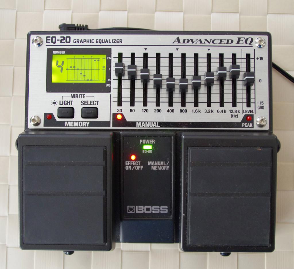
57 Graphic equalizer C a a 2 V s RA R2 C2 RB.7 a=.9 R3A R3B.5 RA = RB = 47 Ω.3 R3A = R3B = kω V o. R2 = kω C = nf R L C2 = nf f (Hz) (Ref.: S. Franco, "Design with Op Amps and analog ICs") H (db) 4 5

58 Graphic equalizer C a a 2 V s RA R2 C2 RB.7 a=.9 R3A R3B.5 RA = RB = 47 Ω.3 R3A = R3B = kω V o. R2 = kω C = nf R L C2 = nf f (Hz) (Ref.: S. Franco, "Design with Op Amps and analog ICs") H (db) 4 5 * Equalizers are implemented as arrays of narrow-band filters, each with an adjustable gain (attenuation) around a centre frequency.

59 Graphic equalizer C a a 2 V s RA R2 C2 RB.7 a=.9 R3A R3B.5 RA = RB = 47 Ω.3 R3A = R3B = kω V o. R2 = kω C = nf R L C2 = nf f (Hz) (Ref.: S. Franco, "Design with Op Amps and analog ICs") H (db) 4 5 * Equalizers are implemented as arrays of narrow-band filters, each with an adjustable gain (attenuation) around a centre frequency. * The circuit shown above represents one of the equalizer sections. (SEQUEL file: ee op filter 4.sqproj)

60

61 Sallen-Key filter example (2 nd order, low-pass) 4 C R R2 V s V V o C2 R L R = R2 = 5.8 kω RB C = C2 = nf RA RA = kω, RB = 7.8 kω (Ref.: S. Franco, "Design with Op Amps and analog ICs") H (db) f (Hz) 4 5

62 Sallen-Key filter example (2 nd order, low-pass) 4 V s R V R = R2 = 5.8 kω C = C2 = nf R2 C2 RA = kω, RB = 7.8 kω C RA RB (Ref.: S. Franco, "Design with Op Amps and analog ICs") V + = V = V o R A R A + R B V o/k. R L V o H (db) f (Hz) 4 5

63 Sallen-Key filter example (2 nd order, low-pass) 4 V s R V R = R2 = 5.8 kω C = C2 = nf R2 C2 RA = kω, RB = 7.8 kω C RA RB (Ref.: S. Franco, "Design with Op Amps and analog ICs") R A V + = V = V o V o/k. R A + R B (/sc 2) Also, V + = R 2 + (/sc 2) V = V. + sr 2C 2 R L V o H (db) f (Hz) 4 5

64 Sallen-Key filter example (2 nd order, low-pass) 4 V s R V R = R2 = 5.8 kω C = C2 = nf R2 C2 RA = kω, RB = 7.8 kω C RA RB (Ref.: S. Franco, "Design with Op Amps and analog ICs") R A V + = V = V o V o/k. R A + R B (/sc 2) Also, V + = R 2 + (/sc 2) V = V. + sr 2C 2 R L V o H (db) f (Hz) 4 5 KCL at V R (V s V ) + sc (V o V ) + R 2 (V + V ) =.

65 Sallen-Key filter example (2 nd order, low-pass) 4 V s R V R = R2 = 5.8 kω C = C2 = nf R2 C2 RA = kω, RB = 7.8 kω C RA RB (Ref.: S. Franco, "Design with Op Amps and analog ICs") R A V + = V = V o V o/k. R A + R B (/sc 2) Also, V + = R 2 + (/sc 2) V = V. + sr 2C 2 R L V o H (db) f (Hz) 4 5 KCL at V R (V s V ) + sc (V o V ) + R 2 (V + V ) =. Combining the above equations, H(s) = (SEQUEL file: ee op filter 5.sqproj) K + s [(R + R 2)C 2 + ( K)R C ] + s 2 R C R 2C 2.

66 Sixth-order Chebyshev low-pass filter (cascade design) 5. n n 62 n Vs.7 k.2 k 8.25 k 6.49 k 4.64 k 2.49 k 2.2 n 5 p 22 p R L Vo 2 (Ref.: S. Franco, "Design with Op Amps and analog ICs") SEQUEL file: ee_op_filter_6.sqproj H (db) f (Hz) 4 5

67 Third-order Chebyshev high-pass filter n 5.4 k 54 k k V s n n 54.9 k R L V o H (db) 2 4 (Ref.: S. Franco, "Design with Op Amps and analog ICs") 6 SEQUEL file: ee_op_filter_7.sqproj 8 f (Hz) 2 3

68 Band-pass filter example V s 5 k 5 k 5 k 5 k 7.4 n 5 k 7.4 n H (db) k 37 k V o (Ref.: J. M. Fiore, "Op Amps and linear ICs") f (Hz) SEQUEL file: ee_op_filter_8.sqproj

69 Notch filter example V s k k k k 265 n k 265 n k k 89 k k V o k (Ref.: J. M. Fiore, "Op Amps and linear ICs") SEQUEL file: ee_op_filter_9.sqproj H (db) 2 4 f (Hz) 2