Scottsdale Community College College Algebra Primary Authors Development Team

Transcription

1 Scottsdale Community College College Algebra Primary Authors Development Team

2 This tet is licensed under a Creative Commons Attribution-Share Alike 3.0 United States License. free to Share to Remi Attribution Share Alike Waiver. Other Rights Precalculus

3 Acknowledgements

4

5 How To Be Successful In This Course ASK: ASK FOR: FOR HELP: HELP

6 Table of Contents Chapter 1: Functions... 1 Chapter 2: Linear Functions Chapter 3: Polynomial and Rational Functions Chapter 4: Eponential and Logarithmic Functions

7 Chapter 5: Systems of Equations Chapter 6: Sequences and Series Solutions to Selected Eercises Inde

8

9 Chapter 1: Functions Section 1.1 Functions and Function Notation... 1 Section 1.2 Domain and Range Section 1.3 Rates of Change and Behavior of Graphs Section 1.4 Composition of Functions Section 1.5 Transformation of Functions Section 1.6 Inverse Functions Section 1.1 Functions and Function Notation What is a Function? The natural world is full of relationships between quantities that change. When we see these relationships, it is natural for us to ask If I know one quantity, can I then determine the other? This establishes the idea of an input quantity, or independent variable, and a corresponding output quantity, or dependent variable. From this we get the notion of a functional relationship in which the output can be determined from the input. For some quantities, like height and age, there are certainly relationships between these quantities. Given a specific person and any age, it is easy enough to determine their height, but if we tried to reverse that relationship and determine age from a given height, that would be problematic, since most people maintain the same height for many years. Function Function: A rule for a relationship between an input, or independent, quantity and an output, or dependent, quantity in which each input value uniquely determines one output value. We say the output is a function of the input. Eample 1 In the height and age eample above, is height a function of age? Is age a function of height? In the height and age eample above, it would be correct to say that height is a function of age, since each age uniquely determines a height. For eample, on my 18 th birthday, I had eactly one height of 69 inches. However, age is not a function of height, since one height input might correspond with more than one output age. For eample, for an input height of 70 inches, there is more than one output of age since I was 70 inches at the age of 20 and 21. This chapter is part of Precalculus: An Investigation of Functions Lippman & Rasmussen This material is licensed under a Creative Commons CC-BY-SA license.

10 2 Chapter 1 Eample 2 At a coffee shop, the menu consists of items and their prices. Is price a function of the item? Is the item a function of the price? We could say that price is a function of the item, since each input of an item has one output of a price corresponding to it. We could not say that item is a function of price, since two items might have the same price. Eample 3 In many classes the overall percentage you earn in the course corresponds to a decimal grade point. Is decimal grade a function of percentage? Is percentage a function of decimal grade? For any percentage earned, there would be a decimal grade associated, so we could say that the decimal grade is a function of percentage. That is, if you input the percentage, your output would be a decimal grade. Percentage may or may not be a function of decimal grade, depending upon the teacher s grading scheme. With some grading systems, there are a range of percentages that correspond to the same decimal grade. One-to-One Function Sometimes in a relationship each input corresponds to eactly one output, and every output corresponds to eactly one input. We call this kind of relationship a one-to-one function. From Eample 3, if each unique percentage corresponds to one unique decimal grade point and each unique decimal grade point corresponds to one unique percentage then it is a one-to-one function. Try it Now Let s consider bank account information. 1. Is your balance a function of your bank account number? (if you input a bank account number does it make sense that the output is your balance?) 2. Is your bank account number a function of your balance? (if you input a balance does it make sense that the output is your bank account number?) Function Notation To simplify writing out epressions and equations involving functions, a simplified notation is often used. We also use descriptive variables to help us remember the meaning of the quantities in the problem.

11 Section 1.1 Functions and Function Notation 3 Rather than write height is a function of age, we could use the descriptive variable h to represent height and we could use the descriptive variable a to represent age. height is a function of age if we name the function f we write h is f of a or more simply h = f(a) we could instead name the function h and write h(a) which is read h of a Remember we can use any variable to name the function; the notation h(a) shows us that h depends on a. The value a must be put into the function h to get a result. Be careful - the parentheses indicate that age is input into the function (Note: do not confuse these parentheses with multiplication!). Function Notation The notation output = f(input) defines a function named f. This would be read output is f of input Eample 4 Introduce function notation to represent a function that takes as input the name of a month, and gives as output the number of days in that month. The number of days in a month is a function of the name of the month, so if we name the function f, we could write days = f(month) or d = f(m). If we simply name the function d, we could write d(m) For eample, d(march) = 31, since March has 31 days. The notation d(m) reminds us that the number of days, d (the output) is dependent on the name of the month, m (the input) Eample 5 A function N = f(y) gives the number of police officers, N, in a town in year y. What does f(2005) = 300 tell us? When we read f(2005) = 300, we see the input quantity is 2005, which is a value for the input quantity of the function, the year (y). The output value is 300, the number of police officers (N), a value for the output quantity. Remember N=f(y). So this tells us that in the year 2005 there were 300 police officers in the town. Tables as Functions Functions can be represented in many ways: Words (as we did in the last few eamples), tables of values, graphs, or formulas. Represented as a table, we are presented with a list of input and output values.

12 4 Chapter 1 In some cases, these values represent everything we know about the relationship, while in other cases the table is simply providing us a few select values from a more complete relationship. Table 1: This table represents the input, number of the month (January = 1, February = 2, and so on) while the output is the number of days in that month. This represents everything we know about the months & days for a given year (that is not a leap year) (input) Month number, m (output) Days in month, D Table 2: The table below defines a function Q = g(n). Remember this notation tells us g is the name of the function that takes the input n and gives the output Q. n Q Table 3: This table represents the age of children in years and their corresponding heights. This represents just some of the data available for height and ages of children. (input) a, age in years (output) h, height inches Eample 6 Which of these tables define a function (if any)? Are any of them one-to-one? Input Output Input Output Input Output The first and second tables define functions. In both, each input corresponds to eactly one output. The third table does not define a function since the input value of 5 corresponds with two different output values. Only the first table is one-to-one; it is both a function, and each output corresponds to eactly one input. Although table 2 is a function, because each input corresponds to eactly one output, each output does not correspond to eactly one input so this function is not one-to-one. Table 3 is not even a function and so we don t even need to consider if it is a one-to-one function.

13 Section 1.1 Functions and Function Notation 5 Try it Now 3. If each percentage earned translated to one letter grade, would this be a function? Is it one-to-one? Solving and Evaluating Functions: When we work with functions, there are two typical things we do: evaluate and solve. Evaluating a function is what we do when we know an input, and use the function to determine the corresponding output. Evaluating will always produce one result, since each input of a function corresponds to eactly one output. Solving equations involving a function is what we do when we know an output, and use the function to determine the inputs that would produce that output. Solving a function could produce more than one solution, since different inputs can produce the same output. Eample 7 Using the table shown, where Q=g(n) a) Evaluate g(3) n Q Evaluating g(3) (read: g of 3 ) means that we need to determine the output value, Q, of the function g given the input value of n=3. Looking at the table, we see the output corresponding to n=3 is Q=7, allowing us to conclude g(3) = 7. b) Solve g(n) = 6 Solving g(n) = 6 means we need to determine what input values, n, produce an output value of 6. Looking at the table we see there are two solutions: n = 2 and n = 4. When we input 2 into the function g, our output is Q = 6 When we input 4 into the function g, our output is also Q = 6 Try it Now 4. Using the function in Eample 7, evaluate g(4) Graphs as Functions Oftentimes a graph of a relationship can be used to define a function. By convention, graphs are typically created with the input quantity along the horizontal ais and the output quantity along the vertical.

14 6 Chapter 1 The most common graph has y on the vertical ais and on the horizontal ais, and we say y is a function of, or y = f() when the function is named f. y Eample 8 Which of these graphs defines a function y=f()? Which of these graphs defines a oneto-one function? Looking at the three graphs above, the first two define a function y=f(), since for each input value along the horizontal ais there is eactly one output value corresponding, determined by the y-value of the graph. The 3 rd graph does not define a function y=f() since some input values, such as =2, correspond with more than one output value. Graph 1 is not a one-to-one function. For eample, the output value 3 has two corresponding input values, -2 and 2.3 Graph 2 is a one-to-one function; each input corresponds to eactly one output, and every output corresponds to eactly one input. Graph 3 is not even a function so there is no reason to even check to see if it is a one-toone function. Vertical Line Test The vertical line test is a handy way to think about whether a graph defines the vertical output as a function of the horizontal input. Imagine drawing vertical lines through the graph. If any vertical line would cross the graph more than once, then the graph does not define only one vertical output for each horizontal input.

15 Section 1.1 Functions and Function Notation 7 Horizontal Line Test Once you have determined that a graph defines a function, an easy way to determine if it is a one-to-one function is to use the horizontal line test. Draw horizontal lines through the graph. If any horizontal line crosses the graph more than once, then the graph does not define a one-to-one function. Evaluating a function using a graph requires taking the given input and using the graph to look up the corresponding output. Solving a function equation using a graph requires taking the given output and looking on the graph to determine the corresponding input. Eample 9 Given the graph below, a) Evaluate f(2) b) Solve f() = 4 a) To evaluate f(2), we find the input of =2 on the horizontal ais. Moving up to the graph gives the point (2, 1), giving an output of y=1. So f(2) = 1 b) To solve f() = 4, we find the value 4 on the vertical ais because if f() = 4 then 4 is the output. Moving horizontally across the graph gives two points with the output of 4: (-1,4) and (3,4). These give the two solutions to f() = 4: = -1 or = 3 This means f(-1)=4 and f(3)=4, or when the input is -1 or 3, the output is 4. Notice that while the graph in the previous eample is a function, getting two input values for the output value of 4 shows us that this function is not one-to-one. Try it Now 5. Using the graph from eample 9, solve f()=1. Formulas as Functions When possible, it is very convenient to define relationships using formulas. If it is possible to epress the output as a formula involving the input quantity, then we can define a function.

16 8 Chapter 1 Eample 10 Epress the relationship 2n + 6p = 12 as a function p = f(n) if possible. To epress the relationship in this form, we need to be able to write the relationship where p is a function of n, which means writing it as p = [something involving n]. 2n + 6p = 12 6p = 12-2n subtract 2n from both sides divide both sides by 6 and simplify 12 2n 12 2n 1 p 2 n Having rewritten the formula as p=, we can now epress p as a function: 1 p f( n) 2 n 3 It is important to note that not every relationship can be epressed as a function with a formula. Note the important feature of an equation written as a function is that the output value can be determined directly from the input by doing evaluations - no further solving is required. This allows the relationship to act as a magic bo that takes an input, processes it, and returns an output. Modern technology and computers rely on these functional relationships, since the evaluation of the function can be programmed into machines, whereas solving things is much more challenging. Eample 11 Epress the relationship y 2 2 If we try to solve for y in this equation: 2 2 y 1 y as a function y = f() if possible. We end up with two outputs corresponding to the same input, so this relationship cannot be represented as a single function y = f() As with tables and graphs, it is common to evaluate and solve functions involving formulas. Evaluating will require replacing the input variable in the formula with the value provided and calculating. Solving will require replacing the output variable in the formula with the value provided, and solving for the input(s) that would produce that output.

17 Section 1.1 Functions and Function Notation 9 Eample 12 Given the function a) Evaluate k(2) b) Solve k(t) = 1 kt 3 () t 2 a) To evaluate k(2), we plug in the input value 2 into the formula wherever we see the input variable t, then simplify 3 k(2) 2 2 k(2) 8 2 So k(2) = 10 b) To solve k(t) = 1, we set the formula for k(t) equal to 1, and solve for the input value that will produce that output 3 k(t) = 1 substitute the original formula kt () t 2 3 t 2 1 subtract 2 from each side 3 t 1 t 1 take the cube root of each side When solving an equation using formulas, you can check your answer by using your solution in the original equation to see if your calculated answer is correct. We want to know if kt () 1is true when t 1. 3 k( 1) ( 1) 2 = 1 2 = 1 which was the desired result. Eample 13 Given the function a) Evaluate h(4) b) Solve h(p) = 3 2 hp ( ) p 2p To evaluate h(4) we substitute the value 4 for the input variable p in the given function. 2 a) h(4) (4) 2(4) = = 24 b) h(p) = 3 Substitute the original function p p hp ( ) p 2p 2p 3 This is quadratic, so we can rearrange the equation to get it = 0 2p3 0 subtract 3 from each side 2 p 2p3 0 this is factorable, so we factor it ( p3)( p1) 0

18 10 Chapter 1 By the zero factor theorem since ( p3)( p1) 0, either ( p 3) 0 or ( p 1) 0 (or both of them equal 0) and so we solve both equations for p, finding p = -3 from the first equation and p = 1 from the second equation. This gives us the solution: h(p) = 3 when p = 1 or p = -3 We found two solutions in this case, which tells us this function is not one-to-one. Try it Now 6. Given the function gm ( ) m 4 a. Evaluate g(5) b. Solve g(m) = 2 Basic Toolkit Functions In this tet, we will be eploring functions the shapes of their graphs, their unique features, their equations, and how to solve problems with them. When learning to read, we start with the alphabet. When learning to do arithmetic, we start with numbers. When working with functions, it is similarly helpful to have a base set of elements to build from. We call these our toolkit of functions a set of basic named functions for which we know the graph, equation, and special features. For these definitions we will use as the input variable and f() as the output variable. Toolkit Functions Linear Constant: f( ) Identity: f( ) c, where c is a constant (number) Absolute Value: f ( ) Power Quadratic: f ( ) Cubic: 3 f ( ) Reciprocal: 1 f( ) Reciprocal squared: 1 f( ) 2 Square root: 2 f( ) Cube root: f( ) 3 2

19 Section 1.1 Functions and Function Notation 11 You will see these toolkit functions, combinations of toolkit functions, their graphs and their transformations frequently throughout this book. In order to successfully follow along later in the book, it will be very helpful if you can recognize these toolkit functions and their features quickly by name, equation, graph and basic table values. Not every important equation can be written as y = f(). An eample of this is the equation of a circle. Recall the distance formula for the distance between two points: 2 y 2 dist y1 A circle with radius r with center at (h, k) can be described as all points (, y) a distance r h 2 y k of r from the center, so using the distance formula, 2, giving Equation of a circle A circle with radius r with center (h, k) has equation 2 2 r 2 h y k Graphs of the Toolkit Functions Constant Function: f( ) 2 Identity: f( ) Absolute Value: f ( ) Quadratic: 2 f ( ) Cubic: 3 f ( ) Square root: f( )

20 12 Chapter 1 3 Cube root: f( ) Reciprocal: f( ) 1 1 Reciprocal squared: f( ) 2 Important Topics of this Section Definition of a function Input (independent variable) Output (dependent variable) Definition of a one-to-one function Function notation Descriptive variables Functions in words, tables, graphs & formulas Vertical line test Horizontal line test Evaluating a function at a specific input value Solving a function given a specific output value Toolkit Functions Try it Now Answers 1. Yes 2. No 3. Yes it s a function; No, it s not one-to-one 4. Q=g(4)=6 5. = 0 or = 2 6. a. g(5)=1 b. m = 8

21 Section 1.1 Functions and Function Notation 13 Section 1.1 Eercises 1. The amount of garbage, G, produced by a city with population p is given by G f( p). G is measured in tons per week, and p is measured in thousands of people. a. The town of Tola has a population of 40,000 and produces 13 tons of garbage each week. Epress this information in terms of the function f. b. Eplain the meaning of the statement f The number of cubic yards of dirt, D, needed to cover a garden with area a square feet is given by D g( a). a. A garden with area 5000 ft 2 requires 50 cubic yards of dirt. Epress this information in terms of the function g. b. Eplain the meaning of the statement g Let f() t be the number of ducks in a lake t years after Eplain the meaning of each statement: a. f 5 30 b. f Let ht () be the height above ground, in feet, of a rocket t seconds after launching. Eplain the meaning of each statement: a. h b. h Select all of the following graphs which represent y as a function of. a b c d e f

22 14 Chapter 1 6. Select all of the following graphs which represent y as a function of. a b c d e f 7. Select all of the following tables which represent y as a function of. a b c y y y Select all of the following tables which represent y as a function of. a b c y y y Select all of the following tables which represent y as a function of. a. y b. y c. y d. y Select all of the following tables which represent y as a function of. a. y b. y c. y d. y

23 Section 1.1 Functions and Function Notation Select all of the following tables which represent y as a function of and are one-toone. a y b y c y Select all of the following tables which represent y as a function of and are one-toone. a y b y c y Select all of the following graphs which are one-to-one functions. a. b. c. d. e. f. 14. Select all of the following graphs which are one-to-one functions. a b c d e f

24 16 Chapter 1 Given each function f( ) graphed, evaluate f (1) and f (3) Given the function g ( ) graphed here, a. Evaluate g (2) b. Solve g Given the function f( ) graphed here. a. Evaluate f 4 b. Solve f( ) Based on the table below, a. Evaluate f (3) b. Solve f( ) f( ) Based on the table below, a. Evaluate f (8) b. Solve f( ) f( ) For each of the following functions, evaluate: f 2, f ( 1), f (0), f (1), and f (2) 21. f f f f f f f f f 2( 3) 30. f f 32. f 1 2 f 33. f

25 Section 1.1 Functions and Function Notation 17 f 8 4. Compute the following: a. f( 1) f(1) b. f( 1) f(1) 35. Suppose 2 f 3. Compute the following: a. f( 2) f(4) b. f( 2) f(4) 36. Suppose Let f t 3t 5 a. Evaluate f (0) b. Solve f t Let gp6 2p a. Evaluate g (0) b. Solve gp Match each function name with its equation. a. y i. Cube root b. 3 y ii. Reciprocal 3 c. y iii. Linear iv. Square Root 1 d. y v. Absolute Value vi. Quadratic 2 e. y vii. Reciprocal Squared f. y viii. Cubic g. y h. 1 y Match each graph with its equation. a. y 3 b. y 3 c. y 1 d. y 2 e. y f. y g. y 1 h. y 2 i. ii. iii. iv. v. vi. vii. viii.

26 18 Chapter Match each table with its equation. 2 a. y i. In Out b. y c. y 0 _ d. y 1/ 1 1 e. y f. y ii. In Out iii. In Out iv. In Out v. In Out -2 _ -1 _ vi. In Out Match each equation with its table a. Quadratic i. In Out b. Absolute Value c. Square Root -1-1 d. Linear 0 _ e. Cubic 1 1 f. Reciprocal ii. In Out iii. In Out iv. In Out v. In Out -2 _ -1 _ vi. In Out Write the equation of the circle centered at (3, 9 ) with radius Write the equation of the circle centered at (9, 8 ) with radius Sketch a reasonable graph for each of the following functions. [UW] a. Height of a person depending on age. b. Height of the top of your head as you jump on a pogo stick for 5 seconds. c. The amount of postage you must put on a first class letter, depending on the weight of the letter.

27 Section 1.1 Functions and Function Notation Sketch a reasonable graph for each of the following functions. [UW] a. Distance of your big toe from the ground as you ride your bike for 10 seconds. b. Your height above the water level in a swimming pool after you dive off the high board. c. The percentage of dates and names you ll remember for a history test, depending on the time you study. 47. Using the graph shown, a. Evaluate f() c b. Solve f p c. Suppose f b z. Find f() z d. What are the coordinates of points L and K? a b K t r p L c f() 48. Dave leaves his office in Padelford Hall on his way to teach in Gould Hall. Below are several different scenarios. In each case, sketch a plausible (reasonable) graph of the function s = d(t) which keeps track of Dave s distance s from Padelford Hall at time t. Take distance units to be feet and time units to be minutes. Assume Dave s path to Gould Hall is long a straight line which is 2400 feet long. [UW] a. Dave leaves Padelford Hall and walks at a constant spend until he reaches Gould Hall 10 minutes later. b. Dave leaves Padelford Hall and walks at a constant speed. It takes him 6 minutes to reach the half-way point. Then he gets confused and stops for 1 minute. He then continues on to Gould Hall at the same constant speed he had when he originally left Padelford Hall. c. Dave leaves Padelford Hall and walks at a constant speed. It takes him 6 minutes to reach the half-way point. Then he gets confused and stops for 1 minute to figure out where he is. Dave then continues on to Gould Hall at twice the constant speed he had when he originally left Padelford Hall.

28 20 Chapter 1 d. Dave leaves Padelford Hall and walks at a constant speed. It takes him 6 minutes to reach the half-way point. Then he gets confused and stops for 1 minute to figure out where he is. Dave is totally lost, so he simply heads back to his office, walking the same constant speed he had when he originally left Padelford Hall. e. Dave leaves Padelford heading for Gould Hall at the same instant Angela leaves Gould Hall heading for Padelford Hall. Both walk at a constant speed, but Angela walks twice as fast as Dave. Indicate a plot of distance from Padelford vs. time for the both Angela and Dave. f. Suppose you want to sketch the graph of a new function s = g(t) that keeps track of Dave s distance s from Gould Hall at time t. How would your graphs change in (a)-(e)?

29 Section 1.2 Domain and Range 21 Section 1.2 Domain and Range One of our main goals in mathematics is to model the real world with mathematical functions. In doing so, it is important to keep in mind the limitations of those models we create. This table shows a relationship between circumference and height of a tree as it grows. Circumference, c Height, h While there is a strong relationship between the two, it would certainly be ridiculous to talk about a tree with a circumference of -3 feet, or a height of 3000 feet. When we identify limitations on the inputs and outputs of a function, we are determining the domain and range of the function. Domain and Range Domain: The set of possible input values to a function Range: The set of possible output values of a function Eample 1 Using the tree table above, determine a reasonable domain and range. We could combine the data provided with our own eperiences and reason to approimate the domain and range of the function h = f(c). For the domain, possible values for the input circumference c, it doesn t make sense to have negative values, so c > 0. We could make an educated guess at a maimum reasonable value, or look up that the maimum circumference measured is about 119 feet 1. With this information we would say a reasonable domain is 0 c 119feet. Similarly for the range, it doesn t make sense to have negative heights, and the maimum height of a tree could be looked up to be 379 feet, so a reasonable range is 0 h 379 feet. Eample 2 When sending a letter through the United States Postal Service, the price depends upon the weight of the letter 2, as shown in the table below. Determine the domain and range. 1 retrieved July 19, retrieved July 19, 2010

30 22 Chapter 1 Letters Weight not Over Price 1 ounce $ ounces $ ounces $ ounces $0.95 Suppose we notate Weight by w and Price by p, and set up a function named P, where Price, p is a function of Weight, w. p = P(w). Since acceptable weights are 3.5 ounces or less, and negative weights don t make sense, the domain would be 0w 3.5. Technically 0 could be included in the domain, but logically it would mean we are mailing nothing, so it doesn t hurt to leave it out. Since possible prices are from a limited set of values, we can only define the range of this function by listing the possible values. The range is p = $0.44, $0.61, $0.78, or $0.95. Try it Now 1. The population of a small town in the year 1960 was 100 people. Since then the population has grown to 1400 people reported during the 2010 census. Choose descriptive variables for your input and output and use interval notation to write the domain and range. Notation In the previous eamples, we used inequalities to describe the domain and range of the functions. This is one way to describe intervals of input and output values, but is not the only way. Let us take a moment to discuss notation for domain and range. Using inequalities, such as 0 c 163, 0w 3.5, and 0 h 379 imply that we are interested in all values between the low and high values, including the high values in these eamples. However, occasionally we are interested in a specific list of numbers like the range for the price to send letters, p = $0.44, $0.61, $0.78, or $0.95. These numbers represent a set of specific values: {0.44, 0.61, 0.78, 0.95} Representing values as a set, or giving instructions on how a set is built, leads us to another type of notation to describe the domain and range. Suppose we want to describe the values for a variable that are 10 or greater, but less than 30. In inequalities, we would write

31 Section 1.2 Domain and Range 23 When describing domains and ranges, we sometimes etend this into set-builder notation, which would look like this: The curly brackets {} are read as the set of, and the vertical bar is read as such that, so altogether we would read as the set of -values such that 10 is less than or equal to and is less than 30. When describing ranges in set-builder notation, we could similarly write something like f( ) 0 f( ) 100, or if the output had its own variable, we could use it. So for our tree height eample above, we could write for the range h 0 h 379. In set-builder notation, if a domain or range is not limited, we could write t t is a real number, or t t, read as the set of t-values such that t is an element of the set of real numbers. A more compact alternative to set-builder notation is interval notation, in which intervals of values are referred to by the starting and ending values. Curved parentheses are used for strictly less than, and square brackets are used for less than or equal to. Since infinity is not a number, we can t include it in the interval, so we always use curved parentheses with and -. The table below will help you see how inequalities correspond to set-builder notation and interval notation: Inequality Set Builder Notation Interval notation 5 h 10 h 5h 10 (5, 10] 5h 10 h 5h 10 [5, 10) 5h 10 h 5h 10 (5, 10) h h 10 h h 10 [10, ) all real numbers h h (, ) h h (,10) To combine two intervals together, using inequalities or set-builder notation we can use the word or. In interval notation, we use the union symbol,, to combine two unconnected intervals together. Eample 3 Describe the intervals of values shown on the line graph below using set builder and interval notations.

32 24 Chapter 1 To describe the values,, that lie in the intervals shown above we would say, is a real number greater than or equal to 1 and less than or equal to 3, or a real number greater than 5. As an inequality it is: 13or 5 In set builder notation: 13or 5 In interval notation: [1, 3] (5, ) Remember when writing or reading interval notation: Using a square bracket [ means the start value is included in the set Using a parenthesis ( means the start value is not included in the set Try it Now 2. Given the following interval, write its meaning in words, set builder notation, and interval notation. Domain and Range from Graphs We can also talk about domain and range based on graphs. Since domain refers to the set of possible input values, the domain of a graph consists of all the input values shown on the graph. Remember that input values are almost always shown along the horizontal ais of the graph. Likewise, since range is the set of possible output values, the range of a graph we can see from the possible values along the vertical ais of the graph. Be careful if the graph continues beyond the window on which we can see the graph, the domain and range might be larger than the values we can see.

33 Section 1.2 Domain and Range 25 Eample 4 Determine the domain and range of the graph below. In the graph above 3, the input quantity along the horizontal ais appears to be year, which we could notate with the variable y. The output is thousands of barrels of oil per day, which we might notate with the variable b, for barrels. The graph would likely continue to the left and right beyond what is shown, but based on the portion of the graph that is shown to us, we can determine the domain is 1975 y 2008, and the range is approimately180 b In interval notation, the domain would be [1975, 2008] and the range would be about [180, 2010]. For the range, we have to approimate the smallest and largest outputs since they don t fall eactly on the grid lines. Remember that, as in the previous eample, and y are not always the input and output variables. Using descriptive variables is an important tool to remembering the contet of the problem. 3 CC-BY-SA, July 19, 2010

34 26 Chapter 1 Try it Now 3. Given the graph below write the domain and range in interval notation Domains and Ranges of the Toolkit functions We will now return to our set of toolkit functions to note the domain and range of each. Constant Function: f( ) c The domain here is not restricted; can be anything. When this is the case we say the domain is all real numbers. The outputs are limited to the constant value of the function. Domain: (, ) Range: [c] Since there is only one output value, we list it by itself in square brackets. Identity Function: f( ) Domain: (, ) Range: (, ) 2 Quadratic Function: f( ) Domain: (, ) Range: [0, ) Multiplying a negative or positive number by itself can only yield a positive output. Cubic Function: f( ) Domain: (, ) Range: (, ) 3

35 Section 1.2 Domain and Range 27 1 Reciprocal: f( ) Domain: (,0) (0, ) Range: (,0) (0, ) We cannot divide by 0 so we must eclude 0 from the domain. One divide by any value can never be 0, so the range will not include 0. 1 Reciprocal squared: f( ) 2 Domain: (,0) (0, ) Range: (0, ) We cannot divide by 0 so we must eclude 0 from the domain. 3 Cube Root: f( ) Domain: (, ) Range: (, ) 2 Square Root: f( ), commonly just written as, f( ) Domain: [0, ) Range: [0, ) When dealing with the set of real numbers we cannot take the square root of a negative number so the domain is limited to 0 or greater. Absolute Value Function: f( ) Domain: (, ) Range: [0, ) Since absolute value is defined as a distance from 0, the output can only be greater than or equal to 0. Eample 4.5 Find the domain of each function: a) f ( ) 2 4 b) 3 g( ) 6 3 a) Since we cannot take the square root of a negative number, we need the inside of the square root to be non-negative. 4 0 when 4. The domain of f() is [ 4, ). b) We cannot divide by zero, so we need the denominator to be non-zero when = 2, so we must eclude 2 from the domain. The domain of g() is (,2) (2, ).

36 28 Chapter 1 Piecewise Functions In the toolkit functions we introduced the absolute value function f( ). With a domain of all real numbers and a range of values greater than or equal to 0, the absolute value can be defined as the magnitude or modulus of a number, a real number value regardless of sign, the size of the number, or the distance from 0 on the number line. All of these definitions require the output to be greater than or equal to 0. If we input 0, or a positive value the output is unchanged f( ) if 0 If we input a negative value the sign must change from negative to positive. f( ) if 0 since multiplying a negative value by -1 makes it positive. Since this requires two different processes or pieces, the absolute value function is often called the most basic piecewise defined function. Piecewise Function A piecewise function is a function in which the formula used depends upon the domain the input lies in. We notate this idea like: formula 1 if domain to use formula 1 f( ) formula 2 if domain to use formula 2 formula 3 if domain to use formula 3 Eample 5 A museum charges $5 per person for a guided tour with a group of 1 to 9 people, or a fied $50 fee for 10 or more people in the group. Set up a function relating the number of people, n, to the cost, C. To set up this function, two different formulas would be needed. C = 5n would work for n values under 10, and C = 50 would work for values of n ten or greater. Notating this: 5n if 0n10 Cn ( ) 50 if n 10 Eample 6 A cell phone company uses the function below to determine the cost, C, in dollars for g gigabytes of data transfer. 25 if 0 g 2 Cg ( ) 25 10( g2) if g 2

37 Section 1.2 Domain and Range 29 Find the cost of using 1.5 gigabytes of data, and the cost of using 4 gigabytes of data. To find the cost of using 1.5 gigabytes of data, C(1.5), we first look to see which piece of domain our input falls in. Since 1.5 is less than 2, we use the first formula, giving C(1.5) = $25. The find the cost of using 4 gigabytes of data, C(4), we see that our input of 4 is greater than 2, so we ll use the second formula. C(4) = (4-2) = $45. Eample 7 Sketch a graph of the function 2 if 1 f( ) 3 if 1 2 if 2 Since each of the component functions are from our library of Toolkit functions, we know their shapes. We can imagine graphing each function, then limiting the graph to the indicated domain. At the endpoints of the domain, we put open circles to indicate where the endpoint is not included, due to a strictly-less-than inequality, and a closed circle where the endpoint is included, due to a less-than-or-equal-to inequality. Now that we have each piece individually, we combine them onto the same graph:

38 30 Chapter 1 Try it Now 4. At Pierce College during the school year tuition rates for in-state residents were $89.50 per credit for the first 10 credits, $33 per credit for credits 11-18, and for over 18 credits the rate is $73 per credit 4. Write a piecewise defined function for the total tuition, T, at Pierce College during as a function of the number of credits taken, c. Be sure to consider a reasonable domain and range. Important Topics of this Section Definition of domain Definition of range Inequalities Interval notation Set builder notation Domain and Range from graphs Domain and Range of toolkit functions Piecewise defined functions Try it Now Answers 1. Domain; y = years [1960,2010] ; Range, p = population, [100,1400] 2. a. Values that are less than or equal to -2, or values that are greater than or equal to - 1 and less than 3 2or 1 3 b. c. (, 2] [ 1,3) 3. Domain; y=years, [1952,2002] ; Range, p=population in millions, [40,88] 89.5c if c T ( c) ( c 10) if 10 c 18 Tuition, T, as a function of credits, c ( c 18) if c 18 Reasonable domain should be whole numbers 0 to (answers may vary), e.g. [0,23] Reasonable range should be $0 (answers may vary), e.g. [0,1524] 4 retrieved August 6, 2010

39 Section 1.2 Domain and Range 31 Section 1.2 Eercises Write the domain and range of the function using interval notation Write the domain and range of each graph as an inequality Suppose that you are holding your toy submarine under the water. You release it and it begins to ascend. The graph models the depth of the submarine as a function of time, stopping once the sub surfaces. What is the domain and range of the function in the graph? 5. 6.

40 32 Chapter 1 Find the domain of each function 7. f f f f f 12. f f f f f f f Given each function, evaluate: f ( 1), f (0), f (2), f (4) 73 if 0 49 if f 20. f 76 if if f if if 2 5 if 0 f 3 if if f if 1 1 if 1 3 if 1 0 f 4 if if 3

41 Section 1.2 Domain and Range 33 Write a formula for the piecewise function graphed below Sketch a graph of each piecewise function 31. f if 2 5 if f 4 if 0 if f if 0 2 if 0 3 if 2 f 1 if if 1 f if 1 if 1 3 if 2 f 1 if if 2

42 34 Chapter 1 Section 1.3 Rates of Change and Behavior of Graphs Since functions represent how an output quantity varies with an input quantity, it is natural to ask about the rate at which the values of the function are changing. For eample, the function C(t) below gives the average cost, in dollars, of a gallon of gasoline t years after t C(t) If we were interested in how the gas prices had changed between 2002 and 2009, we could compute that the cost per gallon had increased from $1.47 to $2.14, an increase of $0.67. While this is interesting, it might be more useful to look at how much the price changed per year. You are probably noticing that the price didn t change the same amount each year, so we would be finding the average rate of change over a specified amount of time. The gas price increased by $0.67 from 2002 to 2009, over 7 years, for an average of $ dollars per year. On average, the price of gas increased by about 9.6 7years cents each year. Rate of Change A rate of change describes how the output quantity changes in relation to the input quantity. The units on a rate of change are output units per input units Some other eamples of rates of change would be quantities like: A population of rats increases by 40 rats per week A barista earns $9 per hour (dollars per hour) A farmer plants 60,000 onions per acre A car can drive 27 miles per gallon A population of grey whales decreases by 8 whales per year The amount of money in your college account decreases by $4,000 per quarter Average Rate of Change The average rate of change between two input values is the total change of the function values (output values) divided by the change in the input values. Change of Output y y2 y1 Average rate of change = = Change of Input 2 1

43 Section 1.3 Rates of Change and Behavior of Graphs 35 Eample 1 Using the cost-of-gas function from earlier, find the average rate of change between 2007 and 2009 From the table, in 2007 the cost of gas was $2.64. In 2009 the cost was $2.14. The input (years) has changed by 2. The output has changed by $ $2.64 = $0.50 The average rate of change is then = dollars per year 2years Try it Now 1. Using the same cost-of-gas function, find the average rate of change between 2003 and 2008 Notice that in the last eample the change of output was negative since the output value of the function had decreased. Correspondingly, the average rate of change is negative. Eample 2 Given the function g(t) shown here, find the average rate of change on the interval [0, 3]. At t = 0, the graph shows g ( 0) 1 At t = 3, the graph shows g ( 3) 4 The output has changed by 3 while the input has changed by 3, giving an average rate of change of: Eample 3 On a road trip, after picking up your friend who lives 10 miles away, you decide to record your distance from home over time. Find your average speed over the first 6 hours. t (hours) D(t) (miles) Here, your average speed is the average rate of change. You traveled 282 miles in 6 hours, for an average speed of = 47 miles per hour 6 0 6

44 36 Chapter 1 We can more formally state the average rate of change calculation using function notation. Average Rate of Change using Function Notation Given a function f(), the average rate of change on the interval [a, b] is Change of Output f ( b) f ( a) Average rate of change = Change of Input b a Eample 4 Compute the average rate of change of 1 f ( ) 2 on the interval [2, 4] We can start by computing the function values at each endpoint of the interval f (2) f (4) Now computing the average rate of change 63 7 f (4) f (2) Average rate of change = Try it Now 2. Find the average rate of change of f ( ) 2 on the interval [1, 9] Eample 5 The magnetic force F, measured in Newtons, between two magnets is related to the 2 distance between the magnets d, in centimeters, by the formula F( d). Find the 2 d average rate of change of force if the distance between the magnets is increased from 2 cm to 6 cm. 2 We are computing the average rate of change of F( d) on the interval [2, 6] 2 d F(6) F(2) Average rate of change = Evaluating the function 6 2

45 Section 1.3 Rates of Change and Behavior of Graphs 37 F(6) F(2) = Simplifying Combining the numerator terms Simplifying further 4 1 Newtons per centimeter 9 This tells us the magnetic force decreases, on average, by 1/9 Newtons per centimeter over this interval. Eample 6 2 Find the average rate of change of g( t) t 3t 1on the interval [ 0, a ]. Your answer will be an epression involving a. Using the average rate of change formula g( a) g(0) a ( a 3a 1) (0 3(0) 1) a 0 2 a 3a 11 a a ( a 3) a a 3 Evaluating the function Simplifying Simplifying further, and factoring Cancelling the common factor a This result tells us the average rate of change between t = 0 and any other point t = a. For eample, on the interval [0, 5], the average rate of change would be 5+3 = 8. Try it Now 3. Find the average rate of change of f ( ) 3 2 on the interval [ a, a h].

46 38 Chapter 1 Graphical Behavior of Functions As part of eploring how functions change, it is interesting to eplore the graphical behavior of functions. Increasing/Decreasing A function is increasing on an interval if the function values increase as the inputs increase. More formally, a function is increasing if f(b) > f(a) for any two input values a and b in the interval with b>a. The average rate of change of an increasing function is positive. A function is decreasing on an interval if the function values decrease as the inputs increase. More formally, a function is decreasing if f(b) < f(a) for any two input values a and b in the interval with b>a. The average rate of change of a decreasing function is negative. Eample 7 Given the function p(t) graphed here, on what intervals does the function appear to be increasing? The function appears to be increasing from t = 1 to t = 3, and from t = 4 on. In interval notation, we would say the function appears to be increasing on the interval (1, 3) and the interval ( 4, ) Notice in the last eample that we used open intervals (intervals that don t include the endpoints) since the function is neither increasing nor decreasing at t = 1, 3, or 4. Local Etrema A point where a function changes from increasing to decreasing is called a local maimum. A point where a function changes from decreasing to increasing is called a local minimum. Together, local maima and minima are called the local etrema, or local etreme values, of the function.

47 Section 1.3 Rates of Change and Behavior of Graphs 39 Eample 8 Using the cost of gasoline function from the beginning of the section, find an interval on which the function appears to be decreasing. Estimate any local etrema using the table. t C(t) It appears that the cost of gas increased from t = 2 to t = 8. It appears the cost of gas decreased from t = 8 to t = 9, so the function appears to be decreasing on the interval (8, 9). Since the function appears to change from increasing to decreasing at t = 8, there is local maimum at t = 8. Eample 9 Use a graph to estimate the local etrema of the function f ( ) determine the intervals on which the function is increasing. 2. Use these to 3 Using technology to graph the function, it appears there is a local minimum somewhere between = 2 and =3, and a symmetric local maimum somewhere between = -3 and = -2. Most graphing calculators and graphing utilities can estimate the location of maima and minima. Below are screen images from two different technologies, showing the estimate for the local maimum and minimum. Based on these estimates, the function is increasing on the intervals (, 2.449) and ( 2.449, ). Notice that while we epect the etrema to be symmetric, the two different technologies agree only up to 4 decimals due to the differing approimation algorithms used by each.

48 40 Chapter 1 Try it Now Use a graph of the function f ( ) to estimate the local etrema of the function. Use these to determine the intervals on which the function is increasing and decreasing. Concavity The total sales, in thousands of dollars, for two companies over 4 weeks are shown. Company A Company B As you can see, the sales for each company are increasing, but they are increasing in very different ways. To describe the difference in behavior, we can investigate how the average rate of change varies over different intervals. Using tables of values, Company A Week Sales Rate of Change Company B Week Sales Rate of Change From the tables, we can see that the rate of change for company A is decreasing, while the rate of change for company B is increasing.

49 Section 1.3 Rates of Change and Behavior of Graphs 41 Larger increase Smaller increase Larger increase Smaller increase When the rate of change is getting smaller, as with Company A, we say the function is concave down. When the rate of change is getting larger, as with Company B, we say the function is concave up. Concavity A function is concave up if the rate of change is increasing. A function is concave down if the rate of change is decreasing. A point where a function changes from concave up to concave down or vice versa is called an inflection point. Eample 10 An object is thrown from the top of a building. The object s height in feet above 2 ground after t seconds is given by the function h( t) t for 0 t 3. Describe the concavity of the graph. Sketching a graph of the function, we can see that the function is decreasing. We can calculate some rates of change to eplore the behavior t h(t) Rate of Change Notice that the rates of change are becoming more negative, so the rates of change are decreasing. This means the function is concave down.

50 42 Chapter 1 Eample 11 The value, V, of a car after t years is given in the table below. Is the value increasing or decreasing? Is the function concave up or concave down? t V(t) Since the values are getting smaller, we can determine that the value is decreasing. We can compute rates of change to determine concavity. t V(t) Rate of change Since these values are becoming less negative, the rates of change are increasing, so this function is concave up. Try it Now 5. Is the function described in the table below concave up or concave down? g() Graphically, concave down functions bend downwards like a frown, and concave up function bend upwards like a smile. Increasing Decreasing Concave Down Concave Up

51 Section 1.3 Rates of Change and Behavior of Graphs 43 Eample 12 Estimate from the graph shown the intervals on which the function is concave down and concave up. On the far left, the graph is decreasing but concave up, since it is bending upwards. It begins increasing at = -2, but it continues to bend upwards until about = -1. From = -1 the graph starts to bend downward, and continues to do so until about = 2. The graph then begins curving upwards for the remainder of the graph shown. From this, we can estimate that the graph is concave up on the intervals (, 1) and ( 2, ), and is concave down on the interval ( 1,2). The graph has inflection points at = -1 and = 2. Try it Now Using the graph from Try it Now 4, f ( ) , estimate the intervals on which the function is concave up and concave down. Behaviors of the Toolkit Functions We will now return to our toolkit functions and discuss their graphical behavior. Function Increasing/Decreasing Concavity Constant Function Neither increasing nor Neither concave up nor down f( ) c decreasing Identity Function f( ) Quadratic Function 2 f( ) Cubic Function 3 f( ) Reciprocal 1 f( ) Increasing Neither concave up nor down Increasing on ( 0, ) Concave up (, ) Decreasing on (,0) Minimum at = 0 Increasing Concave down on (,0) Concave up on ( 0, ) Inflection point at (0,0) Decreasing (,0) (0, ) Concave down on (,0) Concave up on ( 0, )

52 44 Chapter 1 Function Increasing/Decreasing Concavity Reciprocal squared Increasing on (,0) Concave up on (,0) (0, ) 1 f( ) Decreasing on ( 0, ) 2 Cube Root 3 f( ) Square Root f( ) Increasing Concave down on ( 0, ) Concave up on (,0) Inflection point at (0,0) Increasing on ( 0, ) Concave down on ( 0, ) Absolute Value f( ) Increasing on ( 0, ) Decreasing on (,0) Neither concave up or down Important Topics of This Section Rate of Change Average Rate of Change Calculating Average Rate of Change using Function Notation Increasing/Decreasing Local Maima and Minima (Etrema) Inflection points Concavity Try it Now Answers $3.01 $1.69 $ years 5years = dollars per year. f (9) f (1) Average rate of change = f ( a h) f ( a) 3 3 ( a h) 2 a a 3a h 3ah h 2 a 2 ( a h) a h h 3. 3a 2 h 3ah h 2 h 3 h 2 2 3a 3ah h 2 2 h 3a 4. Based on the graph, the local maimum appears to occur at (-1, 28), and the local minimum occurs at (5,-80). The function is increasing on (, 1) (5, ) and decreasing on ( 1,5 ). 3ah h

53 Section 1.3 Rates of Change and Behavior of Graphs Calculating the rates of change, we see the rates of change become more negative, so the rates of change are decreasing. This function is concave down g() Rate of change Looking at the graph, it appears the function is concave down on (,2) and concave up on ( 2, ).

54 46 Chapter 1 Section 1.3 Eercises 1. The table below gives the annual sales (in millions of dollars) of a product. What was the average rate of change of annual sales a) Between 2001 and 2002? b) Between 2001 and 2004? year sales The table below gives the population of a town, in thousands. What was the average rate of change of population a) Between 2002 and 2004? b) Between 2002 and 2006? year population Based on the graph shown, estimate the average rate of change from = 1 to = Based on the graph shown, estimate the average rate of change from = 2 to = 5. Find the average rate of change of each function on the interval specified f ( ) on [1, 5] 6. q( ) on [-4, 2] 7. g ( ) on [-3, 3] k( t) 6t on [-1, 3] t 2 4 h( ) on [-2, 4] 2 t 4t 1 p ( t) on [-3, 1] 2 t 3 Find the average rate of change of each function on the interval specified. Your answers will be epressions involving a parameter (b or h). 11. f ( ) on [1, b] 12. g ( ) on [4, b] 13. h ( ) 3 4 on [2, 2+h] 14. k ( ) 4 2 on [3, 3+h] a ( t) on [9, 9+h] 16. b ( ) on [1, 1+h] t j( ) 3 on [1, 1+h] 18. r( t) 4t on [2, 2+h] 19. f ( ) on [, +h] 20. g ( ) on [, +h]

55 Section 1.3 Rates of Change and Behavior of Graphs 47 For each function graphed, estimate the intervals on which the function is increasing and decreasing For each table below, select whether the table represents a function that is increasing or decreasing, and whether the function is concave up or concave down. 25. f() g() h() k() f() g() h() k()

56 48 Chapter 1 For each function graphed, estimate the intervals on which the function is concave up and concave down, and the location of any inflection points Use a graph to estimate the local etrema and inflection points of each function, and to estimate the intervals on which the function is increasing, decreasing, concave up, and concave down f ( ) h ( ) / g ( t) t t k( t) 3t t m ( ) n ( )

57 Section 1.4 Composition of Functions 49 Section 1.4 Composition of Functions Suppose we wanted to calculate how much it costs to heat a house on a particular day of the year. The cost to heat a house will depend on the average daily temperature, and the average daily temperature depends on the particular day of the year. Notice how we have just defined two relationships: The temperature depends on the day, and the cost depends on the temperature. Using descriptive variables, we can notate these two functions. The first function, C(T), gives the cost C of heating a house when the average daily temperature is T degrees Celsius, and the second, T(d), gives the average daily temperature of a particular city on day d of the year. If we wanted to determine the cost of heating the house on the 5 th day of the year, we could do this by linking our two functions together, an idea called composition of functions. Using the function T(d), we could evaluate T(5) to determine the average daily temperature on the 5 th day of the year. We could then use that temperature as the input to the C(T) function to find the cost to heat the house on the 5 th day of the year: C(T(5)). Composition of Functions When the output of one function is used as the input of another, we call the entire operation a composition of functions. We write f(g()), and read this as f of g of or f composed with g at. An alternate notation for composition uses the composition operator: ( f g)( ) is read f of g of or f composed with g at, just like f(g()). Eample 1 Suppose c(s) gives the number of calories burned doing s sit-ups, and s(t) gives the number of sit-ups a person can do in t minutes. Interpret c(s(3)). When we are asked to interpret, we are being asked to eplain the meaning of the epression in words. The inside epression in the composition is s(3). Since the input to the s function is time, the 3 is representing 3 minutes, and s(3) is the number of situps that can be done in 3 minutes. Taking this output and using it as the input to the c(s) function will gives us the calories that can be burned by the number of sit-ups that can be done in 3 minutes. Note that it is not important that the same variable be used for the output of the inside function and the input to the outside function. However, it is essential that the units on the output of the inside function match the units on the input to the outside function, if the units are specified.

58 50 Chapter 1 Eample 2 Suppose f() gives miles that can be driven in hours, and g(y) gives the gallons of gas used in driving y miles. Which of these epressions is meaningful: f(g(y)) or g(f())? The epression g(y) takes miles as the input and outputs a number of gallons. The function f() is epecting a number of hours as the input; trying to give it a number of gallons as input does not make sense. Remember the units have to match, and number of gallons does not match number of hours, so the epression f(g(y)) is meaningless. The epression f() takes hours as input and outputs a number of miles driven. The function g(y) is epecting a number of miles as the input, so giving the output of the f() function (miles driven) as an input value for g(y), where gallons of gas depends on miles driven, does make sense. The epression g(f()) makes sense, and will give the number of gallons of gas used, g, driving a certain number of miles, f(), in hours. Try it Now 1. In a department store you see a sign that says 50% off of clearance merchandise, so final cost C depends on the clearance price, p, according to the function C(p). Clearance price, p, depends on the original discount, d, given to the clearance item, p(d). Interpret C(p(d)). Composition of Functions using Tables and Graphs When working with functions given as tables and graphs, we can look up values for the functions using a provided table or graph, as discussed in section 1.1. We start evaluation from the provided input, and first evaluate the inside function. We can then use the output of the inside function as the input to the outside function. To remember this, always work from the inside out. Eample 3 Using the tables below, evaluate f( g(3)) and g( f (4)) f() g() To evaluate f( g (3)), we start from the inside with the value 3. We then evaluate the inside epression g(3) using the table that defines the function g: g(3) 2. We can then use that result as the input to the f function, so g (3) is replaced by the equivalent value 2 and we get f (2). Then using the table that defines the function f, we find that f (2) 8. f( g(3)) f(2) 8.

59 Section 1.4 Composition of Functions 51 To evaluate g( f (4)), we first evaluate the inside epression f (4) using the first table: f (4) 1. Then using the table for g we can evaluate: g( f(4)) g(1) 3 Try it Now 2. Using the tables from the eample above, evaluate f( g (1)) and g( f (3)). Eample 4 Using the graphs below, evaluate f( g (1)). g() f() To evaluate f( g (1)), we again start with the inside evaluation. We evaluate g (1) using the graph of the g() function, finding the input of 1 on the horizontal ais and finding the output value of the graph at that input. Here, g(1) 3. Using this value as the input to the f function, f( g(1)) f(3). We can then evaluate this by looking to the graph of the f() function, finding the input of 3 on the horizontal ais, and reading the output value of the graph at this input. Here, f (3) 6, so f( g(1)) 6. Try it Now 3. Using the graphs from the previous eample, evaluate g( f (2)). Composition using Formulas When evaluating a composition of functions where we have either created or been given formulas, the concept of working from the inside out remains the same. First we evaluate the inside function using the input value provided, then use the resulting output as the input to the outside function.

60 52 Chapter 1 Eample 5 Given f ( t) t 2 t and h ( ) 3 2, evaluate f( h (1)). Since the inside evaluation is h(1) we start by evaluating the h() function at 1: h ( 1) 3(1) 2 5 Then f( h(1)) f(5), so we evaluate the f(t) function at an input of 5: f ( h(1)) f (5) Try it Now 4. Using the functions from the eample above, evaluate h( f( 2)). While we can compose the functions as above for each individual input value, sometimes it would be really helpful to find a single formula which will calculate the result of a composition f(g()). To do this, we will etend our idea of function evaluation. Recall that when we evaluate a function like f ( t) t 2 t, we put whatever value is inside the parentheses after the function name into the formula wherever we see the input variable. Eample 6 Given f ( t) t 2 t, evaluate f (3) and f ( 2). f (3) f ( 2) ( 2) 2 ( 2) We could simplify the results above if we wanted to 2 f (3) f ( 2) ( 2) ( 2) 42 6 We are not limited, however, to using a numerical value as the input to the function. We can put anything into the function: a value, a different variable, or even an algebraic epression, provided we use the input epression everywhere we see the input variable. Eample 7 Using the function from the previous eample, evaluate f(a) This means that the input value for t is some unknown quantity a. As before, we evaluate by replacing the input variable t with the input quantity, in this case a. f ( a) a 2 a

61 Section 1.4 Composition of Functions 53 The same idea can then be applied to epressions more complicated than a single letter. Eample 8 Using the same f(t) function from above, evaluate f ( 2). Everywhere in the formula for f where there was a t, we would replace it with the input ( 2). Since in the original formula the input t was squared in the first term, the entire input 2 needs to be squared when we substitute, so we need to use grouping parentheses. To avoid problems, it is advisable to always use parentheses around inputs. f ( 2) ( 2) 2 ( 2) 2 We could simplify this epression further to f ( 2) 3 2 if we wanted to: f( 2) ( 2)( 2) ( 2) Use the FOIL technique (first, outside, inside, last) 2 f( 2) 224 ( 2) distribute the negative sign 2 f( 2) combine like terms f 2 ( 2) 3 2 Eample 9 Using the same function, evaluate f ( t 3 ). Note that in this eample, the same variable is used in the input epression and as the input variable of the function. This doesn t matter we still replace the original input t in the formula with the new input epression, t f ( t ) ( t ) ( t ) t t Try it Now 5. Given g( ) 3, evaluate g ( t 2). This now allows us to find an epression for a composition of functions. If we want to find a formula for f(g()), we can start by writing out the formula for g(). We can then evaluate the function f() at that epression, as in the eamples above.

62 54 Chapter 1 Eample 10 Let 1 2 f ( ) and g( ) 2, find f(g()) and g(f()). To find f(g()), we start by evaluating the inside, writing out the formula for g() g( ) We then use the epression 2 as input for the function f. 1 f ( g( )) f 2 We then evaluate the function f() using the formula for g() as the input. Since 2 f ( ) then 1 1 f 2 2 This gives us the formula for the composition: 2 1 f ( g( )) 2 Likewise, to find g(f()), we evaluate the inside, writing out the formula for f() 2 g( f ( )) g Now we evaluate the function g() using 2 as the input. 1 2 g( f ( )) Try it Now 6. Let f ( ) 3 3 and g( ), find f(g()) and g(f()). Eample 11 A city manager determines that the ta revenue, R, in millions of dollars collected on a population of p thousand people is given by the formula R( p) 0. 03p p, and that the city s population, in thousands, is predicted to follow the formula 2 p( t) 60 2t 0.3t, where t is measured in years after Find a formula for the ta revenue as a function of the year. Since we want ta revenue as a function of the year, we want year to be our initial input, and revenue to be our final output. To find revenue, we will first have to predict the city population, and then use that result as the input to the ta function. So we need to find R(p(t)). Evaluating this,

63 Section 1.4 Composition of Functions t 0.3t t 0.3t 60 2t 0.3 R( p( t)) R t This composition gives us a single formula which can be used to predict the ta revenue during a given year, without needing to find the intermediary population value. For eample, to predict the ta revenue in 2017, when t = 7 (because t is measured in years after 2010) R( p(7)) (7) 0.3(7) 60 2(7) 0.3(7) million dollars In some cases, it is desirable to decompose a function to write it as a composition of two simpler functions. Eample 12 2 Write f ( ) 3 5 as the composition of two functions. We are looking for two functions, g and h, so f ( ) g( h( )). To do this, we look for a function inside a function in the formula for f(). As one possibility, we might notice 2 that 5 is the inside of the square root. We could then decompose the function as: 2 h( ) 5 g( ) 3 We can check our answer by recomposing the functions: g( h( )) g Note that this is not the only solution to the problem. Another non-trivial 2 decomposition would be h( ) and g( ) 3 5 Important Topics of this Section Definition of Composition of Functions Compositions using: Words Tables Graphs Equations

64 56 Chapter 1 Try it Now Answers 1. The final cost, C, depends on the clearance price, p, which is based on the original discount, d. (Or the original discount d, determines the clearance price and the final cost is half of the clearance price.) 2. f( g(1)) f(3) 3 and g( f(3)) g(3) 2 3. g( f(2)) g(5) 3 4. h( f( 2)) h(6) 20 did you remember to insert your input values using parentheses? 5. gt ( 2) 3( t2) ( t 2) 3 6. f( g( )) f g( f( )) g 3 3

65 Section 1.4 Composition of Functions 57 Section 1.4 Eercises Given each pair of functions, calculate f g 0 and g f f 4 8, g7 2. f 5 7, g f 4, g12 4. f 1 2, g 4 3 Use the table of values to evaluate each epression 5. f( g (8)) 6. f g 5 7. g( f (5)) 8. g f 3 9. f( f (4)) 10. f f gg ( (2)) 12. g g 6 f( ) g ( ) Use the graphs to evaluate the epressions below. 13. f( g (3)) 14. f g g( f (1)) 16. g f f( f (5)) 18. f f gg ( (2)) 20. g g 0 For each pair of functions, find f g and g f. Simplify your answers f, g 22. f, g f 1, g f 2, g 3

66 58 Chapter f, g f, g 3 f 6, g ( ) 6 and h ( ), find f( g( h( ))) 27. If If f 1, g and h 3 1, find f( g( h( ))) Given functions p and m functions using interval notation. p a. Domain of m b. Domain of pm ( ( )) c. Domain of mp ( ( )) Given functions q and h functions using interval notation. q a. Domain of h b. Domain of qh ( ( )) c. Domain of hq ( ( )) 1 1 4, state the domains of the following 9, state the domains of the following 31. The function Dp ( ) gives the number of items that will be demanded when the price is p. The production cost, C ( ) is the cost of producing items. To determine the cost of production when the price is $6, you would do which of the following: a. Evaluate DC ( (6)) b. Evaluate CD ( (6)) c. Solve DC ( ( )) 6 d. Solve CDp ( ( )) The function Ad ( ) gives the pain level on a scale of 0-10 eperienced by a patient with d milligrams of a pain reduction drug in their system. The milligrams of drug in the patient s system after t minutes is modeled by mt (). To determine when the patient will be at a pain level of 4, you would need to: a. Evaluate Am 4 b. Evaluate ma 4 c. Solve Amt d. Solve m Ad 4 4

67 Section 1.4 Composition of Functions The radius r, in inches, of a spherical balloon is related to the volume, V, by 3 V rv ( ) 3. Air is pumped into the balloon, so the volume after t seconds is given 4 by V t 10 20t. a. Find the composite function rv t b. Find the time when the radius reaches 10 inches. 34. The number of bacteria in a refrigerated food product is given by 2 NT23T 56T 1, 3T 33, where T is the temperature of the food. When the food is removed from the refrigerator, the temperature is given by Tt () 5t 1.5, where t is the time in hours. a. Find the composite function NT t b. Find the time when the bacteria count reaches 6752 Find functions f( ) and g ( ) so the given function can be epressed as h f g. 35. h h h h h h4 41. Let f( ) be a linear function, with form a. Show that f f is a linear function Find a function g ( ) such that Let f 3 [UW] g g a. Sketch the graphs of f a b for constants a and b. [UW] f, f f, f f f on the interval b. Your graphs should all intersect at the point (6, 6). The value = 6 is called a fied point of the function f()since f (6) 6; that is, 6 is fied - it doesn t move when f is applied to it. Give an eplanation for why 6 is a fied point for any function f( f( f(... f( )...))). c. Linear functions (with the eception of f( ) ) can have at most one fied point. Quadratic functions can have at most two. Find the fied points of the 2 function g 2. d. Give a quadratic function whose fied points are = 2 and = 3.

68 60 Chapter A car leaves Seattle heading east. The speed of the car in mph after m minutes is 2 70m given by the function Cm. [UW] 2 10 m a. Find a function m f() s that converts seconds s into minutes m. Write out the formula for the new function C( f( s )); what does this function calculate? b. Find a function m g( h) that converts hours h into minutes m. Write out the formula for the new function Cgh ( ( )); what does this function calculate? c. Find a function z v() s that converts mph s into ft/sec z. Write out the formula for the new function vcm ( ( ); what does this function calculate?

69 Section 1.5 Transformation of Functions 61 Section 1.5 Transformation of Functions Often when given a problem, we try to model the scenario using mathematics in the form of words, tables, graphs and equations in order to eplain or solve it. When building models, it is often helpful to build off of eisting formulas or models. Knowing the basic graphs of your tool-kit functions can help you solve problems by being able to model new behavior by adapting something you already know. Unfortunately, the models and eisting formulas we know are not always eactly the same as the ones presented in the problems we face. Fortunately, there are systematic ways to shift, stretch, compress, flip and combine functions to help them become better models for the problems we are trying to solve. We can transform what we already know into what we need, hence the name, Transformation of functions. When we have a story problem, formula, graph, or table, we can then transform that function in a variety of ways to form new functions. Shifts Eample 1 To regulate temperature in our green building, air flow vents near the roof open and close throughout the day to allow warm air to escape. The graph below shows the open vents V (in square feet) throughout the day, t in hours after midnight. During the summer, the facilities staff decides to try to better regulate temperature by increasing the amount of open vents by 20 square feet throughout the day. Sketch a graph of this new function. We can sketch a graph of this new function by adding 20 to each of the output values of the original function. This will have the effect of shifting the graph up.

70 62 Chapter 1 Notice that in the second graph, for each input value, the output value has increased by twenty, so if we call the new function S(t), we could write St () Vt () 20. Note that this notation tells us that for any value of t, S(t) can be found by evaluating the V function at the same input, then adding twenty to the result. This defines S as a transformation of the function V, in this case a vertical shift up 20 units. Notice that with a vertical shift the input values stay the same and only the output values change. Vertical Shift Given a function f(), if we define a new function g() as g () f() k, where k is a constant then g() is a vertical shift of the function f(), where all the output values have been increased by k. If k is positive, then the graph will shift up If k is negative, then the graph will shift down Eample 2 A function f() is given as a table below. Create a table for the function g ( ) f( ) f() The formula g ( ) f( ) 3 tells us that we can find the output values of the g function by subtracting 3 from the output values of the f function. For eample, f (2) 1 is found from the given table g ( ) f( ) 3 is our given transformation g(2) f(2) Subtracting 3 from each f() value, we can complete a table of values for g() g()

71 Section 1.5 Transformation of Functions 63 As with the earlier vertical shift, notice the input values stay the same and only the output values change. Try it Now 2 1. The function ht () 4.9t 30t gives the height h of a ball (in meters) thrown upwards from the ground after t seconds. Suppose the ball was instead thrown from the top of a 10 meter building. Relate this new height function b(t) to h(t), then find a formula for b(t). The vertical shift is a change to the output, or outside, of the function. We will now look at how changes to input, on the inside of the function, change its graph and meaning. Eample 3 Returning to our building air flow eample from the beginning of the section, suppose that in Fall, the facilities staff decides that the original venting plan starts too late, and they want to move the entire venting program to start two hours earlier. Sketch a graph of the new function. V(t) = the original venting plan F(t) = starting 2 hrs sooner In the new graph, which we can call F(t), at each time, the air flow is the same as the original function V(t) was two hours later. For eample, in the original function V, the air flow starts to change at 8am, while for the function F(t) the air flow starts to change at 6am. The comparable function values are V(8) F(6). Notice also that the vents first opened to 220 sq. ft. at 10 a.m. under the original plan, while under the new plan the vents reach 220 sq. ft. at 8 a.m., so V(10) F(8). In both cases we see that since F(t) starts 2 hours sooner, the same output values are reached when, Ft () Vt ( 2) Note that Vt ( 2) had the affect of shifting the graph to the left.

72 64 Chapter 1 Horizontal changes or inside changes affect the domain of a function (the input) instead of the range and often seem counterintuitive. The new function F(t) uses the same outputs as V(t), but matches those outputs to inputs two hours earlier than those of V(t). Said another way, we must add 2 hours to the input of V to find the corresponding output for F: Ft () Vt ( 2). Horizontal Shift Given a function f(), if we define a new function g() as g () f( k), where k is a constant then g() is a horizontal shift of the function f() If k is positive, then the graph will shift left If k is negative, then the graph will shift right Eample 4 A function f() is given as a table below. Create a table for the function g ( ) f( 3) f() The formula g ( ) f( 3) tells us that the output values of g are the same as the output value of f with an input value three smaller. For eample, we know that f (2) 1. To get the same output from the g function, we will need an input value that is 3 larger: We input a value that is three larger for g() because the function takes three away before evaluating the function f. g(5) f(53) f(2) g() The result is that the function g() has been shifted to the right by 3. Notice the output values for g() remain the same as the output values for f() in the chart, but the corresponding input values,, have shifted to the right by 3: 2 shifted to 5, 4 shifted to 7, 6 shifted to 9 and 8 shifted to 11.

73 Section 1.5 Transformation of Functions 65 Eample 5 The graph shown is a transformation of the toolkit 2 function f( ). Relate this new function g() to f(), and then find a formula for g(). Notice that the graph looks almost identical in 2 shape to the f( ) function, but the values are shifted to the right two units. The verte used to be at (0, 0) but now the verte is at (2, 0). The graph is the basic quadratic function shifted two to the right, so g ( ) f( 2) Notice how we must input the value = 2, to get the output value y = 0; the values must be two units larger, because of the shift to the right by 2 units. We can then use the definition of the f() function to write a formula for g() by evaluating f( 2) : Since f( ) 2 and g ( ) f( 2) g ( ) f( 2) ( 2) 2 If you find yourself having trouble determining whether the shift is +2 or -2, it might help to consider a single point on the graph. For a quadratic, looking at the bottommost point is convenient. In the original function, f (0) 0. In our shifted function, g(2) 0. To obtain the output value of 0 from the f function, we need to decide whether a +2 or -2 will work to satisfy g(2) f(2? 2) f(0) 0. For this to work, we will need to subtract 2 from our input values. When thinking about horizontal and vertical shifts, it is good to keep in mind that vertical shifts are affecting the output values of the function, while horizontal shifts are affecting the input values of the function. Eample 6 The function G(m) gives the number of gallons of gas required to drive m miles. Interpret Gm ( ) 10 and Gm ( 10) Gm ( ) 10 is adding 10 to the output, gallons. So this is 10 gallons of gas more than is required to drive m miles. So this is the gas required to drive m miles, plus another 10 gallons of gas. ( 10) Gm is adding 10 to the input, miles. So this is the number of gallons of gas required to drive 10 miles more than m miles.

74 66 Chapter 1 Try it Now 2. Given the function f ( ) graph the original function f () and the transformation g ( ) f ( 2). a. Is this a horizontal or a vertical change? b. Which way is the graph shifted and by how many units? c. Graph f() and g() on the same aes. Now that we have two transformations, we can combine them together. Remember: Vertical Shifts are outside changes that affect the output (vertical) ais values shifting the transformed function up or down. Horizontal Shifts are inside changes that affect the input (horizontal) ais values shifting the transformed function left or right. Eample 7 Given f( ), sketch a graph of h () f( 1) 3. The function f is our toolkit absolute value function. We know that this graph has a V shape, with the point at the origin. The graph of h has transformed f in two ways: f( 1) is a change on the inside of the function, giving a horizontal shift left by 1, then the subtraction by 3 in f( 1) 3 is a change to the outside of the function, giving a vertical shift down by 3. Transforming the graph gives We could also find a formula for this transformation by evaluating the epression for h(): h ( ) f( 1) 3 h ( ) 13

75 Section 1.5 Transformation of Functions 67 Eample 8 Write a formula for the graph shown, a transformation of the toolkit square root function. The graph of the toolkit function starts at the origin, so this graph has been shifted 1 to the right, and up 2. In function notation, we could write that as h () f( 1) 2. Using the formula for the square root function we can write h ( ) 1 2 Note that this transformation has changed the domain and range of the function. This new graph has domain [1, ) and range [2, ). Reflections Another transformation that can be applied to a function is a reflection over the horizontal or vertical ais. Eample 9 Reflect the graph of st () t both vertically and horizontally. Reflecting the graph vertically, each output value will be reflected over the horizontal t ais: Since each output value is the opposite of the original output value, we can write Vt () st () Vt () t Notice this is an outside change or vertical change that affects the output s(t) values so the negative sign belongs outside of the function.

76 68 Chapter 1 Reflecting horizontally, each input value will be reflected over the vertical ais: Since each input value is the opposite of the original input value, we can write Ht () s( t) Ht () t Notice this is an inside change or horizontal change that affects the input values so the negative sign is on the inside of the function. Note that these transformations can affect the domain and range of the functions. While the original square root function has domain [0, ) and range [0, ), the vertical reflection gives the V(t) function the range (,0], and the horizontal reflection gives the H(t) function the domain (,0]. Reflections Given a function f(), if we define a new function g() as g ( ) f( ), then g() is a vertical reflection of the function f(), sometimes called a reflection about the -ais If we define a new function g() as g ( ) f( ), then g() is a horizontal reflection of the function f(), sometimes called a reflection about the y-ais Eample 10 A function f() is given as a table below. Create a table for the function g ( ) f( ) and h ( ) f( ) f()

77 Section 1.5 Transformation of Functions 69 For g(), this is a vertical reflection, so the values stay the same and each output value will be the opposite of the original output value: g() For h(), this is a horizontal reflection, and each input value will be the opposite of the original input value and the h() values stay the same as the f() values: h() Eample 11 A common model for learning has an equation similar to t kt () 2 1, where k is the percentage of mastery that can be achieved after t practice sessions. This is a transformation of the function f() t 2 t shown here. Sketch a graph of k(t). This equation combines three transformations into one equation. A horizontal reflection: f( t) 2 t combined with A vertical reflection: f( t) 2 t combined with t A vertical shift up 1: f( t) 12 1 We can sketch a graph by applying these transformations one at a time to the original function: The original graph Horizontally reflected Then vertically reflected Then, after shifting up 1, we get the final graph:

78 70 Chapter 1 t kt () f( t) Note: As a model for learning, this function would be limited to a domain of t 0, with corresponding range [0,1). Try it Now 2 3. Given the toolkit function f( ), graph g() = -f() and h() = f(-). Do you notice anything surprising? Discuss your findings with a friend. Some functions ehibit symmetry, in which reflections result in the original graph. For 2 eample, reflecting the toolkit functions f( ) or f( ) about the y-ais will result in the original graph. We call these types of graphs symmetric about the y-ais. Likewise, if the graphs of f( ) result would be the original graph: 3 or f( ) 1 were reflected over both aes, the f( ) 3 f( ) f( ) We call these graphs symmetric about the origin.

79 Section 1.5 Transformation of Functions 71 Even and Odd Functions A function is called an even function if f( ) f( ) The graph of an even function is symmetric about the vertical ais A function is called an odd function if f() f( ) The graph of an odd function is symmetric about the origin Note: A function can be neither even nor odd if it does not ehibit either symmetry. For eample, the ( ) 2 f function is neither even nor odd. Eample 12 Is the function 3 f( ) 2 even, odd, or neither? Without looking at a graph, we can determine this by finding formulas for the reflections, and seeing if they return us to the original function: 3 3 f( ) ( ) 2( ) 2 This does not return us to the original function, so this function is not even. We can now try also applying a horizontal reflection: 3 3 f( ) 2 2 Since f( ) f( ), this is an odd function Stretches and Compressions With shifts, we saw the effect of adding or subtracting to the inputs or outputs of a function. We now eplore the effects of multiplying the inputs or outputs. Remember, we can transform the inside (input values) of a function or we can transform the outside (output values) of a function. Each change has a specific effect that can be seen graphically.

80 72 Chapter 1 Eample 13 A function P(t) models the growth of a population of fruit flies. The growth is shown below. A scientist is comparing this to another population, Q, that grows the same way, but starts twice as large. Sketch a graph of this population. Since the population is always twice as large, the new population s output values are always twice the original function output values. Graphically, this would look like Symbolically, Q( t) 2P( t) This means that for any input t, the value of the Q function is twice the value of the P function. Notice the effect on the graph is a vertical stretching of the graph, where every point doubles its distance from the horizontal ais. The input values, t, stay the same while the output values are twice as large as before. Vertical Stretch/Compression Given a function f(), if we define a new function g() as g( ) kf( ), where k is a constant then g() is a vertical stretch or compression of the function f(). If k > 1, then the graph will be stretched If 0< k < 1, then the graph will be compressed If k < 0, then there will be combination of a vertical stretch or compression with a vertical reflection

81 Section 1.5 Transformation of Functions 73 Eample 14 1 A function f() is given as a table below. Create a table for the function g( ) f ( ) f() The formula g( ) f ( ) tells us that the output values of g are half of the output 2 values of f with the same inputs. For eample, we know that f ( 4) 3. Then g ( 4) f (4) (3) g() 1/2 3/2 7/2 11/2 The result is that the function g() has been compressed vertically by ½. Each output value has been cut in half, so the graph would now be half the original height. Eample 15 The graph to the right is a transformation of the 3 toolkit function f ( ). Relate this new function g() to f(), then find a formula for g(). When trying to determine a vertical stretch or shift, it is helpful to look for a point on the graph that is relatively clear. In this graph, it appears that g ( 2) 2. With the basic cubic function at the same input, f (2) Based on that, it appears that the outputs of g are ¼ the outputs of the function f, 1 since g( 2) f (2). From this we can fairly safely 4 conclude that: 1 g( ) f ( ) 4 We can write a formula for g by using the definition of the function f g( ) f ( ) 4 4 Now we consider changes to the inside of a function.

82 74 Chapter 1 Eample 16 Returning to the fruit fly population we looked at earlier, suppose the scientist is now comparing it to a population that progresses through its lifespan twice as fast as the original population. In other words, this new population, R, will progress in 1 hour the same amount the original population did in 2 hours, and in 2 hours, will progress as much as the original population did in 4 hours. Sketch a graph of this population. Symbolically, we could write R( 1) P(2) R( 2) P(4), and in general, R( t) P(2t) Graphing this, Original population, P(t) Transformed, R(t) Note the effect on the graph is a horizontal compression, where all input values are half their original distance from the vertical ais. Horizontal Stretch/Compression Given a function f(), if we define a new function g() as g( ) f ( k), where k is a constant then g() is a horizontal stretch or compression of the function f(). If k > 1, then the graph will be compressed by 1 k If 0< k < 1, then the graph will be stretched by 1 k If k < 0, then there will be combination of a horizontal stretch or compression with a horizontal reflection.

83 Section 1.5 Transformation of Functions 75 Eample 17 A function f() is given as a table below. Create a table for the function f() g( ) 1 f 2 1 The formula g( ) f tells us that the output values for g are the same as the 2 output values for the function f at an input half the size. Notice that we don t have 1 enough information to determine g(2) since g( 2) f 2 f (1), and we do not 2 have a value for f (1) in our table. Our input values to g will need to be twice as large to get inputs for f that we can evaluate. For eample, we can determine g(4) since 1 g ( 4) f 4 f (2) g() Since each input value has been doubled, the result is that the function g() has been stretched horizontally by 2. Eample 18 Two graphs are shown below. Relate the function g() to f() f() g() The graph of g() looks like the graph of f() horizontally compressed. Since f() ends at (6,4) and g() ends at (2,4) we can see that the values have been compressed by 1/3, because 6(1/3) = 2. We might also notice that g( 2) f 6, and g( 1) f 3. Either way, we can describe this relationship as g( ) f 3. This is a horizontal compression by 1/3.

84 76 Chapter 1 Notice that the coefficient needed for a horizontal stretch or compression is the reciprocal of the stretch or compression. So to stretch the graph horizontally by 4, we 1 need a coefficient of 1/4 in our function: f. This means the input values must be 4 four times larger to produce the same result, requiring the input to be larger, causing the horizontal stretching. Try it Now 4. Write a formula for the toolkit square root function horizontally stretched by three. It is useful to note that for most toolkit functions, a horizontal stretch or vertical stretch can be represented in other ways. For eample, a horizontal compression of the function 2 f by ½ would result in a new function g as g 4, but this can also be written, a vertical stretch of f() by 4. When writing a formula for a transformed toolkit, we only need to find one transformation that would produce the graph. Combining Transformations When combining transformations, it is very important to consider the order of the transformations. For eample, vertically shifting by 3 and then vertically stretching by 2 does not create the same graph as vertically stretching by 2 and then vertically shifting by 3. When we see an epression like 2 f ( ) 3, which transformation should we start with? The answer here follows nicely from order of operations, for outside transformations. Given the output value of f(), we first multiply by 2, causing the vertical stretch, then add 3, causing the vertical shift. (Multiplication before Addition) Combining Vertical Transformations When combining vertical transformations written in the form first vertically stretch by a, then vertically shift by k. af ( ) k, Horizontal transformations are a little trickier to think about. When we write g( ) f (2 3) for eample, we have to think about how the inputs to the g function relate to the inputs to the f function. Suppose we know f ( 7) 12. What input to g would produce that output? In other words, what value of will allow g( ) f (2 3) f (12)? We would need To solve for, we would first subtract 3, resulting in horizontal shift, then divide by 2, causing a horizontal compression.

85 Section 1.5 Transformation of Functions 77 Combining Horizontal Transformations When combining horizontal transformations written in the form f ( b p), first horizontally shift by p, then horizontally stretch by 1/b. This format ends up being very difficult to work with, since it is usually much easier to horizontally stretch a graph before shifting. We can work around this by factoring inside the function. p f ( b p) = f b b Factoring in this way allows us to horizontally stretch first, then shift horizontally. Combining Horizontal Transformations (Factored Form) When combining horizontal transformations written in the form f ( b( h)), first horizontally stretch by 1/b, then horizontally shift by h. Independence of Horizontal and Vertical Transformations Horizontal and vertical transformations are independent. It does not matter whether horizontal or vertical transformations are done first. Eample 19 Given the table of values for the function f() below, create a table of values for the function g ( ) 2 f (3) f() There are 3 steps to this transformation and we will work from the inside out. Starting with the horizontal transformations, f ( 3) is a horizontal compression by 1/3, which means we multiply each value by 1/ f ( 3) Looking now to the vertical transformations, we start with the vertical stretch, which will multiply the output values by 2. We apply this to the previous transformation f (3) Finally, we can apply the vertical shift, which will add 1 to all the output values g ( ) 2 f (3)

86 78 Chapter 1 Eample 20 1 Using the graph of f() below, sketch a graph of k ( ) f To make things simpler, we ll start by factoring out the inside of the function 1 1 f 1 3 f ( 2) By factoring the inside, we can first horizontally stretch by 2, as indicated by the ½ on the inside of the function. Remember twice the size of 0 is still 0, so the point (0,2) remains at (0,2) while the point (2,0) will stretch to (4,0). Net, we horizontally shift left by 2 units, as indicated by the +2. Last, we vertically shift down by 3 to complete our sketch, as indicated by the -3 on the outside of the function. Horizontal stretch by 2 Horizontal shift left by 2 Vertical shift down 3

87 Section 1.5 Transformation of Functions 79 Eample 21 Write an equation for the transformed graph of the quadratic function shown. Since this is a quadratic function, first consider what the basic quadratic tool kit function looks like and how this has changed. Observing the graph, we notice several transformations: The original tool kit function has been flipped over the ais, some kind of stretch or compression has occurred, and we can see a shift to the right 3 units and a shift up 1 unit. In total there are four operations: Vertical reflection, requiring a negative sign outside the function Vertical Stretch or Horizontal Compression * Horizontal Shift Right 3 units, which tells us to put -3 on the inside of the function Vertical Shift up 1 unit, telling us to add 1 on the outside of the function * It is unclear from the graph whether it is showing a vertical stretch or a horizontal compression. For the quadratic, it turns out we could represent it either way, so we ll use a vertical stretch. You may be able to determine the vertical stretch by observation. By observation, the basic tool kit function has a verte at (0, 0) and symmetrical points at (1, 1) and (-1, 1). These points are one unit up and one unit over from the verte. The new points on the transformed graph are one unit away horizontally but 2 units away vertically. They have been stretched vertically by two. Not everyone can see this by simply looking at the graph. If you can, great, but if not, we can solve for it. First, we will write the equation for this graph, with an unknown vertical stretch. 2 f ( ) The original function 2 f ( ) Vertically reflected 2 af ( ) a Vertically stretched 2 af ( 3) a( 3) Shifted right 3 af ( 3) 1 a( 3) 2 1 Shifted up 1 We now know our graph is going to have an equation of the form g ( ) a( 3) 2 1. To find the vertical stretch, we can identify any point on the graph (other than the highest point), such as the point (2,-1), which tells us g ( 2) 1. Using our general formula, and substituting 2 for, and -1 for g()

88 80 Chapter 1 1 a(2 3) a 1 2 a 2 a This tells us that to produce the graph we need a vertical stretch by two. The function that produces this graph is therefore g ( ) 2( 3) 2 1. Try it Now 5. Consider the linear function g ( ) 2 1. Describe its transformation in words using the identity tool kit function f() = as a reference. Eample 22 On what interval(s) is the function 2 g ( ) increasing and decreasing? 1 This is a transformation of the toolkit reciprocal squared function, f ( ) 2 : 2 2 f ( ) 2 A vertical flip and vertical stretch by f ( 1) 1 2 A shift right by 1 2 f ( 1) A shift up by 3 The basic reciprocal squared function is increasing on (,0) and decreasing on ( 0, ). Because of the vertical flip, the g() function will be decreasing on the left and increasing on the right. The horizontal shift right by 1 will also shift these intervals to the right one. From this, we can determine g() will be increasing on ( 1, ) and decreasing on (,1). We also could graph the transformation to help us determine these intervals. Try it Now 6. On what interval(s) is the function h ( t) ( t 3) 3 2 concave up and down?

89 Section 1.5 Transformation of Functions 81 Important Topics of This Section Transformations Vertical Shift (up & down) Horizontal Shifts (left & right) Reflections over the vertical & horizontal ais Even & Odd functions Vertical Stretches & Compressions Horizontal Stretches & Compressions Combinations of Transformation Try it Now Answers 2 1. bt () ht () 104.9t 30t a. Horizontal shift b. The function is shifted to the LEFT by 2 units. c. Shown to the right 3. Shown to the right Notice: g() = f(-) looks the same as f() 1 4. g( ) f so using the square root function we get 3 1 g ( ) 3 5. The identity tool kit function f() = has been transformed in 3 steps a. Vertically stretched by 2. b. Vertically reflected over the ais. c. Vertically shifted up by 1 unit. 6. h(t) is concave down on (,3) and concave up on ( 3, )

90 82 Chapter 1 Section 1.5 Eercises Describe how each function is a transformation of the original function f( ) 1. f f( 43) 3. f( 3) 4. f( 4) 5. f 5 6. f 8 7. f 2 8. f 7 9. f Write a formula for f( ) 12. Write a formula for f( ) f 4 1 shifted up 1 unit and left 2 units. shifted down 3 units and right 1 unit Write a formula for f( ) shifted down 4 units and right 3 units Write a formula for f( ) shifted up 2 units and left 4 units Tables of values for f( ), g, ( ) and h ( ) are given below. Write g ( ) and h ( ) as transformations of f( ) f() g() h() Tables of values for f( ), g, ( ) and h ( ) are given below. Write g ( ) and h ( ) as transformations of f( ) f() g() h() The graph of f 2 is shown. Sketch a graph of each transformation of f( ) 17. g h w q 2

91 Section 1.5 Transformation of Functions 83 Sketch a graph of each function as a transformation of a toolkit function f t ( t1) h k mt 3 t 2 Write an equation for each function graphed below Find a formula for each of the transformations of the square root whose graphs are given below

92 84 Chapter 1 The graph of f 2 is shown. Sketch a graph of each transformation of f( ) 31. g h Starting with the graph of f 6 write the equation of the graph that results from a. reflecting f( ) about the -ais and the y-ais b. reflecting f( ) about the -ais, shifting left 2 units, and down 3 units 34. Starting with the graph of f 4 write the equation of the graph that results from a. reflecting f( ) about the -ais b. reflecting f( ) about the y-ais, shifting right 4 units, and up 2 units Write an equation for each function graphed below

93 Section 1.5 Transformation of Functions For each equation below, determine if the function is Odd, Even, or Neither. f 3 a. 4 b. g ( ) c. h For each equation below, determine if the function is Odd, Even, or Neither. a. f 2 2 b. 4 g 2 c. 3 h2 Describe how each function is a transformation of the original function f( ). 41. f( ) 42. f( ) f( ) f( ) 45. f(5 ) 46. f(2 ) f 48. f f 50. f(3 ) 49. Write a formula for the function that results when the given toolkit function is transformed as described. 51. f( ) reflected over the y ais and horizontally compressed by a factor of f( ) reflected over the ais and horizontally stretched by a factor of f( ) vertically compressed by a factor of 1, then shifted to the left 2 units and 2 3 down 3 units f( ) vertically stretched by a factor of 8, then shifted to the right 4 units and up 2 units. 55. f( ) 2 horizontally compressed by a factor of 1 2, then shifted to the right 5 units and up 1 unit f( ) horizontally stretched by a factor of 3, then shifted to the left 4 units and down 3 units.

94 86 Chapter 1 Describe how each formula is a transformation of a toolkit function. Then sketch a graph of the transformation. f g ( ) h k m 62. n p q a b 6 Determine the interval(s) on which the function is increasing and decreasing. 67. f g 2 ( ) a k3 1 Determine the interval(s) on which the function is concave up and concave down ( 3) 3 3 m b p k3 1

95 Section 1.5 Transformation of Functions 87 The function f( ) is graphed here. Write an equation for each graph below as a transformation of f( )

96 88 Chapter 1 Write an equation for each transformed toolkit function graphed below

97 Section 1.5 Transformation of Functions Suppose you have a function y f( ) such that the domain of f( ) is 1 6 and the range of f( ) is 3 y 5. [UW] a. What is the domain of f(2( 3))? b. What is the range of f ( 2( 3))? c. What is the domain of 2 f( ) 3? d. What is the range of 2 f( ) 3? e. Can you find constants B and C so that the domain of f( B( C)) is 8 9? f. Can you find constants A and D so that the range of Af ( ) D is 0 y 1?

98 90 Chapter 1 Section 1.6 Inverse Functions A fashion designer is travelling to Milan for a fashion show. He asks his assistant, Betty, what 75 degrees Fahrenheit is in Celsius, and after a quick search on Google, she finds 5 5 the formula C ( F 32). Using this formula, she calculates (75 32) 24degrees 9 9 Celsius. The net day, the designer sends his assistant the week s weather forecast for Milan, and asks her to convert the temperatures to Fahrenheit. At first, Betty might consider using the formula she has already found to do the conversions. After all, she knows her algebra, and can easily solve the equation for F after substituting a value for C. For eample, to convert 26 degrees Celsius, she could write: 5 26 ( F 32) F F After considering this option for a moment, she realizes that solving the equation for each of the temperatures would get awfully tedious, and realizes that since evaluation is easier than solving, it would be much more convenient to have a different formula, one which takes the Celsius temperature and outputs the Fahrenheit temperature. This is the idea of an inverse function, where the input becomes the output and the output becomes the input. Inverse Function If f ( a) b, then a function g() is an inverse of f if g( b) a. The inverse of f() is typically notated f 1 ( ), which is read f inverse of, so equivalently, if 1 f ( a) b then f ( b) a. Important: The raised -1 used in the notation for inverse functions is simply a notation, and does not designate an eponent or power of -1.

99 Section 1.6 Inverse Functions 91 Eample 1 If for a particular function, f ( 2) 4, what do we know about the inverse? The inverse function reverses which quantity is input and which quantity is output, so if f ( 2) 4, then f 1 (4) 2. Alternatively, if you want to re-name the inverse function g(), then g(4) = 2 Try it Now 1. Given that h 1 (6) 2, what do we know about the original function h()? Notice that original function and the inverse function undo each other. If f ( a) b, then f 1 () b a, returning us to the original input. More simply put, if you compose these functions together you get the original input as your answer. 1 f f( a) a f f 1 () b b and Domain of f a f () f 1 ( ) Range of f b 1 Since the outputs of the function f are the inputs to f, the range of f is also the domain 1 1 of f. Likewise, since the inputs to f are the outputs of f, the domain of f is the 1 range of f. Basically, like how the input and output values switch, the domain & ranges switch as well. But be careful, because sometimes a function doesn t even have an inverse function, or only has an inverse on a limited domain. For eample, the inverse of f( ) is 1 2 f ( ), since a square undoes a square root, but it is only the inverse of f() on the domain [0, ), since that is the range of f( ). Eample 2 The function f 2 the domain and range of ( ) has domain (, ) 1 f to be? and range ( 0, ), what would we epect 1 We would epect f to swap the domain and range of f, so domain ( 0, ) and range (, ). 1 f would have

100 92 Chapter 1 Eample 3 A function f(t) is given as a table below, showing distance in miles that a car has traveled in t minutes. Find and interpret f 1 (70) t (minutes) f(t) (miles) The inverse function takes an output of f and returns an input for f. So in the epression f 1 (70), the 70 is an output value of the original function, representing 70 miles. The inverse will return the corresponding input of the original function f, 90 minutes, so f 1 (70) 90. Interpreting this, it means that to drive 70 miles, it took 90 minutes. Alternatively, recall the definition of the inverse was that if 1 f ( a) b then f ( b) a. 1 By this definition, if you are given f (70) a then you are looking for a value a so that f ( a) 70. In this case, we are looking for a t so that f ( t) 70, which is when t = 90. Try it Now 2. Using the table below t (minutes) f(t) (miles) Find and interpret the following a. f (60) b. f 1 (60) Eample 4 A function g() is given as a graph below. Find g (3) and g 1 (3) To evaluate g (3), we find 3 on the horizontal ais and find the corresponding output value on the vertical ais. The point (3, 1) tells us that g ( 3) 1

101 Section 1.6 Inverse Functions 93 To evaluate g 1 (3), recall that by definition g 1 (3) means g() = 3. By looking for the output value 3 on the vertical ais we find the point (5, 3) on the graph, which means g(5) = 3, so by definition g 1 (3) 5. Try it Now 3. Using the graph in Eample 4 above a. find g 1 (1) b. estimate g 1 (4) Eample 5 Returning to our designer s assistant, find a formula for the inverse function that gives Fahrenheit temperature given a Celsius temperature. A quick Google search would find the inverse function, but alternatively, Betty might look back at how she solved for the Fahrenheit temperature for a specific Celsius value, and repeat the process in general 5 C ( F 32) 9 9 C F F C 32 5 By solving in general, we have uncovered the inverse function. If 5 C h( F) ( F 32) 9 Then 9 F h 1 ( C) C 32 5 In this case, we introduced a function h to represent the conversion since the input and 1 output variables are descriptive, and writing C could get confusing. It is important to note that not all functions will have an inverse function. Since the inverse f 1 ( 1 ) takes an output of f and returns an input of f, in order for f to itself be 1 a function, then each output of f (input to f ) must correspond to eactly one input of f 1 1 (output of f ) in order for f to be a function. You might recall that this is the definition of a one-to-one function.

102 94 Chapter 1 Properties of Inverses In order for a function to have an inverse, it must be a one-to-one function. In some cases, it is desirable to have an inverse for a function even though the function is not one-to-one. In those cases, we can often limit the domain of the original function to an interval on which the function is one-to-one, then find an inverse only on that interval. If you have not already done so, go back to the toolkit functions that were not one-to-one and limit or restrict the domain of the original function so that it is one-to-one. If you are not sure how to do this, proceed to Eample 6. Eample 6 2 The quadratic function h( ) is not one-to-one. Find a domain on which this function is one-to-one, and find the inverse on that domain. We can limit the domain to [ 0, ) to restrict the graph to a portion that is one-to-one, and find an inverse on this limited domain. You may have already guessed that since we undo a 2 square with a square root, the inverse of h( ) on this domain is h 1 ( ). You can also solve for the inverse function algebraically. If 2 h( ), we can 2 introduce the variable y to represent the output values, allowing us to write y. To find the inverse we solve for the input variable To solve for we take the square root of each side. root, 2 y and get y, so y. We have restricted to being non-negative, so we ll use the positive square 1 y or h ( y) y. In cases like this where the variables are not descriptive, 1 it is common to see the inverse function rewritten with the variable : h ( ) Rewriting the inverse using the variable is often required for graphing inverse functions using calculators or computers. Note that the domain and range of the square root function do correspond with the range and domain of the quadratic function on the limited domain. In fact, if we graph h() on the restricted domain and h 1 ( ) on the same aes, we can notice symmetry: the graph of h 1 ( ) is the graph of h() reflected over the line y =.. h () y = h 1 ( )

103 Section 1.6 Inverse Functions 95 Eample 7 Given the graph of f() shown, sketch a graph of f 1 ( ). This is a one-to-one function, so we will be able to sketch an inverse. Note that the graph shown has an apparent domain of (0, ) and range of (-, ), so the inverse will have a domain of (-, ) and range of (0, ). Reflecting this graph of the line y =, the point (1, 0) reflects to (0, 1), and the point (4, 2) reflects to (2, 4). Sketching the inverse on the same aes as the original graph: f 1 ( ) f () Important Topics of this Section Definition of an inverse function Composition of inverse functions yield the original input value Not every function has an inverse function To have an inverse a function must be one-to-one Restricting the domain of functions that are not one-to-one. Try it Now Answers 1. g ( 2) 6 2.a. f ( 60) 50. In 60 minutes, 50 miles are traveled. b. f 1 (60) 70. To travel 60 miles, it will take 70 minutes. 3. a. g 1 (1) 3 b. g 1 (4) 5. 5 (this is an approimation answers may vary slightly)

104 96 Chapter 1 Section 1.6 Eercises Assume that the function f is a one-to-one function. 1. If f (6) 7, find f 1 (7) 2. If f (3) 2, find f 1 (2) 1 f 1 4 8, find ( 8) f 2 1, find f ( 1) 3. If 1 5. If f 5 2, find f 5 7. Using the graph of f( ) shown a. Find f 0 b. Solve f( ) 0 c. Find f d. Solve f f 4. If 0 6. If f, find f 1 8. Using the graph shown a. Find g (1) b. Solve g ( ) 1 c. Find g 1 (1) 1 d. Solve g 1 9. Use the table below to find the indicated quantities f() a. Find f 1 b. Solve f( ) 3 c. Find f d. Solve f 7

105 Section 1.6 Inverse Functions Use the table below to fill in the missing values. t h(t) a. Find h 6 b. Solve ht () 0 c. Find h d. Solve h t 1 For each table below, create a table for f() f f() For each function below, find f 1 ( ) 13. f f f f f f For each function, find a domain on which f is one-to-one and non-decreasing, then find the inverse of f restricted to that domain. 19. f f f f f 3 5 and g ( ) 5, find a. f( g( )) b. g( f( )) c. What does this tell us about the relationship between f( ) and g? ( ) 23. If If f( ) 2 and a. f( g( )) b. g( f( )) 2 g ( ), find 1 c. What does this tell us about the relationship between f( ) and g? ( )

106 98 Chapter 1

107 Chapter 2: Linear Functions Mathematical Modeling. Section 2.1 Linear Functions m CC(m) C C C Precalculus: An Investigation of Functions

108 C mcm m dollars Cm dollars m miles mile C Cm m rate of change m C(m) rate of change is constant Cm m linear functions C(m)

109 linear function f b m f m b b m f b m b m f b m mslope f b mincreasing m f b mdecreasing m m f bb b N m N Nm m N(m) N

110 y The most important thing, spend less than you earn! 2 yy y y m y y y m slope y f y f f f m people people years year m P d Pd d

111 f f f f f m m b

112 m f f f f m f b f b f f b b f In I(n) m

113 In b n n I b b b n In n C qc(a)q w P(w) Pwbmwb m

114 Pwbmw Pw w m b m Sy y y y m m n I(n)

115 Section 2.1 Eercises Ptt Pt t t t n n f g a b h k j p n m

116 Cn n ncn Cn n ncn E t t Et t

117 E t t E t t f f f f y y np p mn b p n

118 n y y mn b n g() h() f() k() g() h() f() k()

119 Section 2.2 Graphs of Linear Functions f f f() f f f

120 m b f b m run rise m m b f bvertical interceptb mslope of the line f m m m

121 f f m m m f f f f f f f f

122 f m b b f f f f f f

123 m f g h j g() h() f() j() j g f h

124 horizontal intercept f() f m b f b f f() b

125 Horizontal lines f b Vertical linesa f f Parallel and Perpendicular Lines parallel parallel f b m g b m m m f m g b b b g

126 m b f m b g perpendicular m m m m m m m f m m b g b b g

127 ht t h(t) h(t). m m g b b b g Intersections of Lines f g ht t jt t ht jt t t t t

128 j j(t) j(t)h(t) j(t) f() = t t j t h h(t)j(t) t h(t) j(t)

129 h(t) t j t h t t t f g t t j(t)t t

130 Section 2.2 Eercises f f f f f f y y f g h k k t t p t t r q A F B C D E

131 g f g g f g f g h k y y

132 f g ht t p t t f f g g

133 f h f g f c g cy c c c

134 Section 2.3 Modeling with Linear Functions M t M

135 t t M t t t t t t M M t M t M

136 m Ym) B(m) Ym Bm Y(m) Ym m Bm m Y(m) Y(m) = B(m) m m m m Y(m)

137 t P(t) t t t m t t P t P P(t)t t t t

138 t A E D

139 E t A t t E t t D t A t E t D t t t t t t D(t) D t t t A D a c b a b c td(t) D t t Dt t t

140 m W m E b b b E W() y W dist

141 The problem solving process

142 Section 2.3 Eercises Pt Pt

143 P P R t Rt plus

144 y f f f f y f f g f f b m f bm m b m f m g y Year Mississippi Hawaii

145 Year Indiana Alabama

146 Section 2.4 Fitting Linear Models to Data Temperature (degrees F) Cricket Chirps in 15 seconds

147 m Tc c c T(c) Interpolation: Etrapolation:

148 T c c c model breakdown Fitting Lines with Technology least-square regression

149 90 80 Tc c T correlation coefficient correlation coefficientr r r r Eamples of Correlation Coefficient Values

150 r t Gas Consumption (billions of gallons) Years after

151 Ct t t C

152 Section 2.4 Eercises First Quiz Second Quiz Predicted Actual y y y y

153 y y=a+b a= b= r 2 =0.803 r= y y=a+b a=6.301 b= r 2 =0.940 r= r r r r

154 Section 2.5 Absolute Value Functions f if f if ab a b p p

155 Important Features f f f() f a a a a

156 Solving Absolute Value Equations inside A B B A B A B

157 f f f Solving Absolute Value Inequalities

158 equality f g

159 f() f f()

160 or k p f p ff() k k

161 Section 2.5 Eercises f f f f f f f

162 f f f f

163 Chapter 3: Polynomial and Rational Functions Section 3.1 Power Functions & Polynomial Functions L L AL L L L L VL L L L L power functions power function p f p f f f f f f f f Precalculus: An Investigation of Functions

164 Characteristics of Power Functions f f f f f f f() f f f f f f() f() f f f f long run behavior

165 f f f f f f f Polynomials r w rw w A Ar r Aw Arw A w w

166 w w w A polynomial polynomial n a n a a a f ai coefficients term i i a degree leading term leading coefficient a a a a f n n f t t t t g p p p h f() g(t) t h(p) p

167 long run behavior f f f Short Run Behavior a zerosroots

168 f f f() n n n

169 f f() f f() f()

170 Section 3.1 Eercises f f f f f f f f f t ttt f g n n n ku nn

171 Section 3.2 Quadratic Functions L W L W L L W WLW L A LW L L AL L L L Short run Behavior: Verte verte f W L

172 f a g a a a g g g g g g

173 standard form c b a f transformation form k h a f vertehkhk verte form k ah ah a k h h a f k h h a k h a f c b a k ah ah a ah b a b h c k ah a b c a b a c a b a c ah c k k h h f k

174 hk a b h b k f h f a f a b h f a f g L L L A a abc

175 h k A L CS CS SC CS CS S mc b m S C b SC b b b S C CS S CC C C

176 h Short run Behavior: Intercepts f f

177 c f a b h f k f g a b c a b a f

178 b b a c a a b b c a a a a b c b a a a b ac b a a a b ac b a a b ac b a a ba b b ac a a b b ac a f a bcquadratic formula b b ac a Ht t t h k H

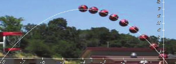
179 H(t) t t t g g h h h g g

180 Section 3.2 Eercises y z p f g ht t t k t f g h k

181 bc bc f bc f bc y y y y y y ht t t ht t t h h

182 A A A A

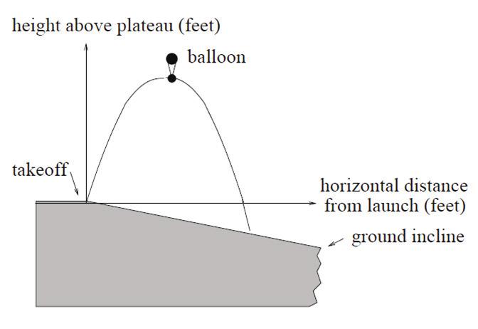
183 f f

184 Section 3.3 Graphs of Polynomial Functions Short run Behavior: Intercepts f f() gt t t g() g

185 g(t) t t t t t t t ht t t t t t hhh f t t t Graphical Behavior at Intercepts f

186 multiplicity p h h p p p f

187 f f Solving Polynomial Inequalities

188 f f() vt t t t t t t t t tt t t t v(t)

189 g Writing Equations using Intercepts n p n n p p a f pi a a f a

190 a a a f Estimating Etrema w w w

191 ww w w w w w w w w V w f

192 g g f

193 Section 3.3 Eercises Ct Ct t t t Ct t t t Ct tt t Ct tt t Ct t t t Ct t t t f g t t ht t t t k t t t t p t ttt qt t tt f g h k m n f g h k n m p t t t qt

194

195 y y

196 Section 3.4 Rational Functions t v vt vt tv v v inversely proportional y f inversely proportional to the square VdV k f k d

197 f f f Short run behavior: f f vertical asymptote Long run behavior: f horizontal asymptote f vertical asymptotea a a f horizontal asymptote y b f b

198 f f f f y f f

199 rational function P()Q() p P a aa a f p q Q bbb b q t water t sugar t C t Ct t Finding Asymptotes and Intercepts k

200 k vertical asymptotes hole

201 Case 1: f f g y f Case 2: f f g f f f f Case 3: f

202 f g f y horizontal asymptote y t Ct t t t t Ct y f

203 f y f Intercepts f f

204 f

205 f f y

206 f n m v v v n n q m q q p n p p v v v a f piqi a

207 a f a a a f f f f f

208 y f f y f y

209 Section 3.4 Eercises A A f g h B B A B k A B p q s r f g a h n w b k m z

210 y y y y y y

211

212 n n n n a b m c d m

213 pnn an b pn cn d C k d C k d k

214 Section 3.5 Inverses and Radical Functions y y y a a a a y y

215 is y y y y y y Area y radical functions f f()y y y y y

216 f y y y a b cy y y y f f y y y y f y

217 v vd gfd g d f fd v f

218 f() f() or n Cn n n n C n C n n C Cn n n C n Cn n C Cn C nc C n f

219 f y y y f y y

220 Section 3.5 Eercises f f f f f f f f f f f f f f f f v L v L v r v r

221 A A y h fh h g h h

222 w f t wt t f w

223 Chapter 4: Eponential and Logarithmic Functions Section 4.1 Eponential Functions Pt number f percent A B A B Precalculus: An Investigation of Functions

224 B n n Bn eponential growth or decay function f a r f ab br a r b b AB

225 B A B A t r f a r t f t t f

226 r m f m f m m m f At t Bt t a r d d Qd Q

227 T(q) T br T Finding Equations of Eponential Functions t a t f t b b b b b t f t br r n

228 ab f r a f br b ab f ab ab ab ab a a b b ab a b b b b b b a a b a f

229 ab ab a b a a ab b b b b b b b b b a b a f

230 Compound Interest compounding nominal rateannual percentage rate (APR) rk r/k tkt Compound Interest kt r A t a k A(t) t a r k a r k A t A

231 r k a aa a a a A more annual percentage yield (APY)

232 k r A a k k r a a k k r a k annual percentage yield k r APY k APY APY A Limit to Compounding

233 Frequency Value e k e k k e e ee ep()ep()e ee continuous growth f e Continuous Growth r f ae a r

234 r f e t St e S(t) ra f e f a r actual t f t e f t t

235 f

236 Section 4.1 Eercises f() h() g() k() m() n()

237

238 t P t e t P t e t t wt t wt t at t at bt

239

240 Section 4.2 Graphs of Eponential Functions f f() g g() f f g

241 f ab a a b f ab a ba b > b y a a aab b b > f f b f f f b a f f

242 ab a b b ab aa b a a

243 f g h k k() h() f()g()g() g() f() h() k() f g h Transformations of Eponential Graphs a

244 f f f f f y y f f ab f ab f ab c y = c a+c f e y

245 f y g g f f

246 y ab f ab a a a ab b b b b b f

247 h g f f e f f f f

248 Section 4.2 Eercises f f f f f f f ab b B A B A C C D D E F E b F a a f f g h f f k f f f f f f f y

249 f f f f f f f

250 Section 4.3 Logarithmic Functions f g log The logarithmb b b b b b b b

251 f a c f c a b a c b c a a c b a b bc bb c b a b c f(c) b c

252 common log natural loge Values of the common log

253 e e e e e e e r b A r b A A b b A r A r b A b r r b A r b A A b b r r b A A b p q b b r b A r b A pq

254 c A b A c b b A b Ac c b c A c b c A c A c A b A c b c b e e e

255

256 t t f t tf(t) t t t t t H ph H

257 H H H rt t Pt ae P P r ae a e r r e r e r r k r k a r ae k r e k r e k r

258 t St e t k r e r e t St

259 Section 4.3 Eercises q m t k a c p v t r s w n y y y d c k z n L a b p v k e h y e e e e e t t t t t e t e

260 kt f t ae f t t f t t f t t f t t t f t ab t t f t e f t e t f t e t f t e

261 Section 4.4 Logarithmic Properties Inverse Properties: b b b b Eponential Property: r b A r b A Change of Base: c A b A c b Sum of Logs Property: A C AC b b b Difference of Logs Property: A b A b C b C not A BAB a A c C b b a A b c C b

262 AC b a b c ac AC b ac b AC b b a c ac b AC b A b C

263 y y y y y y y value log(value)

264 ph H CP P C C ph C ph C C C P C ph P P Log properties in solving equations

265 t t Kenyat t Sudant t t t t t t

266 t t t t t t t t t t t t t t t t t

267 t

268 Section 4.4 Eercises yz y z y ab z c a b c a b c y y y y y y y y y

269 e t t e e t e t

270 Section 4.5 Graphs of Logarithmic Functions f f() g g() f f g b b b

271 f f

272 Transformations of the Logarithmic Function b b c c c c b b c c f c c f c f g e e g f g

273 f f f f f f

274 f ab k f abk = b f a k a k a k k a a a f f

275 f f

276 Section 4.5 Eercises f f f f f f f f f g f f g f f f f f

277

278 Section 4.6 Eponential and Logarithmic Models Radioactive Decay half-life t ht ab t a ab t b a d Qd a a d a a a d d d d

279 d t Qt a r a a r a r r r

280 r ae a a r e r e r r t ae Q t t Q(t)a t ae a t e t e t t

281 Doubling Time doubling time t ht ab a ab b tt t Ct ab t a Ct b b b b t Ct C(t)a t a a t t t t

282 a rt Nt e t r e r e r r t Nt e N e Newton s Law of Cooling

283 TTs s kt T ae t T t a k s t T ab t T kt ae t T T a a ae k T k k e k k e e k k t e t T

284 t e e t e t t t Logarithmic Scales Planet Distance (millions of km)

285 Planet Distance (millions of km) log(distance) P A B C D P PV V V

286 ABCD BAD Clinear relative order of magnitude

287 BAD C ABorders of magnitudea B B A CB B C CB S S S M S

288 S S S S S S S S S S S S S S S

289 S S S S S S S S S S S S S S M M S S S S M S S M S S M S S M multiplying add

290 r

291 Section 4.6 Eercises

292 t t nt e t t nt e

293 t P t t e t N t t e W m W m W m g g g

294 t t t f t e f t t I Id d I d t

295 p Y Mp p pm p Y Hp p p M p Hp p p Mp Hp Mp Hp t L t e L t t L t

296 t Ct t t

297 Section 4.7 Fitting Eponential Models to Data

298 semi-log semi-log log-log f f() log(f())

299 (f()) f ab f() f ab f a b f a b ab g() g() g (g())

300 g() g g g g g g() (g()) Fitting Eponential Functions to Data f()bm f()

301 t Ct t C(t) t Ct Ct Ct t t t Ct

302 t C V, t t V f t Vt V

303 Section 4.7 Eercises f mb f f f f y y y y

304 y

305 Chapter 5: Systems of Equations Section 5.1: Systems in Two Variables n C Cn n Rn Rn n Precalculus

306 Rn Cn n n n n n R C b p

307 bb p p b p b p b p b p b, p bp p p b p b

308 y y y y y y y y y y

309 y y y Solving a System by Substitution y y y y y y y

310 y y y y y y y y

311 a b ab a b ab ab a b a b b bb b b a ba a a Solving a System by the Addition Method

312 y- y y y y y y y y y y

313 y y y y y y y y y y y y

314 y y y y y y y y y y y y y y

315 y y y y y y y - y - y y y y y

316 y y y b p b p p b p b p b b b

317 p p p p bp Dependent and Inconsistent Systems consistent system independent system dependentsystem y- inconsistent system y- independent system y inconsistent system dependent system

318 y y y. y y y y y y y y y y

319 y y y y y - y y y y y y y

320 y y y y y y y y y y y

321 Section 5.1 Eercises y y y y y y y y y y y y y y y y y y y y y y y y y y y y y y y y y y

322 y y y y y y y y y y y y y y y y y y y y y y y y y y y y y y y y y y y y

323 y y y y y y y y y y C R C R C R C C

324 Section 5.2: Systems in Three Variables rtp rrt tpp rtp rtp rtp, y solution set yz

325 yz yz yz y z yz yz yz yz yz yz

326 yz yz yz yz yz yz z yz yz z yz yz z z y y y y z y Gaussian elimination

327 yz AByCz D Ey Fz G Hz K z y yz yz yz yz yz yz yz yz yz yz yz yz yz yz yz

328 yz yz yz yz yz z yz yz z z z zy y y y y yz yz yz yz

329 rtp t p rt p r rtp rt p t p rr rtp rtp t p rtp t p t p rtp tp t p rtp tp p p p p pt

330 t t t t ptr r r r Number of Possible Solutions: Dependent and Inconsistent Systems yz

331 yz yz yz yz yz yz yz yz yz yz yz

332 y z yz y z yz yz yz y z z z z z z y y y y y

333 y z y yz y z yz y z yz y z

334 Section 5.2 Eercises y z y z y z y z y z y y z y y z z y z y z y z y z y z y z y z y z y z y z y z y z y z y z y z y z y z y z y z y z y z y z y z y z y z y z y y z z y z y z y z y z y z y z

335 y z y z y z y z y z y z y z y z y z y z y z y z y z y z y z y z z y z y z y z y z z z y yz y z y z y z yz y z y z y z y z y z y z y z y z y z y z y z y z y z

336 y z y z y z y z y z y z y z y z y z y z y z y z y z y z y z y z y z y z y z y z y z y z y z y z y z y z y z y z y z y z y z y z y z

337 Section 5.3: Linear Inequalities equation f y yinequality y y y y y y y y y

338 y y y y y y y y y y

339 p c pc pc pc p c c c c p p

340 Systems of Linear Inequalities y y

341 bp b p b p b p

342

343 Section 5.4: Solving Systems using Matrices Writing the Augmented Matri of a System of Equations augmented matri - y- z y y coefficient matri

344 yz y z y z - a byczd y y Writing a System of Equations from an Augmented Matri

345 y z yz yz yz Performing Row Operations on a Matri row operations rowechelon formmain diagonal a b d row-equivalent leading

346 Ri Rj cri R cr i j Gaussian Elimination Gaussian elimination A a a a b b A a a a A b a a a

347 y y R R RR R R R y y

348 y y y y R R R R R y y A

349 R R R R R y y y y y RR R R R R

350 R R R R R yz y yz Solving a 3-by-3 System of Linear Equations Using Matrices y z y z y z

351 RR R RR R R R R R R R R R R yz yz z yz y yz

352 R R R RR R R R R yz yz y z yz y z z z z z

353 z y yz z y y yz yz yz y z

354 yz yz yz yz RR R RR R R R R R R R z y z yz z

355 y y y y yz y z y z y z y z

356 Section 5.4 Eercises y y y y y z y z y z y z y z y z y z y

357 y y y y y y y y y y y y y y y y y y y y y y y y

358 y z y z y z y z y z y z y z y z y z y z y z y z y z y z y z y z y z z y z y z z y z y y z y z y z

359 Section 5.5: Matrices and Matri Operations Wildcats Mud Cats Goals Balls Jerseys Finding the Sum and Difference of Two Matrices matri row column. entry A B C A B C Describing Matrices mn m n A aij i j A a a a a A a a a a a a nn

360 n a a a m a a a matri A B C entry a i row j column mn m n A A a a a a Adding and Subtracting Matrices ij

361 addition and subtraction of matrices is only possible when the matrices have the same dimensions A B A B C D ABCa ij b ij c ij ABDa ij b ij d ij ABBA AB C A BC A B a b e f A B c d g h a b e f A B c d g h ae b f cg d h A B A B

362 A B A B A B A B Finding Scalar Multiples of a Matri scalar multiple

363 Lab A Lab B Computers Computer Tables Chairs C C C C

364 a a A a a ca ca c a a a a ca ca ca ca A B C a b aabaaab abaaaba A A A A B B B

365 A B A B A B A B A B AB Finding the Product of Two Matrices

366 A mr B rn AB mn AB A B A B A B i AB i A j B A B A B AB b b b a a a A B b b b a a a b b b AB A B b a a a b a b a b a b b AB A B b a a a b a b a b a b b AB A B b a a a b a b a b a b b

367 AB A B A B A B a b a b a b a b a b a b a b a b a b AB a b a b a b a b a b a b a b a b a b A B C ABC ABC CABCACB ABC ACBC A B A B A B AB A B AB BA

368 A B A B A B A B AB B A BA AB BA AB BA

369 Wildcats Mud Cats Goals Balls Jerseys Goal Ball Jersey E C CE

370 A B B

371 Section 5.5 Eercises AB BA AB BA A B C D E F A B C D A C B E C F D B A B C D A B B C C D

372 A B C D AB BC CA BD DC CB A B C D E A B C AD C B D E CD D E A AA A B C AB BA CA BC A B C B A A B AB BA

373 A AA A B C D AB BA BD DC D A D ABC ABC

374

375 Chapter 6: Sequences and Series Section 6.1: Sequences Writing the Terms of a Sequence Defined by an Eplicit Formula sequence term eplicitformula nth term of the sequence n n Precalculus

376 n n abc n a n n n n a n n n n an n n infinite sequence n finite sequence

377 n a aa a a n a a a a n n n a a a n n a a n n n a n n n n n a n a n a n a n a

378 n an t n n Investigating Alternating Sequences n

379 n n n a n a n n n n an n n n n a n a n a n a n a n n n n

380 n an n Finding an Eplicit Formula n an n n n n n e e e e e n n n

381 n n an n n n an n e n e n n an e n n e e ee Writing the Terms of a Sequence Defined by a Recursive Formula recursive formula

382 an a an an n a a a a a a a a a an an ann a a a recursive formula

383 n a a a n a n a an an n an n a n a a n a a n a a n a a a a a n n n n a a n

384 a a an an ann aa n a a a n a aa n a a a n a a a a a a an an ann a n Using Factorial Notation n factorial n n

385 a n n n a n nn n factorial n n, n nn n n n n an n n n n a n a n a n a n a

386 n a n n a n a n n n an e n n n n

387 Section 6.1 Eercises a n n

388

389

390 Section 6.2: Arithmetic Sequences Finding Common Differences arithmetic sequence common difference arithmetic sequence common difference a d an a ad ad ad

391 a b

392 Writing Terms of Arithmetic Sequences n d a a n d n a d a d a a a n d a n n d a n d an a n d n

393 a a a d d d d a d d d an a nd a d a ad a d a a an a nd a a a Using Recursive Formulas for Arithmetic Sequences a a d n n n d a a d n n n

394 d a an an n Using Eplicit Formulas for Arithmetic Sequences an a dn

395 y y y y m b an yn mb an n an n a n n n an a dn a a a a dn n

396 d a a an n an n Finding the Number of Terms in a Finite Arithmetic Sequence d a n a dn an n

397 n an a dn an n an n an n n n Solving Application Problems with Arithmetic Sequences a a an a dn

398 A n An n A n a a an an n an n Tn n

399 Section 6.2 Eercises

400

401

402 Section 6.3: Geometric Sequences Finding Common Ratios geometric sequence common ratio geometric sequence common ratio a r aar ar ar

403

404 Writing Terms of Geometric Sequences a r a a a a a a a a a a a r a a a a a a a a a a a a r

405 Using Recursive Formulas for Geometric Sequences r a a n ran n r a an ran an an n a

406 Using Eplicit Formulas for Geometric Sequences n an ar a n n n n an ar a a a r rr r n an ar a r a r a r r r

407 a a a a a n n an ar n an

408 Solving Application Problems with Geometric Sequences a a n an ar P n P n n n P

409 a an an n a n a n P n n

410 Section 6.3 Eercises

411

412

413 Section 6.4: Series Using Summation Notation series nthpartial sum S n S S S S Summation notation inde of summation lower limit of summation upper limit of summation ak k k k k a a a a a

414 k k n series summation notation n k a k ak k k nkinde of summationlower limit of summationnupper limit of summation k k k k k k k k k k

415 k k Using the Formula for Arithmetic Series d arithmetic series n S n a a d a d a n d a n S n a n a n d a n d a d a n n Sn aad ad an d an S a a d a d a d a n n n n S a a a a a a n n n n n S n na a n n na an Sn n arithmetic series n na an Sn n a an n na a a an n Sn S n n

416 k k a a n n a an n na an Sn S a a n n an a nd n n n n a an n n a an Sn S a k k ak a n a k ak k a a an n S n n a a n

417 S k k a d n S a an a dn a na an Sn S

418 Using the Formula for Geometric Series geometric series r n S n a ra r a r n a n r n rsn rar ar ar a n Sn arar ar a n rsn rar ar ar a n rs n ara S n r n a r Sn r r n geometric series n n a r Sn r r n a r n a r n S n a r n r S n S k k

419 a n r r a r n n a r Sn r S a k a r n a r n S S n a r r n S k k

420 a n r a r n n a r Sn r S Using the Formula for the Sum of Infinite Geometric Series n infinite series k k diverges Determining Whether the Sum of an Infinite Geometric Series is Defined rn r n r r

421 r r r k k k k

422 k k Finding Sums of Infinite Series n n a r Sn r r rn n n r n n n n r n r n n r r a a S r r a S r

423 a r r a r S a r S k k k k a r a r S a r S r a k a a r S a r S r

424 a S n r k k k k Solving Annuity Problems annuity a r

425 n n n a r n S a n r r a r n n S n a r n r S n n a n r r a r n n

426 S r

427 Section 6.4 Eercises n n n n n a a n

428 m m k k k k Sn a n a n k k k n n k

429 k k n k k n n k n k n

430

431 Solutions to Selected Eercises Chapter 1 Section 1.1 f f f g g f f f f f f f y height height of head postage age time weight t a r

432 Section 1.2 t g t f f f f if if f if f if if if f if if

433 Section 1.3 b h h h h

434 Section 1.4 f g g f f g g f f g f g f g g f g f g f f g h rv t t f g g f f g f g f f a ab b a abb g g C f s s s C gh h h vcm m m

435 Section 1.5 f f g f h f y y y f f y y

436 f() y f()yy f f f

437 a f f f f f f y y y

438 y y y Domain Range y Section 1.6 f f f f f f gf f g Chapter 2 Section 2.1 P t t D t t Mn n

439 y y y y y y Pnn g f k C F F C F Section 2.2

440 g y m m m m m m y y t Section 2.3 P t t C P t t R t t b A m

441 Section 2.4 y r y r situps r Section 2.5 y y or or or