Development of Beam Equations

Transcription

1 CHAPTER 4 Development of Beam Equations Introduction We begin this chapter by developing the stiffness matrix for the bending of a beam element, the most common of all structural elements as evidenced by its prominence in buildings, bridges, towers, and many other structures. The beam element is considered to be straight and to have constant cross-sectional area. We will first derive the beam element stiffness matrix by using the principles developed for simple beam theory. We will then present simple examples to illustrate the assemblage of beam element stiffness matrices and the solution of beam problems by the direct stiffness method presented in Chapter. The solution of a beam problem illustrates that the degrees of freedom associated with a node are a transverse displacement and a rotation. We will include the nodal shear forces and bending moments and the resulting shear force and bending moment diagrams as part of the total solution. Next, we will discuss procedures for handling distributed loading, because beams and frames are often subjected to distributed loading as well as concentrated nodal loading. We will follow the discussion with solutions of beams subjected to distributed loading and compare a finite element solution to an exact solution for a beam subjected to a distributed loading. We will then develop the beam element stiffness matrix for a beam element with a nodal hinge and illustrate the solution of a beam with an internal hinge. To further acquaint you with the potential energy approach for developing stiffness matrices and equations, we will again develop the beam bending element equations using this approach. We hope to increase your confidence in this approach. It will be used throughout much of this text to develop stiffness matrices and equations for more complex elements, such as two-dimensional (plane) stress, axisymmetric, and three-dimensional stress. Finally, the Galerkin residual method is applied to derive the beam element equations. 151

2 15 d 4 Development of Beam Equations The concepts presented in this chapter are prerequisite to understanding the concepts for frame analysis presented in Chapter 5. d 4.1 Beam Stiffness In this section, we will derive the stiffness matrix for a simple beam element. A beam is a long, slender structural member generally subjected to transverse loading that produces significant bending effects as opposed to twisting or axial effects. This bending deformation is measured as a transverse displacement and a rotation. Hence, the degrees of freedom considered per node are a transverse displacement and a rotation (as opposed to only an axial displacement for the bar element of Chapter ). Consider the beam element shown in Figure 4 1. The beam is of length L with axial local coordinate ^x and transverse local coordinate ^y. The local transverse nodal displacements are given by ^d iy s and the rotations by ^f i s. The local nodal forces are given by ^f iy s and the bending moments by ^m i s as shown. We initially neglect all axial effects. At all nodes, the following sign conventions are used: 1. Moments are positive in the counterclockwise direction.. Rotations are positive in the counterclockwise direction.. Forces are positive in the positive ^y direction. 4. Displacements are positive in the positive ^y direction. Figure 4 indicates the sign conventions used in simple beam theory for positive shear forces ^V and bending moments ^m. d Figure 4 1 moments Beam element with positive nodal displacements, rotations, forces, and Figure 4 Beam theory sign conventions for shear forces and bending moments

3 4.1 Beam Stiffness d 15 y, ˆ ˆ w(x) ˆ fˆ xˆ a c b d a b c d (a) Undeformed beam under load w(x) ˆ (b) Deformed beam due to applied loading (c) Differential beam element Figure 4 Beam under distributed load Beam Stiffness Matrix Based on Euler-Bernouli Beam Theory (Considering Bending Deformations Only) The differential equation governing elementary linear-elastic beam behavior [1] (called the Euler-Bernoulli beam as derived by Euler and Bernoulli) is based on plane cross sections perpendicular to the longitudinal centroidal axis of the beam before bending occurs remaining plane and perpendicular to the longitudinal axis after bending occurs. This is illustrated in Figure 4, where a plane through vertical line a c (Figure 4 (a)) is perpendicular to the longitudinal ^x axis before bending, and this same plane through a c (rotating through angle ^f in Figure 4 (b)) remains perpendicular to the bent ^x axis after bending. This occurs in practice only when a pure couple or constant moment exists in the beam. However it is a reasonable assumption that yields equations that quite accurately predict beam behavior for most practical beams. The differential equation is derived as follows. Consider the beam shown in Figure 4 subjected to a distributed loading wð^xþ (force/length). From force and moment equilibrium of a differential element of the beam, shown in Figure 4 (c), we have SF y ¼ : V ðv þ dvþ wð^xþ dx ¼ (4.1.1a) Or, simplifying Eq. (4.1.1a), we obtain wd^x dv ¼ or w ¼ dv (4.1.1b) d ^x SM ¼ : V dxþ dm þ wð^xþ d ^x d ^x ¼ or V ¼ dm (4.1.1c) d ^x The final form of Eq. (4.1.1c), relating the shear force to the bending moment, is obtained by dividing the left equation by d ^x and then taking the limit of the equation as d ^x approaches. The wð^xþ term then disappears.

4 154 d 4 Development of Beam Equations Figure 4 4 Deflected curve of beam Also, the curvature k of the beam is related to the moment by k ¼ 1 r ¼ M EI (4.1.1d) where r is the radius of the deflected curve shown in Figure 4 4b, ^v is the transverse displacement function in the ^y direction (see Figure 4 4a), E is the modulus of elasticity, and I is the principal moment of inertia about the ^z axis (where the ^z axis is perpendicular to the ^x and ^y axes). The curvature for small slopes ^f ¼ d^v=d ^x is given by k ¼ d ^v (4.1.1e) d ^x Using Eq. (4.1.1e) in (4.1.1d), we obtain d ^v d ^x ¼ M (4.1.1f ) EI Solving Eq. (4.1.1f ) for M and substituting this result into (4.1.1c) and (4.1.1b), we obtain d EI d ^v ¼ wð^xþ d ^x d ^x (4.1.1g) For constant EI and only nodal forces and moments, Eq. (4.1.1g) becomes EI d 4^v d ^x ¼ (4.1.1h) 4 We will now follow the steps outlined in Chapter 1 to develop the stiffness matrix and equations for a beam element and then to illustrate complete solutions for beams. Step 1 Select the Element Type Represent the beam by labeling nodes at each end and in general by labeling the element number (Figure 4 1).

5 4.1 Beam Stiffness d 155 Step Select a Displacement Function Assume the transverse displacement variation through the element length to be ^vð^xþ ¼a 1 ^x þ a ^x þ a ^x þ a 4 ð4:1:þ The complete cubic displacement function Eq. (4.1.) is appropriate because there are four total degrees of freedom (a transverse displacement ^d iy and a small rotation ^f i at each node). The cubic function also satisfies the basic beam differential equation further justifying its selection. In addition, the cubic function also satisfies the conditions of displacement and slope continuity at nodes shared by two elements. Using the same procedure as described in Section., we express ^v as a function of the nodal degrees of freedom ^d 1y, ^d y, ^f 1, and ^f as follows: ^vðþ ¼^d 1y ¼ a 4 d^vðþ d ^x ¼ ^f 1 ¼ a ð4:1:þ ^vðlþ ¼^d y ¼ a 1 L þ a L þ a L þ a 4 d^vðlþ d ^x ¼ ^f ¼ a 1 L þ a L þ a where ^f ¼ d^v=d ^x for the assumed small rotation ^f. Solving Eqs. (4.1.) for a 1 through a 4 in terms of the nodal degrees of freedom and substituting into Eq. (4.1.), we have ^v ¼ L ð^d 1y ^d y Þþ 1 L ð ^f 1 þ ^f Þ ^x þ L ð^d 1y ^d y Þ 1 L ð ^f 1 þ ^f Þ ^x þ ^f 1 ^x þ ^d 1y ð4:1:4þ In matrix form, we express Eq. (4.1.4) as ^v ¼½NŠf^dg ^d 1y ^f f^dg ¼ 1 where ^d y ^f ð4:1:5þ (4.1.a) and where ½NŠ ¼½N 1 N N N 4 Š (4.1.b) and N 1 ¼ 1 L ð^x ^x L þ L Þ N ¼ 1 L ð^x L ^x L þ ^xl Þ ð4:1:7þ N ¼ 1 L ð ^x þ ^x LÞ N 4 ¼ 1 L ð^x L ^x L Þ N 1, N, N,andN 4 are called the shape functions for a beam element. These cubic shape (or interpolation) functions are known as Hermite cubic interpolation (or cubic

6 15 d 4 Development of Beam Equations spline) functions. For the beam element, N 1 ¼ 1 when evaluated at node 1 and N 1 ¼ when evaluated at node. Because N is associated with ^f 1, we have, from the second of Eqs. (4.1.7), ðdn =d ^xþ ¼1 when evaluated at node 1. Shape functions N and N 4 have analogous results for node. Step Define the Strain=Displacement and Stress=Strain Relationships Assume the following axial strain/displacement relationship to be valid: e x ð^x; ^yþ ¼ d ^u ð4:1:þ d ^x where ^u is the axial displacement function. From the deformed configuration of the beam shown in Figure 4 5, we relate the axial displacement to the transverse displacement by ^u ¼ ^y d^v ð4:1:þ d ^x where we should recall from elementary beam theory [1] the basic assumption that cross sections of the beam (such as cross section ABCD) that are planar before bending deformation remain planar after deformation and, in general, rotate through a small angle ðd^v=d ^xþ. Using Eq. (4.1.) in Eq. (4.1.), we obtain e x ð^x; ^yþ ¼ ^y d ^v d ^x ð4:1:1þ yˆ d ˆ ˆ dxˆ = f (c) Figure 4 5 Beam segment (a) before deformation and (b) after deformation; (c) angle of rotation of cross section ABCD

7 4.1 Beam Stiffness d 157 From elementary beam theory, the bending moment and shear force are related to the transverse displacement function. Because we will use these relationships in the derivation of the beam element stiffness matrix, we now present them as Step 4 ^mð^xþ ¼EI d ^v d ^x ^V ¼ EI d ^v d ^x Derive the Element Stiffness Matrix and Equations ð4:1:11þ First, derive the element stiffness matrix and equations using a direct equilibrium approach. We now relate the nodal and beam theory sign conventions for shear forces and bending moments (Figures 4 1 and 4 ), along with Eqs. (4.1.4) and (4.1.11), to obtain ^f 1y ¼ ^V ¼ EI d ^vðþ d ^x ^m 1 ¼ ^m ¼ EI d ^vðþ d ^x ^f y ¼ ^V ¼ EI d ^vðlþ d ^x ^m ¼ ^m ¼ EI d ^vðlþ d ^x ¼ EI L ð1^d 1y þ L ^f 1 1^d y þ L ^f Þ ¼ EI L ðl^d 1y þ 4L ^f1 L^d y þ L ^f Þ ¼ EI L ð 1^d 1y L ^f 1 þ 1^d y L ^f Þ ¼ EI L ðl^d 1y þ L ^f1 L^d y þ 4L ^f Þ ð4:1:1þ where the minus signs in the second and third of Eqs. (4.1.1) are the result of opposite nodal and beam theory positive bending moment conventions at node 1 and opposite nodal and beam theory positive shear force conventions at node as seen by comparing Figures 4 1 and 4. Equations (4.1.1) relate the nodal forces to the nodal displacements. In matrix form, Eqs. (4.1.1) become 1 L 1 L ^d 1y ^f 1y ^m 1 ^f y ^m ¼ EI L 4 L 4L L L 1 L 1 L L L L 4L where the stiffness matrix is then 1 L 1 L ^k ¼ EI L 4L L L 7 L 4 1 L 1 L 5 L L L 4L ^f ^d y ^f ð4:1:1þ ð4:1:14þ Equation (4.1.1) indicates that ^k relates transverse forces and bending moments to transverse displacements and rotations, whereas axial effects have been neglected. In the beam element stiffness matrix (Eq. (4.1.14) derived in this section, it is assumed that the beam is long and slender; that is, the length, L, to depth, h, dimension ratio of the beam is large. In this case, the deflection due to bending that is predicted by using the stiffness matrix from Eq. (4.1.14) is quite adequate. However, for short, deep beams the transverse shear deformation can be significant and can

8 15 d 4 Development of Beam Equations have the same order of magnitude contribution to the total deformation of the beam. This is seen by the expressions for the bending and shear contributions to the deflection of a beam, where the bending contribution is of order ðl=hþ, whereas the shear contribution is only of order ðl=hþ. A general rule for rectangular cross-section beams, is that for a length at least eight times the depth, the transverse shear deflection is less than five percent of the bending deflection [4]. Castigliano s method for finding beam and frame deflections is a convenient way to include the effects of the transverse shear term as shown in [4]. The derivation of the stiffness matrix for a beam including the transverse shear deformation contribution is given in a number of references [5 ]. The inclusion of the shear deformation in beam theory with application to vibration problems was developed by Timoshenko and is known as the Timoshenko beam [ 1]. Beam Stiffness Matrix Based on Timoshenko Beam Theory (Including Transverse Shear Deformation) The shear deformation beam theory is derived as follows. Instead of plane sections remaining plane after bending occurs as shown previously in Figure 4 5, the shear deformation (deformation due to the shear force V ) is now included. Referring to Figure 4, we observe a section of a beam of differential length d ^x with the cross section assumed to remain plane but no longer perpendicular to the neutral axis V dxˆ ˆ (x) ˆ V + xˆ b(x) ˆ f(x) ˆ ˆ M M + xˆ xˆ (a) fˆ (1) (1) d ˆ dxˆ Element 1 fˆ () (b) () d ˆ dxˆ Element fˆ (1) = f ˆ () (1) () d ˆ d ˆ dxˆ dxˆ Figure 4 (a) Element of Timoshenko beam showing shear deformation. Cross sections are no longer perpendicular to the neutral axis line. (b) Two beam elements meeting at node

9 4.1 Beam Stiffness d 15 (^x axis) due to the inclusion of the shear force resulting in a rotation term indicated by b. The total deflection of the beam at a point ^x now consists of two parts, one caused by bending and one by shear force, so that the slope of the deflected curve at point ^x is now given by d^v d ^x ¼ ^fð^xþþbð^xþ ð4:1:15aþ where rotation due to bending moment and due to transverse shear force are given, respectively, by ^f ð^xþ and bð^xþ. We assume as usual that the linear deflection and angular deflection (slope) are small. The relation between bending moment and bending deformation (curvature) is now d Mð^xÞ ¼EI ^f ð^xþ ð4:1:15bþ d ^x and the relation between the shear force and shear deformation (rotation due to shear) (shear strain) is given by Vð^xÞ ¼k s AGbð^xÞ ð4:1:15cþ The difference in d^v=d ^x and ^f represents the shear strain g yz ð¼ bþ of the beam as g yz ¼ d^v ^f ð4:1:15dþ d ^x Now consider the differential element in Figure 4 c and Eqs. (4.1.1b) and (4.1.1c) obtained from summing transverse forces and then summing bending moments. We now substitute Eq. (4.1.15c) for V and Eq. (4.1.15b) for M into Eqs. (4.1.1b) and (4.1.1c) along with b from Eq. (4.1.15a) to obtain the two governing differential equations as d d ^x d d ^x k sag d^v ^f d ^x ¼ w! d ^f EI þ k s AG d^v ^f ¼ d ^x d ^x ð4:1:15eþ ð4:1:15fþ To derive the stiffness matrix for the beam element including transverse shear deformation, we assume the transverse displacement to be given by the cubic function in Eq. (4.1.). In a manner similar to [], we choose transverse shear strain g consistent with the cubic polynomial for ^vð^xþ, such that g is a constant given by g ¼ c ð4:1:15gþ Using the cubic displacement function for ^v, the slope relation given by Eq. (4.1.15a), and the shear strain Eq. (4.1.15g), along with the bending moment-curvature relation, Eq. (4.1.15b) and the shear force-shear strain relation Eq. (4.1.15c), in the bending moment shear force relation Eq. (4.1.1c), we obtain c ¼ a 1 g ð4:1:15hþ where g ¼ EI=k s AG and k s A is the shear area. Shear areas, A s vary with crosssection shapes. For instance, for a rectangular shape A s is taken as 5/ times the

10 1 d 4 Development of Beam Equations cross section A, for a solid circular cross section it is taken as. times the cross section, for a wide-flange cross section it is taken as the thickness of the web times the full depth of the wide-flange, and for thin-walled cross sections it is taken as two times the product of the thickness of the wall times the depth of the cross section. Using Eqs. (4.1.), (4.1.15a), (4.1.15g), and (4.1.15h) allow f to be expressed as a polynomial in ^x as follows: ^f ¼ a þ a ^x þð^x þ gþa 1 ð4:1:15iþ Using Eqs. (4.1.) and (4.1.15i), we can now express the coefficients a 1 through a 4 in terms of the nodal displacements ^d 1y and ^d y and rotations ^f 1 and ^f of the beam at the ends ^x ¼ and^x ¼ L as previously done to obtain Eq. (4.1.4) when shear deformation was neglected. The expressions for a 1 through a 4 are then given as follows: a 1 ¼ ^d 1y þ L ^f 1 ^d y þ L ^f LðL þ 1gÞ a ¼ L ^d 1y ðl þ gþ ^f 1 þ L ^d y þð L þ gþ ^f LðL þ 1gÞ a ¼ 1g ^d 1y þðl þ glþ ^f 1 þ 1g ^d y gl ^f LðL þ 1gÞ ð4:1:15jþ a 4 ¼ ^d 1y Substituting these a s into Eq. (4.1.), we obtain ^v ¼ ^d 1y þ L ^f 1 ^d y þ L ^f ^x LðL þ 1gÞ L ^d 1y ðl þ gþ ^f 1 þ L ^d y þð L þ gþ ^f LðL þ 1gÞ ^x 1g ^d 1y þðl þ glþ ^f 1 þ 1g ^d y gl ^f LðL þ 1gÞ ^x þ ^d 1y ð4:1:15kþ In a manner similar to step 4 used to derive the stiffness matrix for the beam element without shear deformation included, we have ^f 1y ¼ ^VðÞ ¼EIa 1 ¼ EIð1 ^d 1y þ L ^f 1 1 ^d y þ L ^f Þ LðL þ 1gÞ ^m 1 ¼ ^mðþ ¼ EIa ¼ EI½L ^d 1y þð4l þ 1gÞ ^f 1 L ^d y þðl 1gÞ ^f Š LðL þ 1gÞ ^f y ¼ ^VðLÞ ¼ EIð 1 ^d 1y L ^f 1 þ 1 ^d y L ^f ð4:1:15 lþ Þ LðL þ 1gÞ ^m ¼ ^mðlþ ¼ EI½L ^d 1y þðl 1gÞ ^f 1 L ^d y þð4l þ 1gÞ ^f Š LðL þ 1gÞ where again the minus signs in the second and third of Eqs. ð4:1:15 lþ are the result of opposite nodal and beam theory positive moment conventions at node l and opposite

11 4. Example of Assemblage of Beam Stiffness Matrices d 11 nodal and beam theory positive shear force conventions at node, as seen by comparing Figures 4 and 4 7. In matrix form Eqs ð4:1:15 lþ become ^f 1y 1 L 1 L ^d 1y ^m 1 EI L ð4l þ 1gÞ L ðl 1gÞ ^f ¼ 7 1 ^f y LðL þ 1gÞ 4 1 L 1 L 5 ^d y ^m L ðl 1gÞ L ð4l þ 1gÞ ^f ð4:1:15mþ where the stiffness matrix including both bending and shear deformation is then given by 1 L 1 L EI L ð4l ^k þ 1gÞ L ðl 1gÞ ¼ 7 ð4:1:15nþ LðL þ 1gÞ 4 1 L 1 L 5 L ðl 1gÞ L ð4l þ 1gÞ In Eq. (4.1.15n) remember that g represents the transverse shear term, and if we set g ¼, we obtain Eq. (4.1.14) for the beam stiffness matrix, neglecting transverse shear deformation. To more easily see the effect of the shear correction factor, we define the nondimensional shear correction term as j ¼ 1EI=ðk s AGL Þ¼1g=L and rewrite the stiffness matrix as 1 L 1 L EI L ð4 þ jþl ^k L ð jþl ¼ 7 ð4:1:15oþ L ð1 þ jþ 4 1 L 1 L 5 L ð jþl L ð4 þ jþl Most commercial computer programs, such as [11], will include the shear deformation by having you input the shear area, A s ¼ k s A. d 4. Example of Assemblage of Beam Stiffness Matrices d Step 5 Assemble the Element Equations to Obtain the Global Equations and Introduce Boundary Conditions Consider the beam in Figure 4 7 as an example to illustrate the procedure for assemblage of beam element stiffness matrices. Assume EI to be constant throughout the beam. A force of 1 lb and a moment of 1 lb-ft are applied to the beam at midlength. The left end is a fixed support and the right end is a pin support. First, we discretize the beam into two elements with nodes 1 as shown. We include a node at midlength because applied force and moment exist at midlength and, at this time, loads are assumed to be applied only at nodes. (Another procedure for handling loads applied on elements will be discussed in Section 4.4.)

12 1 d 4 Development of Beam Equations Figure 4 7 Fixed hinged beam subjected to a force and a moment Using Eq. (4.1.14), we find that the global stiffness matrices for the two elements are now given by d 1y f 1 d y f 1 L 1 L k ð1þ ¼ EI L 4L L L ð4::1þ L L 1 L 5 L L L 4L and k ðþ ¼ EI L d y f d y f 1 L 1 L L 4L L L L 1 L 5 L L L 4L ð4::þ where the degrees of freedom associated with each beam element are indicated by the usual labels above the columns in each element stiffness matrix. Here the local coordinate axes for each element coincide with the global x and y axes of the whole beam. Consequently, the local and global stiffness matrices are identical, so hats ð^þ are not needed in Eqs. (4..1) and (4..). The total stiffness matrix can now be assembled for the beam by using the direct stiffness method. When the total (global) stiffness matrix has been assembled, the external global nodal forces are related to the global nodal displacements. Through direct superposition and Eqs. (4..1) and (4..), the governing equations for the beam are thus given by F 1y M 1 F y M F y M ¼ EI L 4 1 L 1 L L 4L L L 1 L 1 þ 1 L þ L 1 L L L L þ L 4L þ 4L L L 1 L 1 L L L L 4L 7 5 d 1y f 1 d y f d y f ð4::þ Now considering the boundary conditions, or constraints, of the fixed support at node 1 and the hinge (pinned) support at node, we have f 1 ¼ d 1y ¼ d y ¼ ð4::4þ

13 4. Examples of Beam Analysis Using the Direct Stiffness Method d 1 On considering the third, fourth, and sixth equations of Eqs. (4..) corresponding to the rows with unknown degrees of freedom and using Eqs. (4..4), we obtain 1 1 ¼ EI 4 L d y 4 L L 7 5 f L ð4::5þ L L 4L f where F y ¼ 1 lb, M ¼ 1 lb-ft, and M ¼ have been substituted into the reduced set of equations. We could now solve Eq. (4..5) simultaneously for the unknown nodal displacement d y and the unknown nodal rotations f and f.we leave the final solution for you to obtain. Section 4. provides complete solutions to beam problems. d 4. Examples of Beam Analysis Using the Direct Stiffness Method Example 4.1 We will now perform complete solutions for beams with various boundary supports and loads to illustrate further the use of the equations developed in Section 4.1. Using the direct stiffness method, solve the problem of the propped cantilever beam subjected to end load P in Figure 4. The beam is assumed to have constant EI and length L. It is supported by a roller at midlength and is built in at the right end. d Figure 4 Propped cantilever beam We have discretized the beam and established global coordinate axes as shown in Figure 4. We will determine the nodal displacements and rotations, the reactions, and the complete shear force and bending moment diagrams. Using Eq. (4.1.14) for each element, along with superposition, we obtain the structure total stiffness matrix by the same method as described in Section 4. for obtaining the stiffness matrix in Eq. (4..). The K is K ¼ EI L d 1y f 1 d y f d y f 1 L 1 L 4L L L 1 þ 1 L þ L 1 L 4L þ 4L L L L 5 Symmetry 4L ð4::1þ

14 14 d 4 Development of Beam Equations The governing equations for the beam are then given by F 1y 1 L 1 L M 1 L 4L L L F y ¼ EI 1 L 4 1 L M L L L L L L 7 F y 4 1 L 1 L 5 L L L 4L M d 1y f 1 d y f d y f ð4::þ On applying the boundary conditions d y ¼ d y ¼ f ¼ ð4::þ and partitioning the equations associated with unknown displacements [the first, second, and fourth equations of Eqs. (4..)] from those equations associated with known displacements in the usual manner, we obtain the final set of equations for a longhand solution as P ¼ EI L 1 L L 4 L 4L L 7 5 L L L d 1y f 1 f ð4::4þ where F 1y ¼ P, M 1 ¼, and M ¼ have been used in Eq. (4..4). We will now solve Eq. (4..4) for the nodal displacement and nodal slopes. We obtain the transverse displacement at node 1 as d 1y ¼ 7PL ð4::5þ 1EI where the minus sign indicates that the displacement of node 1 is downward. The slopes are f 1 ¼ PL f 4EI ¼ PL ð4::þ 4EI where the positive signs indicate counterclockwise rotations at nodes 1 and. We will now determine the global nodal forces. To do this, we substitute the known global nodal displacements and rotations, Eqs. (4..5) and (4..), into Eq. (4..). The resulting equations are F 1y M 1 F y M F y M ¼ EI L 4 1 L 1 L L 4L L L 1 L 4 1 L L L L L L 1 L 1 L L L L 4L 7 5 7PL 1EI PL 4EI PL 4EI ð4::7þ

15 4. Examples of Beam Analysis Using the Direct Stiffness Method d 15 Multiplying the matrices on the right-hand side of Eq. (4..7), we obtain the global nodal forces and moments as F 1y ¼ P M 1 ¼ F y ¼ 5 P ð4::þ M ¼ F y ¼ P M ¼ 1 PL The results of Eqs. (4..) can be interpreted as follows: The value of F 1y ¼ P is the applied force at node 1, as it must be. The values of F y ; F y, and M are the reactions from the supports as felt by the beam. The moments M 1 and M are zero because no applied or reactive moments are present on the beam at node 1 or node. It is generally necessary to determine the local nodal forces associated with each element of a large structure to perform a stress analysis of the entire structure. We will thus consider the forces in element 1 of this example to illustrate this concept (element can be treated similarly). Using Eqs. (4..5) and (4..) in the ^f ¼ ^k ^d equation for element 1 [also see Eq. (4.1.1)], we have ^f 1y ^m 1 ^f y ^m ¼ EI L 4 1 L 1 L L 4L L L 1 L 1 L L L L 4L 7 5 7PL 1EI PL 4EI PL 4EI ð4::þ where, again, because the local coordinate axes of the element coincide with the global axes of the whole beam, we have used the relationships d ¼ ^d and k ¼ ^k (that is, the local nodal displacements are also the global nodal displacements, and so forth). Equation (4..) yields ^f 1y ¼ P ^m 1 ¼ ^fy ¼ P ^m ¼ PL ð4::1þ A free-body diagram of element 1, shown in Figure 4 (a), should help you to understand the results of Eqs. (4..1). The figure shows a nodal transverse force of negative P at node 1 and of positive P and negative moment PL at node. These values are consistent with the results given by Eqs. (4..1). For completeness, the free-body diagram of element is shown in Figure 4 (b). We can easily verify the element nodal forces by writing an equation similar to Eq. (4..). Figure 4 Free-body diagrams showing forces and moments on (a) element 1 and (b) element

16 1 d 4 Development of Beam Equations Figure 4 1 Nodal forces and moment on the beam Figure 4 11 Shear force diagram for the beam of Figure 4 1 Figure 4 1 Bending moment diagram for the beam of Figure 4 1 From the results of Eqs. (4..), the nodal forces and moments for the whole beam are shown on the beam in Figure 4 1. Using the beam sign conventions established in Section 4.1, we obtain the shear force V and bending moment M diagrams shown in Figures 4 11 and 4 1. Example 4. In general, for complex beam structures, we will use the element local forces to determine the shear force and bending moment diagrams for each element. We can then use these values for design purposes. Chapter 5 will further discuss this concept as used in computer codes. Determine the nodal displacements and rotations, global nodal forces, and element forces for the beam shown in Figure 4 1. We have discretized the beam as indicated by the node numbering. The beam is fixed at nodes 1 and 5 and has a roller support at node. Vertical loads of 1, lb each are applied at nodes and 4. Let E ¼ 1 psi and I ¼ 5 in 4 throughout the beam. We must have consistent units; therefore, the 1-ft lengths in Figure 4 1 will be converted to 1 in. during the solution. Using Eq. (4.1.1), along with superposition of the four beam element stiffness matrices, we obtain the global stiffness matrix

17 4. Examples of Beam Analysis Using the Direct Stiffness Method d 17 Figure 4 1 Beam example and the global equations as given in Eq. (4..11). Here the lengths of each element are the same. Thus, we can factor an L out of the superimposed stiffness matrix. F 1y M 1 F y M F y M F 4y M 4 F 5y M 5 ¼ EI L d 1y f 1 d y f d y f d 4y f 4 d 5y f 5 1 L 1 L L 4L L L 1 L 1 þ 1 L þ L 1 L L L L þ L 4L þ 4L L L 1 L 1 þ 1 L þ L 1 L L L L þ L 4L þ 4L L L 1 L 1 þ 1 L þ L 1 L L L L þ L 4L þ 4L L L L 1 L 5 L L L 4L ð4::11þ For a longhand solution, we reduce Eq. (4..11) in the usual manner by application of the boundary conditions The resulting equation is 1; 1; ¼ EI L d 1y ¼ f 1 ¼ d y ¼ d 5y ¼ f 5 ¼ 4 L L L L L L L L 4 L L L d y f f d 4y f 4 ð4::1þ The rotations (slopes) at nodes 4 are equal to zero because of symmetry in loading, geometry, and material properties about a plane perpendicular to the beam length and passing through node. Therefore, f ¼ f ¼ f 4 ¼, and we can further reduce Eq. (4..1) to 1; ¼ EI 4 dy ð4::1þ 1; L 4 Solving for the displacements using L ¼ 1 in., E ¼ 1 psi, and I ¼ 5 in. 4 in Eq. (4..1), we obtain d y ¼ d 4y ¼ :4 in: ð4::14þ as expected because of symmetry. d 4y d 1y f 1 d y f d y f d 4y f 4 d 5y f 5

18 1 d 4 Development of Beam Equations As observed from the solution of this problem, the greater the static redundancy (degrees of static indeterminacy or number of unknown forces and moments that cannot be determined by equations of statics), the smaller the kinematic redundancy (unknown nodal degrees of freedom, such as displacements or slopes) hence, the fewer the number of unknown degrees of freedom to be solved for. Moreover, the use of symmetry, when applicable, reduces the number of unknown degrees of freedom even further. We can now back-substitute the results from Eq. (4..14), along with the numerical values for E; I, andl, into Eq. (4..1) to determine the global nodal forces as F 1y ¼ 5 lb F y ¼ 1; lb M ¼ M 1 ¼ 5; lb-ft F y ¼ 1; lb M ¼ ð4::15þ F 4y ¼ 1; lb M 4 ¼ F 5y ¼ 5 lb M 5 ¼ 5; lb-ft Once again, the global nodal forces (and moments) at the support nodes (nodes 1,, and 5) can be interpreted as the reaction forces, and the global nodal forces at nodes and 4 are the applied nodal forces. However, for large structures we must obtain the local element shear force and bending moment at each node end of the element because these values are used in the design/analysis process. We will again illustrate this concept for the element connecting nodes 1 and in Figure 4 1. Using the local equations for this element, for which all nodal displacements have now been determined, we obtain ^f 1y ^m 1 ^f y ^m ¼ EI L 4 1 L 1 L L 4L L L 1 L 1 L L L L 4L ^d 1y ¼ ^f 7 1 ¼ 5 ^d y ¼ :4 ^f ¼ ð4::1þ Simplifying Eq. (4..1), we have ^f 1y 5 lb ^m 1 5; lb-ft ¼ ^f y 5 lb ^m 5; lb-ft ð4::17þ If you wish, you can draw a free-body diagram to confirm the equilibrium of the element. Finally, you should note that because of reflective symmetry about a vertical plane passing through node, we could have initially considered one-half of this beam and used the following model. The fixed support at node is due to the

19 4. Examples of Beam Analysis Using the Direct Stiffness Method d 1 slope being zero at node because of the symmetry in the loading and support conditions. Example 4. Determine the nodal displacements and rotations and the global and element forces for the beam shown in Figure We have discretized the beam as shown by the node numbering. The beam is fixed at node 1, has a roller support at node, and has an elastic spring support at node. A downward vertical force of P ¼ 5 kn is applied at node. Let E ¼ 1 GPa and I ¼ 1 4 m 4 throughout the beam, and let k ¼ kn/m. Figure 4 14 Beam example Using Eq. (4.1.14) for each beam element and Eq. (..1) for the spring element as well as the direct stiffness method, we obtain the structure stiffness matrix as K ¼ EI L d 1y f 1 d y f d y f d 4y 1 L 1 L 4L L L 4 1 L L L L 1 þ kl L kl EI EI 4L 4 kl Symmetry EI 7 5 ð4::1aþ

20 17 d 4 Development of Beam Equations where the spring stiffness matrix k s given below by Eq. (4..1b) has been directly added into the global stiffness matrix corresponding to its degrees of freedom at nodes and 4. d y d 4y k k ð4::1bþ k s ¼ k k It is easier to solve the problem using the general variables, later making numerical substitutions into the final displacement expressions. The governing equations for the beam are then given by F 1y M 1 F y M F y M F 4y ¼ EI L 4 Symmetry 1 L 1 L 4L L L 4 1 L L L L 1 þ k L k 4L k 7 5 d 1y f 1 d y f d y f d 4y ð4::1þ where k ¼ kl =ðeiþ is used to simplify the notation. We now apply the boundary conditions d 1y ¼ f 1 ¼ d y ¼ d 4y ¼ ð4::þ We delete the first three equations and the seventh equation (corresponding to the boundary conditions given by Eq. (4..)) of Eqs. (4..1). The remaining three equations are P ¼ EI L 4 L L L L 1 þ k L L L 4L 5 f d y f ð4::1þ Solving Eqs. (4..1) simultaneously for the displacement at node and the rotations at nodes and, we obtain d y ¼ 7PL 1 f EI 1 þ 7k ¼ PL 1 EI 1 þ 7k ð4::þ f ¼ PL 1 EI 1 þ 7k The influence of the spring stiffness on the displacements is easily seen in Eq. (4..). Solving for the numerical displacements using P ¼ 5 kn, L ¼ m,e ¼ 1 GPa (¼ 1 1 kn/m ), I ¼ 1 4 m 4, and k ¼ :1 in Eq. (4..), we obtain 7ð5 knþð mþ 1 d y ¼ ¼ :174 m ð4::þ ð1 1 kn=m Þð 1 4 m 4 Þ 1 þ 7ð:1Þ Similar substitutions into Eq. (4..) yield f ¼ :4 rad f ¼ :747 rad ð4::4þ

21 4. Examples of Beam Analysis Using the Direct Stiffness Method d 171 We now back-substitute the results from Eqs. (4..) and (4..4), along with numerical values for P; E; I; L, and k, into Eq. (4..1) to obtain the global nodal forces as F 1y ¼ : kn M 1 ¼ :7 kn m F y ¼ 11:4 kn M ¼ : kn m ð4::5þ F y ¼ 5: kn M ¼ : kn m For the beam-spring structure, an additional global force F 4y is determined at the base of the spring as follows: F 4y ¼ d y k ¼ð:174Þ ¼ :5 kn ð4::þ This force provides the additional global y force for equilibrium of the structure. Figure 4 15 Free-body diagram of beam of Figure 4 14 A free-body diagram, including the forces and moments from Eqs. (4..5) and (4..) acting on the beam, is shown in Figure Example 4.4 Determine the displacement and rotation under the force and moment located at the center of the beam shown in Figure 4 1. The beam has been discretized into the two elements shown in Figure 4 1. The beam is fixed at each end. A downward force of 1 kn and an applied moment of kn-m act at the center of the beam. Let E ¼ 1 GPa and I ¼ m 4 throughout the beam length. 1 kn m m 1 1 kn-m Figure 4 1 Fixed-fixed beam subjected to applied force and moment Using Eq. (4.1.14) for each beam element with L ¼ m, we obtain the element stiffness matrices as follows: d 1y f 1 d y f d y f d y f 1 L 1 L 1 L 1 L k ð1þ ¼ EI 4L L L 7 L 4 1 L 5 k ðþ ¼ EI 4L L L 7 L 4 1 L 5 Symmetry 4L Symmetry 4L ð4::7þ

22 17 d 4 Development of Beam Equations The boundary conditions are given by d 1y ¼ f 1 ¼ d y ¼ f ¼ ð4::þ The global forces are F y ¼ 1; N and M ¼ ; N-m. Applying the global forces and boundary conditions, Eq. (4..), and assembling the global stiffness matrix using the direct stiffness method and Eqs. (4..7), we obtain the global equations as: 1; ; dy ¼ ð1 1 Þð4 1 4 Þ 4 ð Þ Solving Eq. (4..) for the displacement and rotation, we obtain d y ¼ 1: 1 4 mandf ¼ : 1 5 rad f ð4::þ ð4::þ Using the local equations for each element, we obtain the local nodal forces and moments for element one as follows: f ð1þ 1y 1 ðþ 1 ðþ m ð1þ 1 ¼ ð1 1 Þð4 1 4 Þ ðþ 4ð Þ ðþ ð Þ f ð1þ ðþ 1 ðþ 5 1: 1 y 4 ðþ ð Þ ðþ 4ð Þ : 1 5 m ð1þ Simplifying Eq. (4..1), we have ð4::1þ f ð1þ 1y ¼ 1; N; m ð1þ 1 ¼ 1;5 N-m; f ð1þ y ¼ 1; N; m ð1þ ¼ 17;5 N-m Similarly, for element two the local nodal forces and moments are ð4::þ f ðþ y ¼ ; m ðþ ¼ 5 N-m; f ðþ y ¼ ; m ðþ ¼ 5 N-m ð4::þ Using the results from Eqs. (4..) and (4..), we show the local forces and moments acting on each element in Figure 4 1 as follows: Using the results from Eqs. (4..) and (4..), or Figure 4 17, we obtain the shear force and bending moment diagrams for each element as shown in Figure ,5 N-m 17,5 N-m 5 N-m 5 N-m 1, N 1, N Figure 4 17 Nodal forces and moments acting on each element of Figure 4 15

23 4. Examples of Beam Analysis Using the Direct Stiffness Method d 17 V, N V, N 1, + (a) 17,5 1 M, N-m M, N-m + 1,5 5 (b) Figure 4 1 Shear force (a) and bending moment (b) diagrams for each element Example 4.5 To illustrate the effects of shear deformation along with the usual bending deformation, we now solve the simple beam shown in Figure 4 1. We will use the beam stiffness matrix given by Eq. (4.1.15o) that includes both the bending and shear deformation contributions for deformation in the x y plane. The beam is simply supported with a concentrated load of 1, N applied at mid-span. We let material properties be E ¼ 7 GPa and G ¼ GPa. The beam width and height are b ¼ 5 mm and h ¼ 5 mm, respectively. P = 1, N h b mm 4 mm Figure 4 1 Simple beam subjected to concentrated load at center of span We will use symmetry to simplify the solution. Therefore, only one half of the beam will be considered with the slope at the center forced to be zero. Also, one half of the concentrated load is then used. The model with symmetry enforced is shown in Figure 4. The finite element model will consist of only one beam element. Using Eq. (4.1.15o) for the Timoshenko beam element stiffness matrix, we obtain the global

24 174 d 4 Development of Beam Equations P 1 1 Figure 4 Beam with symmetry enforced mm equations as 1 L 1 L d 1y ¼ EI L ð4 þ jþl L ð jþl f 1 7 ¼ L ð1 þ jþ 4 1 L 1 L 5 d y L ð jþl L ð4 þ jþl f ¼ F 1y P= ð4::4þ Note that the boundary conditions given by d 1y ¼ and f ¼ have been included in Eq. (4..4). Using the second and third equations of Eq. (4..4) whose rows are associated with the two unknowns, f 1 and d y, we obtain d y ¼ PL ð4 þ jþ 4EI and f 1 ¼ PL 4EI As the beam is rectangular in cross section, the moment of inertia is I ¼ bh =1 Substituting the numerical values for b and h, we obtain I as The shear correction factor is given by I ¼ : 1 m 4 j ¼ 1EI k s AGL and k s for a rectangular cross section is given by k s ¼ 5=. Substituting numerical values for E; I; G; L; and k s, we obtain j ¼ : 1 5= :5 :5 1 : ¼ :1 ð4::5þ Substituting for P ¼ 1; N, L ¼ : m,andj ¼ :1 into Eq. (4..5), we obtain the displacement at the mid-span as d y ¼ : m ð4::þ If we let l ¼ the whole length of the beam, then l ¼ L and we can substitute L ¼ l= into Eq. (4..5) to obtain the displacement in terms of the whole length of the beam as d y ¼ Pl ð4 þ jþ 1EI ð4::7þ

25 4.4 Distributed Loading d 175 For long slender beams with l about 1 or more times the beam depth, h, the transverse shear correction term j is small and can be neglected. Therefore, Eq. (4..7) becomes d y ¼ Pl 4EI ð4::þ Equation (4..) is the classical beam deflection formula for a simply supported beam subjected to a concentrated load at mid-span. Using Eq. (4..), the deflection is obtained as d y ¼ : m ð4::þ Comparing the deflections obtained using the shear-correction factor with the deflection predicted using the beam-bending contribution only, we obtain :57 :474 % change ¼ 1 ¼ 4:7% difference :474 d 4.4 Distributed Loading Beam members can support distributed loading as well as concentrated nodal loading. Therefore, we must be able to account for distributed loading. Consider the fixed-fixed beam subjected to a uniformly distributed loading w shown in Figure 4 1. The reactions, determined from structural analysis theory [], are shown in Figure 4. These reactions are called fixed-end reactions. In general, fixed-end reactions are those reactions at the ends of an element if the ends of the element are assumed to be fixed that is, if displacements and rotations are prevented. (Those of you who are unfamiliar with the analysis of indeterminate structures should assume these reactions as given and proceed with the rest of the discussion; we will develop these results in a subsequent presentation of the work-equivalence method.) Therefore, guided by the results from structural analysis for the case of a uniformly distributed load, we replace the load by concentrated nodal forces and moments tending to have the same d Figure 4 1 Fixed-fixed beam subjected to a uniformly distributed load Figure 4 Fixed-end reactions for the beam of Figure 4

26 17 d 4 Development of Beam Equations w w 1 w w 1 + w w 1 w 1 w 1 5 (c) 4 Figure 4 (a) Beam with a distributed load, (b) the equivalent nodal force system, and (c) the enlarged beam (for clarity s sake) with equivalent nodal force system when node 5 is added to the midspan effect on the beam as the actual distributed load. Figure 4 illustrates this idea for a beam. We have replaced the uniformly distributed load by a statically equivalent force system consisting of a concentrated nodal force and moment at each end of the member carrying the distributed load. That is, both the statically equivalent concentrated nodal forces and moments and the original distributed load have the same resultant force and same moment about an arbitrarily chosen point. These statically equivalent forces are always of opposite sign from the fixed-end reactions. If we want to analyze the behavior of loaded member in better detail, we can place a node at midspan and use the same procedure just described for each of the two elements representing the horizontal member. That is, to determine the maximum deflection and maximum moment in the beam span, a node 5 is needed at midspan of beam segment, and work-equivalent forces and moments are applied to each element (from node to node 5 and from node 5 to node ) shown in Figure 4 (c). Work-Equivalence Method We can use the work-equivalence method to replace a distributed load by a set of discrete loads. This method is based on the concept that the work of the distributed load wð^xþ in going through the displacement field ^vð^xþ is equal to the work done by nodal loads ^f iy and ^m i in going through nodal displacements ^d iy and ^f i for arbitrary nodal displacements. To illustrate the method, we consider the example shown in Figure 4 4. The work due to the distributed load is given by W distributed ¼ ð L wð^xþ^vð^xþ d ^x ð4:4:1þ

27 4.4 Distributed Loading d 177 Figure 4 4 (a) Beam element subjected to a general load and (b) the statically equivalent nodal force system where ^vð^xþ is the transverse displacement given by Eq. (4.1.4). The work due to the discrete nodal forces is given by W discrete ¼ ^m 1 ^f1 þ ^m ^f þ ^f 1y ^d1y þ ^f y ^dy ð4:4:þ We can then determine the nodal moments and forces ^m 1 ; ^m ; ^f 1y,and ^f y used to replace the distributed load by using the concept of work equivalence that is, by setting W distributed ¼ W discrete for arbitrary displacements ^f 1 ; ^f ; ^d 1y, and ^d y. Example of Load Replacement To illustrate more clearly the concept of work equivalence, we will now consider a beam subjected to a specified distributed load. Consider the uniformly loaded beam shown in Figure 4 5(a). The support conditions are not shown because they are not relevant to the replacement scheme. By letting W discrete ¼ W distributed and by assuming arbitrary ^f 1 ; ^f ; ^d 1y,and^d y, we will find equivalent nodal forces ^m 1 ; ^m ; ^f 1y, and ^f y. Figure 4 5(b) shows the nodal forces and moments directions as positive based on Figure 4 1. Figure 4 5 (a) Beam subjected to a uniformly distributed loading and (b) the equivalent nodal forces to be determined Using Eqs. (4.4.1) and (4.4.) for W distributed ¼ W discrete,wehave ð L wð^xþ^vð^xþ d ^x ¼ ^m 1 ^f1 þ ^m ^f þ ^f 1y ^d1y þ ^f y ^dy ð4:4:þ where ^m 1 ^f1 and ^m ^f are the work due to concentrated nodal moments moving through their respective nodal rotations and ^f 1y ^d1y and ^f y ^dy are the work due to the nodal forces moving through nodal displacements. Evaluating the left-hand side of

28 17 d 4 Development of Beam Equations Eq. (4.4.) by substituting wð^xþ ¼ w and ^vð^xþ from Eq. (4.1.4), we obtain the work due to the distributed load as ð L wð^xþ^vð^xþ d ^x ¼ Lw ð^d 1y ^d y Þ L w 4 ð ^f 1 þ ^f Þ Lwð^d y ^d 1y Þ þ L w ð ^f 1 þ ^f Þ ^f L w 1 ^d 1y ðwlþ ð4:4:4þ Now using Eqs. (4.4.) and (4.4.4) for arbitrary nodal displacements, we let ^f 1 ¼ 1; ^f ¼ ; ^d 1y ¼, and ^d y ¼ and then obtain ^m 1 ð1þ ¼ L w 4 L w þ L w ¼ wl ð4:4:5þ 1 Similarly, letting ^f 1 ¼ ; ^f ¼ 1; ^d 1y ¼, and ^d y ¼ yields ^m ð1þ ¼ L w 4 L w ¼ wl 1 ð4:4:þ Finally, letting all nodal displacements equal zero except first ^d 1y and then ^d y,we obtain ^f 1y ð1þ ¼ Lw þ Lw Lw ¼ Lw ð4:4:7þ ^f y ð1þ ¼ Lw Lw ¼ Lw We can conclude that, in general, for any given load function wð^xþ, we can multiply by ^vð^xþ andthenintegrateaccordingtoeq.(4.4.)toobtaintheconcentrated nodal forces (and/or moments) used to replace the distributed load. Moreover, we can obtain the load replacement by using the concept of fixed-end reactions from structural analysis theory. Tables of fixed-end reactions have been generated for numerous load cases and can be found in texts on structural analysis such as Reference []. A table of equivalent nodal forces has been generated in Appendix D of this text, guided by the fact that fixed-end reaction forces are of opposite sign from those obtained by the work equivalence method. Hence, if a concentrated load is applied other than at the natural intersection of two elements, we can use the concept of equivalent nodal forces to replace the concentrated load by nodal concentrated values acting at the beam ends, instead of creating a node on the beam at the location where the load is applied. We provide examples of this procedure for handling concentrated loads on elements in beam Example 4.7 and in plane frame Example 5.. General Formulation In general, we can account for distributed loads or concentrated loads acting on beam elements by starting with the following formulation application for a general structure: F ¼ Kd F o ð4:4:þ

29 4.4 Distributed Loading d 17 where F are the concentrated nodal forces and F o are called the equivalent nodal forces, now expressed in terms of global-coordinate components, which are of such magnitude that they yield the same displacements at the nodes as would the distributed load. Using the table in Appendix D of equivalent nodal forces ^f o expressed in terms of localcoordinate components, we can express F o in terms of global-coordinate components. Recall from Section.1 the derivation of the element equations by the principle of minimum potential energy. Starting with Eqs. (.1.1) and (.1.), the minimization of the total potential energy resulted in the same form of equation as Eq. (4.4.) where F o now represents the same work-equivalent force replacement system as given by Eq. (.1.a) for surface traction replacement. Also, F ¼ P [P from Eq. (.1.)] represents the global nodal concentrated forces. Because we now assume that concentrated nodal forces are not present ðf ¼ Þ, as we are solving beam problems with distributed loading only in this section, we can write Eq. (4.4.) as F o ¼ Kd ð4:4:þ On solving for d in Eq. (4.4.) and then substituting the global displacements d and equivalent nodal forces F o into Eq. (4.4.), we obtain the actual global nodal forces F. For example, using the definition of ^f o and Eqs. (4.4.5) (4.4.7) (or using load case 4 in Appendix D) for a uniformly distributed load w acting over a one-element beam, we have wl wl 1 F o ¼ ð4:4:1þ wl wl 1 This concept can be applied on a local basis to obtain the local nodal forces ^f in individual elements of structures by applying Eq. (4.4.) locally as ^f ¼ ^k ^d ^f o ð4:4:11þ where ^f o are the equivalent local nodal forces. Examples illustrate the method of equivalent nodal forces for solving beams subjected to distributed and concentrated loadings. We will use globalcoordinate notation in Examples treating the beam as a general structure rather than as an element. Example 4. For the cantilever beam subjected to the uniform load w in Figure 4, solve for the right-end vertical displacement and rotation and then for the nodal forces. Assume the beam to have constant EI throughout its length.

30 1 d 4 Development of Beam Equations Figure 4 (a) Cantilever beam subjected to a uniformly distributed load and (b) the work equivalent nodal force system We begin by discretizing the beam. Here only one element will be used to represent the whole beam. Next, the distributed load is replaced by its work-equivalent nodal forces as shown in Figure 4 (b). The work-equivalent nodal forces are those that result from the uniformly distributed load acting over the whole beam given by Eq. (4.4.1). (Or see appropriate load case 4 in Appendix D.) Using Eq. (4.4.) and the beam element stiffness matrix, and realizing ^k ¼ k as the local ^x axis is coincident with the global x axis, we obtain F 1y wl 1 L 1 L 4L L L 1 L 4L EI L d 1y f 1 d y f ¼ M 1 wl 1 wl wl ð4:4:1þ 1 where we have applied the work equivalent nodal forces and moments from Figure 4 (b). Applying the boundary conditions d 1y ¼ and f 1 ¼ to Eqs (4.4.1) and then partitioning off the third and fourth equations of Eq. (4.4.1), we obtain wl EI 1 L dy ¼ ð4:4:1þ L L 4L f wl 1 Solving Eq. (4.4.1) for the displacements, we obtain wl d y ¼ L L L f EI L wl 1 Simplifying Eq. (4.4.14a), we obtain the displacement and rotation as wl 4 EI d y ¼ f wl EI ð4:4:14aþ ð4:4:14bþ

31 4.4 Distributed Loading d 11 The negative signs in the answers indicate that d y is downward and f is clockwise. In this case, the method of replacing the distributed load by discrete concentrated loads gives exact solutions for the displacement and rotation as could be obtained by classical methods, such as double integration [1]. This is expected, as the workequivalence method ensures that the nodal displacement and rotation from the finite element method match those from an exact solution. We will now illustrate the procedure for obtaining the global nodal forces. For convenience, we first define the product Kd to be F ðeþ,wheref ðeþ are called the effective global nodal forces. On using Eq. (4.4.14) for d, we then have F ðeþ 1y M ðeþ 1 F ðeþ y M ðeþ ¼ EI L 1 L 1 L L 4L L L L 1 L 5 L L L 4L wl 4 EI wl EI ð4:4:15þ Simplifying Eq. (4.4.15), we obtain F ðeþ 1y M ðeþ 1 F ðeþ y M ðeþ wl 5wL 1 ¼ wl wl 1 ð4:4:1þ We then use Eqs. (4.4.1) and (4.4.1) in Eq. (4.4.) ðf ¼ k d F o Þ to obtain the correct global nodal forces as wl wl F 1y M 1 F y M ¼ 5wL 1 wl wl 1 wl wl wl 1 ¼ wl wl 1 ð4:4:17þ In Eq. (4.4.17), F 1y is the vertical force reaction and M 1 is the moment reaction as applied by the clamped support at node 1. The results for displacement given by Eq. (4.4.14b) and the global nodal forces given by Eq. (4.4.17) are sufficient to complete the solution of the cantilever beam problem.

32 1 d 4 Development of Beam Equations Figure 4 (c) Free-body diagram and equations of equilibrium for beam of Figure 4 ()a. A free-body diagram of the beam using the reactions from Eq. (4.4.17) verifies both force and moment equilibrium as shown in Figure 4 (c). The nodal force and moment reactions obtained by Eq. (4.4.17) illustrate the importance of using Eq. (4.4.) to obtain the correct global nodal forces and moments. By subtracting the work-equivalent force matrix, F o from the product of K times d, we obtain the correct reactions at node 1 as can be verified by simple static equilibrium equations. This verification validates the general method as follows: 1. Replace the distributed load by its work-equivalent as shown in Figure 4 (b) to identify the nodal force and moment used in the solution.. Assemble the global force and stiffness matrices and global equations illustrated by Eq. (4.4.1).. Apply the boundary conditions to reduce the set of equations as done in previous problems and illustrated by Eq. (4.4.1) where the original four equations have been reduced to two equations to be solved for the unknown displacement and rotation. 4. Solve for the unknown displacement and rotation given by Eq. (4.4.14a) and Eq. (4.4.14b). 5. Use Eq. (4.4.) as illustrated by Eq. (4.4.17) to obtain the final correct global nodal forces and moments. Those forces and moments at supports, such as the left end of the cantilever in Figure 4 (a), will be the reactions. We will solve the following example to illustrate the procedure for handling concentrated loads acting on beam elements at locations other than nodes. Example 4.7 For the cantilever beam subjected to the concentrated load P in Figure 4 7, solve for the right-end vertical displacement and rotation and the nodal forces, including reactions, by replacing the concentrated load with equivalent nodal forces acting at each end of the beam. Assume EI constant throughout the beam. We begin by discretizing the beam. Here only one element is used with nodes at each end of the beam. We then replace the concentrated load as shown in

33 4.4 Distributed Loading d 1 Figure 4 7 (a) Cantilever beam subjected to a concentrated load and (b) the equivalent nodal force replacement system Figure 4 7(b) by using appropriate loading case 1 in Appendix D. Using Eq. (4.4.) and the beam element stiffness matrix Eq. (4.1.14), we obtain " # P EI 1 L d y ¼ ð4:4:1þ L L 4L f PL where we have applied the nodal forces from Figure 4 7(b) and the boundary conditions d 1y ¼ and f 1 ¼ to reduce the number of matrix equations for the usual longhand solution. Solving Eq. (4.4.1) for the displacements, we obtain d y ¼ L L L f EI L Simplifying Eq. (4.4.1), we obtain the displacement and rotation as 5PL d? y y 4EI ¼ f PL h EI P PL ð4:4:1þ ð4:4:þ To obtain the unknown nodal forces, we begin by evaluating the effective nodal forces F ðeþ ¼ Kd as F ðeþ 1y 1 L 1 L M ðeþ 1 ¼ EI L 4L L L 5PL F ðeþ L 7 ð4:4:1þ 4 1 L 1 L 5 4EI y L L L 4L M ðeþ PL EI

34 14 d 4 Development of Beam Equations Simplifying Eq. (4.4.1), we obtain F 1y M 1 F y M ¼ F ðeþ 1y M ðeþ 1 F ðeþ y M ðeþ ¼ P PL P PL ð4:4:þ Then using Eq. (4.4.) and the equivalent nodal forces from Figure 4 7(b) in Eq. (4.4.), we obtain the correct nodal forces as P P PL P PL PL P PL ¼ P PL ð4:4:þ We can see from Eq. (4.4.) that F 1y is equivalent to the vertical reaction force and M 1 is the reaction moment as applied by the clamped support at node 1. Again, the reactions obtained by Eq. (4.4.) can be verified to be correct by using static equilibrium equations to validate once more the correctness of the general formulation and procedures summarized in the steps given after Example 4.. Example 4. To illustrate the procedure for handling concentrated nodal forces and distributed loads acting simultaneously on beam elements, we will solve the following example. For the cantilever beam subjected to the concentrated free-end load P and the uniformly distributed load w acting over the whole beam as shown in Figure 4, determine the free-end displacements and the nodal forces. Figure 4 (a) Cantilever beam subjected to a concentrated load and a distributed load and (b) the equivalent nodal force replacement system

35 h 4.4 Distributed Loading d 15 Once again, the beam is modeled using one element with nodes 1 and, and the distributed load is replaced as shown in Figure 4 (b) using appropriate loading case 4 in Appendix D. Using the beam element stiffness Eq. (4.1.14), we obtain wl EI 1 L dy P L L 4L ¼ ð4:4:4þ f wl 1 where we have applied the nodal forces from Figure 4 (b) and the boundary conditions d 1y ¼ and f 1 ¼ to reduce the number of matrix equations for the usual longhand solution. Solving Eq. (4.4.4) for the displacements, we obtain d y ¼ f wl 4 EI wl EI PL? y EI PL EI Next, we obtain the effective nodal forces using F ðeþ ¼ Kd as F ðeþ 1y 1 L 1 L M ðeþ 1 ¼ EI L 4L L L wl 7 4 F ðeþ L 4 1 L 1 L 5 y EI M ðeþ L L L 4L wl EI Simplifying Eq. (4.4.), we obtain F 1y M 1 F y M ¼ F ðeþ 1y M ðeþ 1 F ðeþ y M ðeþ ¼ P þ wl PL þ 5wL 1 P wl wl PL EI PL EI ð4:4:5þ ð4:4:þ ð4:4:7þ 1 Finally, subtracting the equivalent nodal force matrix [see Figure 4 7(b)] from the effective force matrix of Eq. (4.4.7), we obtain the correct nodal forces as P þ wl wl PL þ 5wL 1 P wl wl 1 wl 1 ¼ wl wl 1 P þ wl PL þ wl P ð4:4:þ

36 1 d 4 Development of Beam Equations From Eq. (4.4.), we see that F 1y is equivalent to the vertical reaction force, M 1 is the reaction moment at node 1, and F y is equal to the applied downward force P at node. [Remember that only the equivalent nodal force matrix is subtracted, not the original concentrated load matrix. This is based on the general formulation, Eq. (4.4.).] Example 4. To generalize the work-equivalent method, we apply it to a beam with more than one element as shown in the following Example 4.. For the fixed fixed beam subjected to the linear varying distributed loading acting over the whole beam shown in Figure 4 (a) determine the displacement and rotation at the center and the reactions. The beam is now modeled using two elements with nodes 1,, and and the distributed load is replaced as shown in Figure 4 (b) using the appropriate load cases 4 and 5 in Appendix D. Note that load case 5 is used for element one as it has only the linear varying distributed load acting on it with a high end value of w/ as shown in Figure 4 (a), while both load cases 4 and 5 are used for element two as the distributed load is divided into a uniform part with magnitude w/ and a linear varying part with magnitude at the high end of the load equal to w/ also. L w (a) L w wl 4 wl 4 wl wl wl 4 wl 7wL 4 wl 1wL 4 7wL wl 15 (b) wl 15 17wL 4 17wL 4 Figure 4 (a) Fixed fixed beam subjected to linear varying line load and (b) the equivalent nodal force replacement system Using the beam element stiffness Eq. (4.1.14) for each element, we obtain 1 L 1 L 1 L 1 L k ð1þ ¼ EI L 4L L L L 4 1 L 1 L 7 5 kðþ ¼ EI L 4L L L L 1 L 1 L L L L 4L L L L 4L ð4:4:þ The boundary conditions are d 1y ¼, f 1 ¼, d y ¼, and f ¼. Using the direct stiffness method and Eqs. (4.4.) to assemble the global stiffness matrix, and

37 4.4 Distributed Loading d 17 applying the boundary conditions, we obtain wl F y ¼ M wl ¼ EI ( 4 ¼ d ) y L L f Solving Eq. (4.4.) for the displacement and slope, we obtain ð4:4:þ d y ¼ wl4 4EI f ¼ wl 4EI Next, we obtain the effective nodal forces using F ðeþ ¼ K d as F ðeþ 1y 1 L 1 L M ðeþ 1 L 4L L L F ðeþ y ¼ EI 1 L 4 1 L M ðeþ L L L L L L 7 F ðeþ 4 1 L 1 L 5 y M ðeþ L L L 4L Solving for the effective forces in Eq. (4.4.1), we obtain F ðeþ 1y F ðeþ y F ðeþ y ¼ wl 4 ¼ wl ¼ 11wL 4 M ðeþ 1 ¼ 7wL M ðeþ ¼ wl M ðeþ ¼ wl 15 wl 4 4EI wl 4EI ð4:4:þ ð4:4:1þ ð4:4:þ Finally, using Eq. (4.4.) we subtract the equivalent nodal force matrix based on the equivalent load replacement shown in Figure 4 (b) from the effective force matrix given by the results in Eq. (4.4.), to obtain the correct nodal forces and moments as F 1y M 1 F y M F y M ¼ wl 4 7wL wl wl 11wL 4 wl 15 wl 4 wl wl wl 17wL 4 wl 15 ¼ 1wL 4 wl wl 4 wl 15 ð4:4:þ

38 1 d 4 Development of Beam Equations We used symbol L to represent one-half the length of the beam. If we replace L with the actual length l ¼ L, we obtain the reactions for case 5 in Appendix D, thus verifying the correctness of our result. In summary, for any structure in which an equivalent nodal force replacement is made, the actual nodal forces acting on the structure are determined by first evaluating the effective nodal forces F ðeþ for the structure and then subtracting the equivalent nodal forces F o for the structure, as indicated in Eq. (4.4.). Similarly, for any element of a structure in which equivalent nodal force replacement is made, the actual local nodal forces acting on the element are determined by first evaluating the effective local nodal forces ^f ðeþ for the element and then subtracting the equivalent local nodal forces ^f o associated only with the element, as indicated in Eq. (4.4.11). We provide other examples of this procedure in plane frame Examples 5. and 5.. d 4.5 Comparison of the Finite Element Solution to the Exact Solution for a Beam We will now compare the finite element solution to the exact classical beam theory solution for the cantilever beam shown in Figure 4 subjected to a uniformly distributed load. Both one- and two-element finite element solutions will be presented and compared to the exact solution obtained by the direct double-integration method. Let E ¼ 1 psi, I ¼ 1 in 4, L ¼ 1 in., and uniform load w ¼ lb/in. d Figure 4 Cantilever beam subjected to uniformly distributed load To obtain the solution from classical beam theory, we use the double-integration method [1]. Therefore, we begin with the moment-curvature equation y ¼ MðxÞ ð4:5:1þ EI where the double prime superscript indicates differentiation with respect to x and M is expressed as a function of x by using a section of the beam as shown: SF y ¼ : VðxÞ ¼wL wx SM ¼ : MðxÞ ¼ wl þ wlx ðwxþ x ð4:5:þ

39 4.5 Comparison of the Finite Element Solution to the Exact Solution for a Beam d 1 Using Eq. (4.5.) in Eq. (4.5.1), we have y ¼ 1 wl EI þ wlx wx ð4:5:þ On integrating Eq. (4.5.) with respect to x, we obtain an expression for the slope of the beam as y ¼ 1 wl x þ wlx wx þ C 1 ð4:5:4þ EI Integrating Eq. (4.5.4) with respect to x, we obtain the deflection expression for the beam as y ¼ 1 wl x þ wlx wx4 þ C 1 x þ C ð4:5:5þ EI 4 4 Applying the boundary conditions y ¼ and y ¼ atx ¼, we obtain y ðþ ¼ ¼ C 1 yðþ ¼ ¼ C ð4:5:þ Using Eq. (4.5.) in Eqs. (4.5.4) and (4.5.5), the final beam theory solution expressions for y and y are then y ¼ 1 wx þ wlx wl x ð4:5:7þ EI and y ¼ 1 wx 4 EI 4 þ wlx wl x ð4:5:þ 4 The one-element finite element solution for slope and displacement is given in variable form by Eqs. (4.4.14b). Using the numerical values of this problem in Eqs. (4.4.14b), we obtain the slope and displacement at the free end (node ) as ^f ¼ wl EI ^d y ¼ wl4 EI ð lb=in:þð1 in:þ ¼ ¼ :111 rad ð 1 psiþð1 in: 4 Þ ð lb=in:þð1 in:þ4 ¼ ¼ : in: ð 1 psiþð1 in: 4 Þ ð4:5:þ The slope and displacement given by Eq. (4.5.) identically match the beam theory values, as Eqs. (4.5.7) and (4.5.) evaluated at x ¼ L are identical to the variable form of the finite element solution given by Eqs. (4.4.14b). The reason why these nodal values from the finite element solution are correct is that the element nodal forces were calculated on the basis of being energy or work equivalent to the distributed load based on the assumed cubic displacement field within each beam element. Values of displacement and slope at other locations along the beam for the finite element solution are obtained by using the assumed cubic displacement function [Eq. (4.1.4)] as ^vðxþ ¼ 1 L ð x þ x LÞ^d y þ 1 L ðx L x L Þ ^f ð4:5:1þ

40 1 d 4 Development of Beam Equations where the boundary conditions ^d 1y ¼ ^f 1 ¼ have been used in Eq. (4.5.1). Using the numerical values in Eq. (4.5.1), we obtain the displacement at the midlength of the beam as 1 ^vðx ¼ 5 in:þ ¼ ð1 in:þ ½ ð5 in:þ þ ð5 in:þ ð1 in:þšð : in:þ 1 þ ð1 in:þ ½ð5 in:þ ð1 in:þ ð5 in:þ ð1 in:þ Š ð :111 radþ ¼ :7 in: Using the beam theory [Eq. (4.5.)], the deflection is lb=in: yðx ¼ 5 in:þ ¼ 1 psið1 in: 4 Þ " # ð5 in:þ 4 ð1 in:þð5 in:þ þ ð1 in:þ ð5 in:þ 4 4 ¼ :5 in: ð4:5:11þ ð4:5:1þ We conclude that the beam theory solution for midlength displacement, y ¼ :5 in., is greater than the finite element solution for displacement, ^v ¼ :7 in: In general, the displacements evaluated using the cubic function for ^v are lower as predicted by the finite element method than by the beam theory except at the nodes. This is always true for beams subjected to some form of distributed load that are modeled using the cubic displacement function. The exception to this result is at the nodes, where the beam theory and finite element results are identical because of the work-equivalence concept used to replace the distributed load by work-equivalent discrete loads at the nodes. The beam theory solution predicts a quartic (fourth-order) polynomial expression for y [Eq. (4.5.5)] for a beam subjected to uniformly distributed loading, while the finite element solution ^vðxþ assumes a cubic displacement behavior in each beam element under all load conditions. The finite element solution predicts a stiffer structure than the actual one. This is expected, as the finite element model forces the beam into specific modes of displacement and effectively yields a stiffer model than the actual structure. However, as more and more elements are used in the model, the finite element solution converges to the beam theory solution. For the special case of a beam subjected to only nodal concentrated loads, the beam theory predicts a cubic displacement behavior, as the moment is a linear function and is integrated twice to obtain the resulting cubic displacement function. A simple verification of this cubic displacement behavior would be to solve the cantilevered beam subjected to an end load. In this special case, the finite element solution for displacement matches the beam theory solution for all locations along the beam length, as both functions yðxþ and ^vðxþ are then cubic functions. Monotonic convergence of the solution of a particular problem is discussed in Reference [], and proof that compatible and complete displacement functions (as described in Section.) used in the displacement formulation of the finite element

41 4.5 Comparison of the Finite Element Solution to the Exact Solution for a Beam d 11 method yield an upper bound on the true stiffness, hence a lower bound on the displacement of the problem, is discussed in Reference []. Under uniformly distributed loading, the beam theory solution predicts a quadratic moment and a linear shear force in the beam. However, the finite element solution using the cubic displacement function predicts a linear bending moment and a constant shear force within each beam element used in the model. We will now determine the bending moment and shear force in the present problem based on the finite element method. The bending moment is given by M ¼ EIv ¼ EI d ðndþ ¼ EI ðd NÞ d ð4:5:1þ dx dx as d is not a function of x. Or in terms of the gradient matrix B we have M ¼ EIBd ð4:5:14þ where B ¼ d N dx ¼ L þ 1x L 4 L þ x 1x L L L L þ x L ð4:5:15þ The shape functions given by Eq. (4.1.7) are used to obtain Eq. (4.5.15) for the B matrix. For the single-element solution, the bending moment is then evaluated by substituting Eq. (4.5.15) for B into Eq. (4.5.14) and multiplying B by d to obtain M ¼ EI L þ 1x L ^d 1x þ 4 L þ x L ^f 1 þ 1x L L ^d x þ L þ x ^f L ð4:5:1þ Evaluating the moment at the wall, x ¼, with ^d 1x ¼ ^f 1 ¼, and ^d x and ^f given by Eq. (4.4.14) in Eq. (4.5.1), we have Mðx ¼ Þ ¼ 1wL ¼ ; lb-in: ð4:5:17þ 4 Using Eq. (4.5.1) to evaluate the moment at x ¼ 5 in., we have Mðx ¼ 5 in:þ ¼ ; lb-in: ð4:5:1þ Evaluating the moment at x ¼ 1 in. by using Eq. (4.5.1) again, we obtain Mðx ¼ 1 in:þ ¼ 1;7 lb-in: The beam theory solution using Eq. (4.5.) predicts and Mðx ¼ Þ ¼ wl ¼ 1; lb-in: Mðx ¼ 5 in:þ ¼ 5; lb-in: Mðx ¼ 1 in:þ ¼ ð4:5:1þ ð4:5:þ Figure 4 1(a) (c) show the plots of the displacement variation, bending moment variation, and shear force variation through the beam length for the beam theory and the one-element finite element solutions. Again, the finite element solution for displacement matches the beam theory solution at the nodes but predicts smaller displacements (less deflection) at other locations along the beam length.

42 1 d 4 Development of Beam Equations Figure 4 1 Comparison of beam theory and finite element results for a cantilever beam subjected to a uniformly distributed load: (a) displacement diagrams, (b) bending moment diagrams, and (c) shear force diagrams The bending moment is derived by taking two derivatives on the displacement function. It then takes more elements to model the second derivative of the displacement function. Therefore, the finite element solution does not predict the bending moment as well as it does the displacement. For the uniformly loaded beam, the finite element model predicts a linear bending moment variation as shown in Figure 4 1(b). The best approximation for bending moment appears at the midpoint of the element.

43 4.5 Comparison of the Finite Element Solution to the Exact Solution for a Beam d 1 Figure 4 Beam discretized into two elements and work-equivalent load replacement for each element The shear force is derived by taking three derivatives on the displacement function. For the uniformly loaded beam, the resulting shear force shown in Figure 4 1(c) is a constant throughout the single-element model. Again, the best approximation for shear force is at the midpoint of the element. It should be noted that if we use Eq. (4.4.11), that is, f ¼ kd f o, and subtract off the f o matrix, we also obtain the correct nodal forces and moments in each element. For instance, from the one-element finite element solution we have for the bending moment at node 1 and at node m ð1þ 1 ¼ EI L L þ wl4 wl L wl EI EI 1 m ð1þ ¼ ¼ wl To improve the finite element solution we need to use more elements in the model (refine the mesh) or use a higher-order element, such as a fifth-order approximation for the displacement function, that is, ^vðxþ ¼a 1 þ a x þ a x þ a 4 x þ a 5 x 4 þ a x 5, with three nodes (with an extra node at the middle of the element). We now present the two-element finite element solution for the cantilever beam subjected to a uniformly distributed load. Figure 4 shows the beam discretized into two elements of equal length and the work-equivalent load replacement for each element. Using the beam element stiffness matrix [Eq. (4.1.1)], we obtain the element stiffness matrices as follows: 1 1 l 1 l k ð1þ ¼ k ðþ ¼ EI l l 4l l l l 1 l 5 l l l 4l ð4:5:1þ where l ¼ 5 in. is the length of each element and the numbers above the columns indicate the degrees of freedom associated with each element. Applying the boundary conditions ^d 1y ¼ and ^f 1 ¼ to reduce the number of equations for a normal longhand solution, we obtain the global equations for solution as EI l 4 1 l ^d y wl l l l ^f 7 ¼ 4 1 l 1 l 5 ^d y wl= l l l 4l ^f wl =1 ð4:5:þ

44 14 d 4 Development of Beam Equations Solving Eq. (4.5.) for the displacements and slopes, we obtain ^d y ¼ 17wl 4 4EI ^d y ¼ wl 4 EI ^f ¼ 7wl EI ^f ¼ 4wl EI ð4:5:þ Substituting the numerical values w ¼ lb/in., l ¼ 5 in., E ¼ 1 psi, and I ¼ 1 in. 4 into Eq. (4.5.), we obtain ^d y ¼ :51 in: ^dy ¼ : in: ^f ¼ :7 1 4 rad ^f ¼ 11: rad The two-element solution yields nodal displacements that match the beam theory results exactly [see Eqs. (4.5.) and (4.5.1)]. A plot of the two-element displacement throughout the length of the beam would be a cubic displacement within each element. Within element 1, the plot would start at a displacement of at node 1 and finish at a displacement of :5 at node. A cubic function would connect these values. Similarly, within element, the plot would start at a displacement of :5 and finish at a displacement of : in. at node [see Figure 4 1(a)]. A cubic function would again connect these values. d 4. Beam Element with Nodal Hinge In some beams an internal hinge may be present. In general, this internal hinge causes a discontinuity in the slope of the deflection curve at the hinge. d Figure 4 Beam element with (a) hinge at right end and (b) hinge at left end Also, the bending moment is zero at the hinge. We could construct other types of connections that release other generalized end forces; that is, connections can be designed to make the shear force or axial force zero at the connection. These special conditions can be treated by starting with the generalized unreleased beam stiffness matrix [Eq. (4.1.14)] and eliminating the known zero force or moment. This yields a modified stiffness matrix with the desired force or moment equal to zero and the corresponding displacement or slope eliminated. We now consider the most common cases of a beam element with a nodal hinge at the right end or left end, as shown in Figure 4. For the beam element with a hinge at its right end, the moment ^m is zero and we partition the ^k matrix

45 4. Beam Element with Nodal Hinge d 15 [Eq. (4.1.14)] to eliminate the degree of freedom ^f (which is not zero, in general) associated with ^m ¼ as follows: j 1 L 1 j L ^k ¼ EI L 4L j L L j L j 7 ð4::1þ j 4 1 L 1 L 5 L L j L 4L j We condense out the degree of freedom ^f associated with ^m ¼. Partitioning allows us to condense out the degree of freedom ^f associated with ^m ¼. That is, Eq. (4..1) is partitioned as shown below: j K 11 K j 1 j 1 j ^k ¼ 7 ð4::þ j 4 K 1 K 5 j j 1 j 1 1 The condensed stiffness matrix is then found by using the equation ^f ¼ ^k ^d partitioned as follows: j f 1 K j 11 K 1 d 1 j 1 j 1 1 ¼ j 7 ð4::þ f 4 K 1 j K 5 d j j ^d 1y where d 1 ¼ ^f 1 d ¼f^f g ð4::4þ ^d y Equations (4..) in expanded form are f 1 ¼ K 11 d 1 þ K 1 d ð4::5þ f ¼ K 1 d 1 þ K d Solving for d in the second of Eqs. (4..5), we obtain d ¼ K 1 ð f K 1 d 1 Þ ð4::þ Substituting Eq. (4..) into the first of Eqs. (4..5), we obtain f 1 ¼ðK 11 K 1 K 1 K 1Þd 1 þ K 1 K 1 f ð4::7þ Combining the second term on the right side of Eq. (4..7) with f 1, we obtain where the condensed stiffness matrix is and the condensed force matrix is f c ¼ K c d 1 ð4::þ K c ¼ K 11 K 1 K 1 K 1 ð4::þ f c ¼ f 1 K 1 K 1 f ð4::1þ

46 1 d 4 Development of Beam Equations Substituting the partitioned parts of ^k from Eq. (4..1) into Eq. (4..), we obtain the condensed stiffness matrix as K c ¼½K 11 Š ½K 1 Š½K Š 1 ½K 1 Š ¼ EI 1 L 1 4 L 4L 7 L 5 EI L 1 L L L 1 L 1 L 4L ½L L LŠ ¼ EI 1 L 1 4 L L 7 L 5 L 1 L 1 ð4::11þ and the element equations (force/displacement equations) with the hinge at node are ^f 1y ^m 1 ¼ EI 1 L 1 ^d 1y 4 L L 7 L 5 ^f L ^f 1 ð4::1þ y 1 L 1 The generalized rotation ^f has been eliminated from the equation and will not be calculated using this scheme. However, ^f is not zero in general. We can expand Eq. (4..1) to include ^f by adding zeros in the fourth row and column of the ^k matrix to maintain ^m ¼, as follows: 1 L 1 ^d 1y ^f 1y ^m 1 ^f y ^m ¼ EI L ^d y L L L ^f L 1 5 ^d y ^f ð4::1þ For the beam element with a hinge at its left end, the moment ^m 1 is zero, and we partition the ^k matrix [Eq. (4.1.14)] to eliminate the zero moment ^m 1 and its corresponding rotation ^f 1 to obtain ^f 1y ^f y ^m ¼ EI L 1 1 L ^d 1y L 5 ^d y L L L ^f ð4::14þ The expanded form of Eq. (4..14) including ^f 1 is ^f 1y 1 1 L ^d 1y ^m 1 ¼ EI ^f 7 1 ^f y L L 5 ^d y ^m L L L ^f Example 4.1 ð4::15þ Determine the displacement and rotation at node and the element forces for the uniform beam with an internal hinge at node shown in Figure 4 4. Let EI be a constant.

47 4. Beam Element with Nodal Hinge d 17 Figure 4 4 Beam with internal hinge We can assume the hinge is part of element 1. Therefore, using Eq. (4..1), the stiffness matrix of element 1 is d 1y f 1 d y f 1 a 1 k ð1þ ¼ EI a a a ð4::1þ 7 a 4 1 a 1 5 The stiffness matrix of element is obtained from Eq. (4.1.14) as d y f d y f 1 b 1 b k ðþ ¼ EI b 4b b b 7 b 4 1 b 1 b 5 b b b 4b Superimposing Eqs. (4..1) and (4..17) and applying the boundary conditions d 1y ¼ ; f 1 ¼ ; d y ¼ ; f ¼ we obtain the total stiffness matrix and total set of equations as a þ 1 b b d y EI 7 ¼ P f b b Solving Eq. (4..1), we obtain d y ¼ f ¼ a b P ðb þ a ÞEI a b P ðb þ a ÞEI ð4::17þ ð4::1þ ð4::1þ The value f is actually that associated with element that is, f in Eq. (4..1) is actually f ðþ. The value of f at the right end of element 1 ðf ð1þ Þ is, in general, not equal to f ðþ. If we had chosen to assume the hinge to be part of element, then we would have used Eq. (4.1.14) for the stiffness matrix of element 1 and Eq. (4..15) for the stiffness matrix of element. This would have enabled us to obtain f ð1þ, which is different from f ðþ.

48 1 d 4 Development of Beam Equations Using Eq. (4..1) for element 1, we obtain the element forces as ^f 1y ^m 1 ¼ EI 1 a 1 4 a a 7 a 5 a ^f y 1 a 1 a b P ðb þ a ÞEI ð4::þ Simplifying Eq. (4..), we obtain the forces as ^f 1y ¼ b þ a ^m 1 ¼ b P ab P b þ a ^f y ¼ b þ a b P ð4::1þ Using Eq. (4..17) and the results from Eq. (4..1), we obtain the element forces as a b P ^f y 1 b 1 b ðb þ a ÞEI ^m ¼ EI b 4b b b a b P 7 ð4::þ ^f y b 4 1 b 1 b 5 ðb þ a ÞEI ^m b b b 4b Simplifying Eq. (4..), we obtain the element forces as ^f y ¼ b þ a ^m ¼ a P ^f y ¼ b þ a a P ð4::þ ^m ¼ ba P b þ a It should be noted that another way to solve the nodal hinge of Example 4.1 would be to assume a nodal hinge at the right end of element one and at the left end of element two. Hence, we would use the three-equation stiffness matrix of Eq. (4..1) for the left element and the three-equation stiffness matrix of Eq. (4..14) for the right element. This results in the hinge rotation being condensed out of the global equations. You can verify that we get the same result for the displacement as given by Eq. (4..1). However, we must then go back to Eq. (4..)

49 4.7 Potential Energy Approach to Derive Beam Element Equations d 1 using it separately for each element to obtain the rotation at node two for each element. We leave this verification to your discretion. d 4.7 Potential Energy Approach to Derive Beam Element Equations We will now derive the beam element equations using the principle of minimum potential energy. The procedure is similar to that used in Section.1 in deriving the bar element equations. Again, our primary purpose in applying the principle of minimum potential energy is to enhance your understanding of the principle. It will be used routinely in subsequent chapters to develop element stiffness equations. We use the same notation here as in Section.1. The total potential energy for a beam is p p ¼ U þ W d ð4:7:1þ where the general one-dimensional expression for the strain energy U for a beam is given by ððð 1 U ¼ s xe x dv ð4:7:þ V and for a single beam element subjected to both distributed and concentrated nodal loads, the potential energy of forces is given by ðð X W ¼ ^T y^vds ^P iy ^diy X ^m i ^fi ð4:7:þ S 1 where body forces are now neglected. The terms on the right-hand side of Eq. (4.7.) represent the potential energy of (1) transverse surface loading ^T y (in units of force per unit surface area, acting over surface S 1 and moving through displacements over which ^T y act); () nodal concentrated force ^P iy moving through displacements ^d iy ; and () moments ^m i moving through rotations ^f i. Again, ^v is the transverse displacement function for the beam element of length L shown in Figure 4 5. i¼1 i¼1 Figure 4 5 forces Beam element subjected to surface loading and concentrated nodal

50 d 4 Development of Beam Equations Consider the beam element to have constant cross-sectional area A. The differential volume for the beam element can then be expressed as dv ¼ da d ^x and the differential area over which the surface loading acts is ð4:7:4þ ds ¼ bd^x ð4:7:5þ where b is the constant width. Using Eqs. (4.7.4) and (4.7.5) in Eqs. (4.7.1) (4.7.), the total potential energy becomes ððð ð 1 L p p ¼ s xe x da d ^x b ^T y^vd^x X ð ^P iy ^diy þ ^m i ^fi Þ ð4:7:þ ^x A Substituting Eq. (4.1.4) for ^v into the strain/displacement relationship Eq. (4.1.1), repeated here for convenience as e x ¼ ^y d ^v d ^x ð4:7:7þ we express the strain in terms of nodal displacements and rotations as 1^x L ^xl 4L 1^x þ L ^xl L fe x g¼ ^y f^dg L L L L ð4:7:þ or fe x g¼ ^y½bšf^dg ð4:7:þ where we define 1^x L ^xl 4L 1^x þ L ^xl L ½BŠ ¼ ð4:7:1þ L L L L The stress/strain relationship is given by fs x g¼½dšfe x g ð4:7:11þ where ½DŠ ¼½EŠ ð4:7:1þ and E is the modulus of elasticity. Using Eq. (4.7.) in Eq. (4.7.11), we obtain fs x g¼ ^y½dš½bšf^dg ð4:7:1þ Next, the total potential energy Eq. (4.7.) is expressed in matrix notation as ððð ð 1 L p p ¼ fs xg T fe x g da d ^x b ^T y ½^vŠ T d ^x f^dg T f ^Pg ð4:7:14þ ^x A Using Eqs. (4.1.5), (4.7.), (4.7.1), and (4.7.1), and defining w ¼ b ^T y as the line load (load per unit length) in the ^y direction, we express the total potential energy, Eq. (4.7.14), in matrix form as ð L ð EI L p p ¼ f^dg T ½BŠ T ½BŠf^dg d ^x wf^dg T ½NŠ T d ^x f^dg T f ^Pg ð4:7:15þ where we have used the definition of the moment of inertia ðð I ¼ y da ð4:7:1þ A i¼1

51 4. Galerkin s Method for Deriving Beam Element Equations d 1 to obtain the first term on the right-hand side of Eq. (4.7.15). In Eq. (4.7.15), p p is now expressed as a function of f^dg. Differentiating p p in Eq. (4.7.15) with respect to ^d 1y ; ^f 1 ; ^d y,and ^f and equating each term to zero to minimize p p, we obtain four element equations, which are written in matrix form as EI ð L ½BŠ T ½BŠ d ^xf^dg ð L ½NŠ T wd^x f^pg ¼ ð4:7:17þ The derivation of the four element equations is left as an exercise (see Problem 4.45). Representing the nodal force matrix as the sum of those nodal forces resulting from distributed loading and concentrated loading, we have f ^f g¼ ð L ½NŠ T wd^x þf^pg ð4:7:1þ Using Eq. (4.7.1), the four element equations given by explicitly evaluating Eq. (4.7.17) are then identical to Eq. (4.1.1). The integral term on the right side of Eq. (4.7.1) also represents the work-equivalent replacement of a distributed load by nodal concentrated loads. For instance, letting wð^xþ ¼ w (constant), substituting shape functions from Eq. (4.1.7) into the integral, and then performing the integration result in the same nodal equivalent loads as given by Eqs. (4.4.5) (4.4.7). Because f ^f g¼½^kšf^dg, we have, from Eq. (4.7.17), ½^kŠ ¼EI ð L ½BŠ T ½BŠ d ^x ð4:7:1þ Using Eq. (4.7.1) in Eq. (4.7.1) and integrating, ½^kŠ is evaluated in explicit form as 1 L 1 L ½^kŠ ¼ EI 4L L L 7 ð4:7:þ L 4 1 L 5 Symmetry 4L Equation (4.7.) represents the local stiffness matrix for a beam element. As expected, Eq. (4.7.) is identical to Eq. (4.1.14) developed previously. d 4. Galerkin s Method for Deriving Beam Element Equations We will now illustrate Galerkin s method to formulate the beam element stiffness equations. We begin with the basic differential Eq. (4.1.1h) with transverse loading w now included; that is, EI d 4^v d ^x þ w ¼ ð4::1þ 4 We now define the residual R to be Eq. (4..1). Applying Galerkin s criterion [Eq. (.1.)] to Eq. (4..1), we have ð L EI d 4^v d ^x þ w N 4 i d ^x ¼ ði ¼ 1; ; ; 4Þ ð4::þ where the shape functions N i are defined by Eqs. (4.1.7). d

52 d 4 Development of Beam Equations We now apply integration by parts twice to the first term in Eq. (4..) to yield ð L EIð^v;^x^x^x^x ÞN i d ^x ¼ ð L EIð^v;^x^x ÞðN i ;^x^x Þ d ^x þ EI½N i ð^v;^x^x^x Þ ðn i ;^x Þð^v;^x^x ÞŠ L ð4::þ where the notation of the comma followed by the subscript ^x indicates differentiation with respect to ^x. Again, integration by parts introduces the boundary conditions. Because ^v ¼½NŠf^dg as given by Eq. (4.1.5), we have ^v;^x^x ¼ or, using Eq. (4.7.1), 1^x L ^xl 4L L L ^v;^x^x ¼½BŠf^dg 1^x þ L ^xl L f^dg L L ð4::4þ ð4::5þ Substituting Eq. (4..5) into Eq. (4..), and then Eq. (4..) into Eq. (4..), we obtain ð L ðn i ;^x^x ÞEI½BŠ d ^xf^dgþ ð L N i wd^x þ½n i ^V ðn i ;^x Þ ^mšj L ¼ ði ¼ 1; ; ; 4Þ ð4::þ where Eqs. (4.1.11) have been used in the boundary terms. Equation (4..) is really four equations (one each for N i ¼ N 1 ; N ; N, and N 4 ). Instead of directly evaluating Eq. (4..) for each N i, as was done in Section.1, we can express the four equations of Eq. (4..) in matrix form as ð L ½BŠ T EI½BŠ d ^xf^dg ¼ ð L ½NŠ T wd^x þð½nš T ;^x ^m ½NŠ T ^VÞj L ð4::7þ where we have used the relationship ½NŠ; xx ¼½BŠ in Eq. (4..7). Observe that the integral term on the left side of Eq. (4..7) is identical to the stiffness matrix previously given by Eq. (4.7.1) and that the first term on the right side of Eq. (4..7) represents the equivalent nodal forces due to distributed loading [also given in Eq. (4.7.1)]. The two terms in parentheses on the right side of Eq. (4..7) are the same as the concentrated force matrix f ^Pg of Eq. (4.7.1). We explain this by evaluating ½NŠ;^x and ½NŠ, where½nš is defined by Eq. (4.1.), at the ends of the element as follows: ½NŠ;^x j ¼½ 1 Š ½NŠ;^x j L ¼½ 1Š ½NŠj ¼½1 Š ½NŠj L ¼½ 1 Š Therefore, when we use Eqs. (4..) in Eq. (4..7), the following terms result: 1 1 ^mðlþ ^mðþ ^VðLÞþ ^V ðþ 1 1 ð4::þ ð4::þ These nodal shear forces and moments are illustrated in Figure 4.

53 References d Figure 4 Beam element with shear forces, moments, and a distributed load Figure 4 7 at a node Shear forces and moments acting on adjacent elements meeting Note that when element matrices are assembled, two shear forces and two moments from adjacent elements contribute to the concentrated force and concentrated moment at the node common to the adjacent elements as shown in Figure 4 7. These concentrated shear forces ^VðÞ ^VðLÞ and moments ^mðlþ ^mðþ are often zero; that is, ^VðÞ ¼ ^VðLÞ and ^mðlþ ¼ ^mðþ occur except when a concentrated nodal force or moment exists at the node. In the actual computations, we handle the expressions given by Eq. (4..) by including them as concentrated nodal values making up the matrix fpg. d References [1] Gere, J. M., Mechanics of Materials, 5th ed., Brooks/Cole Publishers, Pacific Grove, CA, 1. [] Hsieh, Y. Y., Elementary Theory of Structures, nd ed., Prentice-Hall, Englewood Cliffs, NJ, 1. [] Fraeijes de Veubeke, B., Upper and Lower Bounds in Matrix Structural Analysis, Matrix Methods of Structural Analysis, AGAR Dograph 7, B. Fraeijes de Veubeke, ed., Macmillan, New York, 14. [4] Juvinall, R. C., and Marshek, K. M., Fundamentals of Machine Component Design, 4th. ed., John Wiley & Sons, New York,. [5] Przemieneicki, J. S., Theory of Matrix Structural Analysis, McGraw-Hill, New York, 1. [] McGuire, W., and Gallagher, R. H., Matrix Structural Analysis, John Wiley & Sons, New York, 17. [7] Severn, R. T., Inclusion of Shear Deflection in the Stiffness Matrix for a Beam Element, Journal of Strain Analysis, Vol. 5, No. 4, 17, pp. 41. [] Narayanaswami, R., and Adelman, H. M., Inclusion of Transverse Shear Deformation in Finite Element Displacement Formulations, AIAA Journal, Vol. 1, No. 11, 174,

54 4 d 4 Development of Beam Equations [] Timoshenko, S., Vibration Problems in Engineering, rd. ed., Van Nostrand Reinhold Company, 155. [1] Clark, S. K., Dynamics of Continous Elements, Prentice Hall, 17. [11] Algor Interactive Systems, Alpha Dr., Pittsburgh, PA 15. d Problems 4.1 Use Eqs. (4.1.7) to plot the shape functions N 1 and N and the derivatives ðdn =d ^xþ and ðdn 4 =d ^xþ, which represent the shapes (variations) of the slopes ^f 1 and ^f over the length of the beam element. 4. Derive the element stiffness matrix for the beam element in Figure 4 1 if the rotational degrees of freedom are assumed positive clockwise instead of counterclockwise. Compare the two different nodal sign conventions and discuss. Compare the resulting stiffness matrix to Eq. (4.1.14). Solve all problems using the finite element stiffness method. 4. For the beam shown in Figure P4, determine the rotation at pin support A and the rotation and displacement under the load P. Determine the reactions. Draw the shear force and bending moment diagrams. Let EI be constant throughout the beam. Figure P4 Figure P For the cantilever beam subjected to the free-end load P shown in Figure P4 4, determine the maximum deflection and the reactions. Let EI be constant throughout the beam For the beams shown in Figures P4 5 P4 11, determine the displacements and the slopes at the nodes, the forces in each element, and the reactions. Also, draw the shear force and bending moment diagrams. Figure P4 5

55 Problems d 5 Figure P4 Figure P4 7 Figure P4 Figure P4 Figure P4 1

56 d 4 Development of Beam Equations Figure P For the fixed-fixed beam subjected to the uniform load w shown in Figure P4 1, determine the midspan deflection and the reactions. Draw the shear force and bending moment diagrams. The middle section of the beam has a bending stiffness of EI; the other sections have bending stiffnesses of EI. Figure P Determine the midspan deflection and the reactions and draw the shear force and bending moment diagrams for the fixed-fixed beam subjected to uniformly distributed load w shown in Figure P4 1. Assume EI constant throughout the beam. Compare your answers with the classical solution (that is, with the appropriate equivalent joint forces given in Appendix D). Figure P4 1 Figure P Determine the midspan deflection and the reactions and draw the shear force and bending moment diagrams for the simply supported beam subjected to the uniformly distributed load w shown in Figure P4 14. Assume EI constant throughout the beam For the beam loaded as shown in Figure P4 15, determine the free-end deflection and the reactions and draw the shear force and bending moment diagrams. Assume EI constant throughout the beam.

57 Problems d 7 Figure P4 15 Figure P Using the concept of work equivalence, determine the nodal forces and moments (called equivalent nodal forces) used to replace the linearly varying distributed load shown in Figure P For the beam shown in Figure 4 17, determine the displacement and slope at the center and the reactions. The load is symmetrical with respect to the center of the beam. Assume EI constant throughout the beam. w L Figure P For the beam subjected to the linearly varying line load w shown in Figure P4 1, determine the right-end rotation and the reactions. Assume EI constant throughout the beam. Figure P For the beams shown in Figures P4 1 P4 4, determine the nodal displacements and slopes, the forces in each element, and the reactions. Figure P4 1

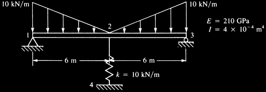
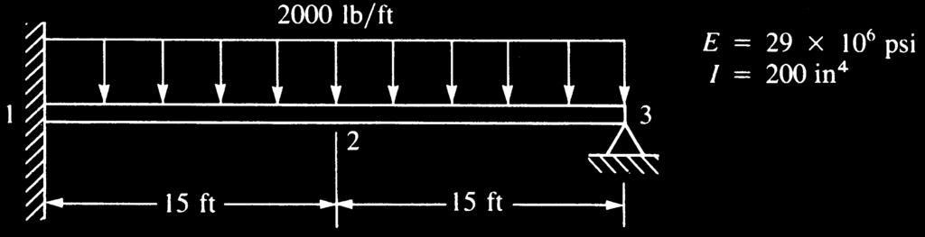
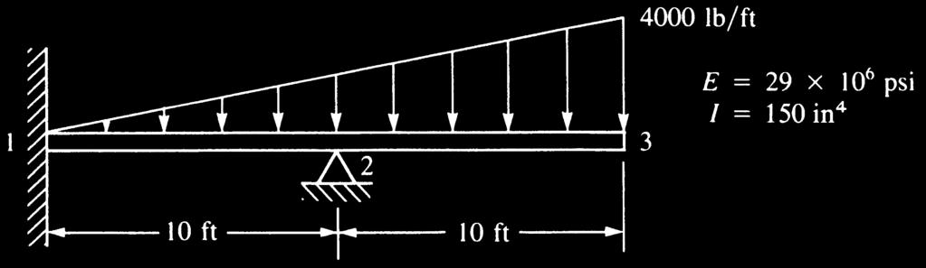
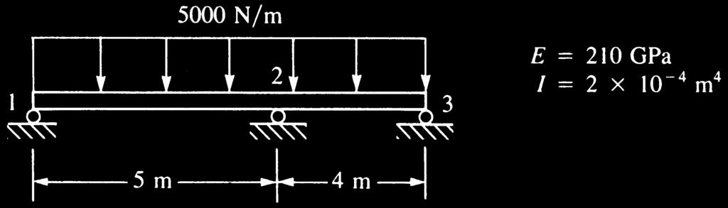
58 d 4 Development of Beam Equations Figure P4 Figure P4 1 Figure P4 Figure P4 Figure P4 4

59 Problems d For the beams shown in Figures P4 5 P4, determine the maximum deflection and maximum bending stress. Let E ¼ GPa or 1 psi for all beams as appropriate for the rest of the units in the problem. Let c be the half-depth of each beam. w = 1 kn m kn m A B C 4 m 4 m c =.5m, I = 1 1 m 4 Figure P4 5 A B C 1 m m I I c =.5m, I = 5(1 ) m 4 Figure P4 75 k A B C kip ft D A B 5 kn m C 15 ft 15 ft ft I I c = 1 in., I = 5 in. 4 1 m 5 m c =.m, I = 7 1 m 4 Figure P4 7 Figure P4 A 1.5 kip ft B 1 ft 1 ft c = 1 in., I = 4 in. 4 C 1 m m I I Figure P4 Figure P4 For the beam design problems shown in Figures P4 1 through P4, determine the size of beam to support the loads shown, based on requirements listed next to each beam. 4.1 Design a beam of ASTM A steel with allowable bending stress of 1 MPa to support the load shown in Figure P4 1. Assume a standard wide flange beam from Appendix F or some other source can be used. w = kn/m A 1 kn m B 1 kn c =.m, I = 7 1 m 4 C Figure P4 1 4 m 4 m

60 1 d 4 Development of Beam Equations 4. Select a standard steel pipe from Appendix F to support the load shown. The allowable bending stress must not exceed 4 ksi, and the allowable deflection must not exceed L/ of any span. 5 lb 5 lb 5 lb ft ft ft Figure P4 4. Select a rectangular structural tube from Appendix F to support the loads shown for the beam in Figure P4. The allowable bending stress should not exceed 4 ksi. 1 kip ft ft Figure P4 4.4 Select a standard W section from Appendix F or some other source to support the loads shown for the beam in Figure P4 4. The bending stress must not exceed 1 MPa. kn/m m m m Figure P For the beam shown in Figure P4 5, determine a suitable sized W section from Appendix F or from another suitable source such that the bending stress does not exceed 15 MPa and the maximum deflection does not exceed L/ of any span. 7 kn 7 kn 17 kn.5 m.5 m 5 m 1 m 1 m Figure P4 5

61 Problems d For the stepped shaft shown in Figure P4, determine a solid circular cross section for each section shown such that the bending stress does not exceed 1 MPa and the maximum deflection does not exceed L/ of the span. kn A B C D E Figure P4 m m m m 4.7 For the beam shown in Figure P4 7 subjected to the concentrated load P and distributed load w, determine the midspan displacement and the reactions. Let EI be constant throughout the beam. Figure P4 7 Figure P4 4. For the beam shown in Figure P4 subjected to the two concentrated loads P, determine the deflection at the midspan. Use the equivalent load replacement method. Let EI be constant throughout the beam. 4. For the beam shown in Figure P4 subjected to the concentrated load P and the linearly varying line load w, determine the free-end deflection and rotation and the reactions. Use the equivalent load replacement method. Let EI be constant throughout the beam. Figure P4 Figure P For the beams shown in Figures P4 4 P4 4, with internal hinge, determine the deflection at the hinge. Let E ¼ 1 GPa and I ¼ 1 4 m 4.

62 1 d 4 Development of Beam Equations Figure P4 41 Figure P Derive the stiffness matrix for a beam element with a nodal linkage that is, the shear is at node i, but the usual shear and moment resistance are present at node j (see Figure P4 4). Figure P Develop the stiffness matrix for a fictitious pure shear panel element (Figure P4 44) in terms of the shear modulus, G the shear web area, A W, and the length, L. Notice the Y and v are the shear force and transverse displacement at each node, respectively. Given 1Þ t ¼ G g ; Þ Y ¼ t Aw ; Þ Y 1 þ Y ¼ ; 4Þ g ¼ v v 1 L L L, 1 Y Y Y 1, 1 Y Figure P4 44 Positive node force sign convention Element in equilibrium (neglect moments) 4.45 Explicitly evaluate p p of Eq. (4.7.15); then differentiate p p with respect to ^d 1y ; ^f 1 ; ^d y, and ^f and set each of these equations to zero (that is, minimize p p ) to obtain the four element equations for the beam element. Then express these equations in matrix form. 4.4 Determine the free-end deflection for the tapered beam shown in Figure P4 4. Here IðxÞ ¼I ð1 þ nx=lþ where I is the moment of inertia at x ¼. Compare the exact beam theory solution with a two-element finite element solution for n ¼. Figure P4 4 Figure P4 47