cost733class-1.2 User guide

Transcription

1 cost733class-1.2 User guide Andreas Philipp 1, Christoph Beck 1, Pere Esteban 5,6, Frank Kreienkamp 2, Thomas Krennert 9, Kai Lochbihler 1, Spyros P. Lykoudis 3, Krystyna Pianko-Kluczynska 8, Piia Post 7, Domingo Rasilla Alvarez 10, Arne Spekat 2, and Florian Streicher 1 1 University of Augsburg, Germany 2 Climate and Environment Consulting Potsdam GmbH, Germany 3 Institute of Environmental Research and Sustainable Development, National Observatory of Athens, Greece 5 Group of Climatology, University of Barcelona, Spain 6 Institut d Estudis Andorrans (CENMA/IEA), Principality of Andorra 7 University of Tartu, Estonia 8 Institute of Meteorology and Water Management, Warsaw, Poland 9 Zentralanstalt fuer Meteorologie und Geodynamik, Vienna, Austria 10 University of Cantabria, Santander, Spain 02/10/2014

2

3 Contents 1 Introduction 1 2 Installation Getting the source code Using configure and make configure make Manual compilation as an alternative Troubleshooting For configure For make For runtime problems Getting started Principal usage Quick start Creating classifications Evaluating classifications Comparing classifications Assignment to existing classifications Rather simple (pre)processing Help listing Data input Foreign formats ASCII data file format COARDS NetCDF data format GRIB data format Other data formats Self-generated formats Binary data format Catalog files Files containing class centroids

4 4.3 Specifying data input and preprocessing Specification flags Flags for data set description Flags for spatial data Selection Flags for data Preprocessing Flags for data post processing Options for selecting dates Using more than one data set Options for overall PCA preprocessing of all data sets together Examples Simple ASCII data matrix ASCII data file with date columns NetCDF data selection Date selection for classification and centroids Data output The classification catalog Centroids or type composites Output on the screen Output of the input data Output of indices used for classification Opengl graphics output Classification methods Methods using predefined types INT interval BIN binclass GWT prototype - large scale circulation types GWTWS gwtws - large scale circulation types LIT lit - litynski threshold based method JCT jenkcol - Jenkinson-Collison Types WLK wlk - automatic weather type classification according to German metservice Methods based on Eigenvectors PCT tpca - t-mode principal component analysis using oblique rotation PTT tpcat - t-mode principal component analysis using orthogonal rotation PXE pcaxtr - the extreme score method KRZ kruiz - Kruizingas PCA-based types Methods using the leader algorithm LND lund - the Lund-method KIR kh - Kirchhofer

5 6.3.3 ERP erpicum HCL hclust - Hierarchical Cluster analysis Optimization algorithms KMN kmeans - conventional k-means with random seeds CAP pcaca - k-means of time filtered PC-scores and HCL starting partition CKM ckmeans - k-means with dissimilar seeds DKM dkmeans - a variant of ckmeans PXK pcaxtrkm - k-means using PXE starting partitions SAN sandra - simulated annealing and diversified randomization SOM som - self organizing (feature) maps (neural network according to Kohonen) KMD kmedoids - partitioning around medoids Random classifications RAN random RAC randomcent Assignments to existing classifications ASC assign CNT centroid Evaluation of classifications EVPF evpf - explained variation and pseudo F value ECV exvar WSDCIM wsdcim - Within-type standard deviation and confidence interval of the mean DRAT drat - Ratio of distances within and between circulation types FSIL fsil - Fast Silhouette Index SIL sil - Silhouette Index BRIER brier - Brier Score Comparison of classifications CPART cpart - Catalog comparison Miscellaneous functions AGG agg - Aggregation COR cor - Correlation SUB substitute - Substitute Visualization Development Implementing a new subroutine

6 12.2 Packing the directory for shipping Use of variables in the subroutine Using the input data from datainput.f The gnu autotools files References 103

7 1 Introduction 1 1 Introduction cost733class is a FORTRAN software package focused on creating and evaluating weather and circulation type classifications utilizing various different methods. The name refers to COST Action 733 which has been an initiative started in the year 2005 within the ESSEM (Earth System Science and Environmental Management) domain of the COST (European Cooperation in Science and Technology) framework. The topic of COST 733 is "Harmonisation and Applications of Weather Type Classifications for European regions". cost733class is released under GNU General Public License v3 (GPL) and freely available.

8 2 Installation 2 2 Installation The software is developed on Unix/Linux operating systems, however it may possible to compile and run it on other operating systems too, although some features may not work. At the time of writing this affects the NetCDF and grib data format and the OpenGL visualization, which are not necessary to run the program. 2.1 Getting the source code When you read this, you might have downloaded the software package and unpacked it already. However here is the way how to get and compile the software: To download direct your web browser to: http : / / c o s t c l a s s. geo. uni augsburg. de/ c o s t c l a s s 1.2 Here you will find instructions how to download the source code by SVN or how to get a tar package. If you have the tar-package unpack the bzip2 compressed tar-file e.g. by: t a r x v f j c o s t c l a s s 1.2 _RC_revision??. t a r. bz2 where?? stands for the svn version number. Change into the new directory: cd c o s t c l a s s Using configure and make The next step is to compile the source code to generate the executable called cost733class. For this you need to have a C and a FORTRAN90 compiler installed on your system. The compiler reads the source code from the src directory and generates the executable src/cost733class in the same directory which can be started on the command line of a terminal. In order to prepare the compilation process for automatic execution, so called Makefiles are generated by a script called configure. The configure script checks whether everything (tools, libraries, compilers) which is needed for compilation is installed on your system. If configure stops with an error, you have to install the package it is claiming about (see troubleshooting) and rerun configure until it is happy and creates the Makefiles. The package include some example shell scripts containing the command to configure and make the software in one step:

9 2 Installation 3 compile_gnu_debug.sh: this script uses the GNU Linux compilers gcc, gfortran and c++ to compile the software with NetCDF support but without GRIB and OpenGL support. Debugging information will be given in case of software errors. compile_gnu_debug_opengl.sh: this script additionally includes OpenGL support for visualization. compile_gnu_debug_grib.sh: this script additionally includes grib support. compile_gnu_debug_omp.sh:this script additionally includes compiler options to run parts of the code in parallel. compile_intel_omp.sh: this script uses the intel compiler suite. In order to execute these scripts you type e.g.:. / compile_gnu_debug_opengl. sh or sh compile_gnu_debug_opengl. sh These scripts can be easily copied and modified to save compiler options which are often needed. However it is also possible to run the two commands configure and make manually one after the other, as described in the following configure The configure script tries to guess which compilers should be used, however it is advisable to specify the compilers by setting the FC= and CC= flags. E.g. if you want to use the GNU compilers gfortran and gcc say:. / c o n f i g u r e FC=g f o r t r a n CC=gcc or if the intel compilers should be used:. / c o n f i g u r e FC=i f o r t CC=i c c Note that the FORTRAN and C compilers should be able to work together, i.e. the binaries must be compatible. This is not always the case e.g. when mixing other and GNU compilers (depending on versions). Also you can use some special compiler options, e.g. for running parts of the classifications in parallel:. / c o n f i g u r e FC=i f o r t CC=i c c FCFLAGS=" p a r a l l e l openmp" In the same manner options for the C-compiler can be set by the CCFLAGS="..." option. By default cost733class compiles with netcdf, GRIB and OpenGL support. Further options for the configure script control and disable special features of the package:

10 2 Installation 4. / c o n f i g u r e d i s a b l e g r i b switches off the compilation of the GRIB_API, thus grib data can t be read by the software.. / c o n f i g u r e d i s a b l e opengl switches off the compilation of routines which visualize some of the classification processes like SOM, SAN or CKM. This feature is working only for unix systems with opengl-development packages (gl-dev glut-dev x11-dev) installed make The compiling process itself is done by the tool called make: make If everthing went well, you will find the executable cost733class in the src directory. Check it by running the command: s r c / c o s t c l a s s If you have administrator privileges on your system you can install the executables into /usr/local/bin. Note that the NetCDF tools coming along with cost733class are also installed there. sudo make su i n s t a l l Alternatively you can copy only the executable to any bin directory to have it in your command search path: sudo copy s r c / c o s t c l a s s / usr / l o c a l / bin That s it, you can now start to run classifications, which of course needs some input data describing the atmospheric state of each time step (i.e. object) you want to classify. You can now try with the next chapter (Quick start) or look into the Data input chapter. 2.3 Manual compilation as an alternative Within the package directory there is a batch file called compile_mingw.bat for Windows. This script file contains the direct compile command for the gfortran and g95 compiler without any dependencies to any libraries. It can be used if no NetCDF input is needed or if there are troubles compiling the NetCDF package.

11 2 Installation Troubleshooting For configure If configure claims about something missing or a wrong version number, you have to install or update the concerning software packages. For Debian and Ubuntu systems that s rather easy. First you have to find out the official name of the package which contains the files configure was claiming about. Here you can use the tool apt-file which must be installed first, updated and run: sudo apt get i n s t a l l apt f i l e apt f i l e update apt f i l e s e a r c h <filename > It will then print the name of the package in the first column and you can use it to install the missing package: sudo apt get i n s t a l l <package> For make If the following error message appears: C a t a s t r o p h i c e r r o r : could not s e t l o c a l e "" to a l l o w p r o c e s s i n g o f multibyte c h a r a c t e r s setting the environment variable LANG to C export LANG=C in the shell you use for compilation will fix it For runtime problems Some methods need a lot of RAM and maybe more than is available. If this is the case you can try to enlarge stack size each time you run the software by u l i m i t s u n l i m i t e d If the following error or a similar error occurs: g l i b c d e t e c t e d double f r e e or c o r r u p t i o n (! prev ) : 0 x this is probably due to differing compiler/library versions. You can try to get rid of it by: export MALLOC_CHECK_=0

12 2 Installation 6 If compiled with grib support and running cost733class results in the following error: GRIB_API ERROR : Unable to f i n d boot. d e f grib_context. c at l i n e : a s s e r t i o n f a i l u r e A s s e r t ( 0 ) Aborted one has to define the path to the so called grib definitions. In an Unix environment something like export GRIB_DEFINITION_PATH="/PATH/ c o s t c l a s s 1.2/ grib_api / d e f i n i t i o n s " should do it. Use absolute paths! Depending on the processor type and data size method SAN and SOM may run for several hours up to days. This is no bug!

13 3 Getting started 7 3 Getting started 3.1 Principal usage cost733class has been written to simplify and unify the generation of classification catalogs. It s functionality is controlled by command line arguments, i.e. options are given as key words after the command which is entered into a terminal or console providing a command prompt. The command line interface (CLI) makes the software suitable for shell scripts and can easily run on compute servers or clusters in the background. Recently a graphical user interface (GUI) has been added by using the OpenGL menu functions which is accessible by a right click into the OpenGL window, however it is not very intuitive yet. Therefore the documentation will concentrate on the CLI interface. If you type src/cost733class just after the compilation process you will see the output of the -help function. In order to run a classification, you have to provide command line arguments for the program, i.e. you have to type expressions behind the cost733class command which are separated by blanks (" "). The program will scan the command line and recognize all arguments beginning with a "-", several of which have to be followed by another expression. All expressions have to be separated by one or more blanks, which is the reason that in between any expression (e.g. a file name) no blank is allowed. Also all expressions have to be written in lower/upper case letters if said so in the -help output. Command lines can be rather simple, however some methods and the data configurations can be complex, thus that the command line gets longer and longer the more you want to fine tune your classification. In this case, and especially if just variations of a classifications should be run one after another, it can be useful to use shell scripts to run the software which will be explained below. In order to understand which options play a role for which part of the classification it is helpful to distinguish between options relevant for the data input and preprocessing and options relevant for the routines itself. In order to better understand how the software works and how it can be used, the workflow is briefly described in the following: In the first step the command line arguments are analyzed (subroutine arguments()). For each option default values are set within the program, however they are changed if respective options are provided by the user. The next step is to evaluate the data which should be read from a file, especially the size of the data set has to be determined here in order to reserve (allocate) computer memory for it. Then the data are read into a preliminary array (RAWDAT) and eventually are preprocessed (selected, filtered, etc.) before they are put into the final, synchronized, DAT array which is used by the

14 3 Getting started 8 methods. In some cases (depending on the classification/evaluation operation) existing catalogs have to read. This is done in the next step by the subroutine classinput(). Afterwards the subroutine for the desired operation is called. If this subroutine finished with a new catalog, it is written to a classification catalogue file (*.cla) and the program ends. Other routines e.g. for comparison or evaluation of classification catalogs might just produce screen output. 3.2 Quick start As an requirement to write complex commands it is necessary to understand the basic synopsis of cost733class. There are several different use cases in which cost733class can be used: 1. Creation of classifications of any numerical data following an entity-attribute-value model (main purpose of cost733class). For more information about the data model used by cost733class see section Evaluation of such classifications 3. Comparison of such classifications 4. Assignment of existing classifications to new data 5. Rather simple data (pre)processing All of these use cases require different commands following different structures. Therefor the next sections give brief instructions on how to use cost733class for each of these five cases Creating classifications For the creation of classifications a basic command follows the scheme: c o s t c l a s s dat <s p e c i f i c a t i o n > [ dat <s p e c i f i c a t i o n >] met <method> [ n c l <i n t e g e r >] [ cnt <filename >] [ c l a < f i l e >] [ more method s p e c i f i c o p t i o n s ] Essential for a successful completion of each classification run is the -dat <specification> option which provides necessary information about the input data. For some methods it is possible to give more than one data specification option, for others it is prerequisite. Furthermore the classification method must be named by the -met <method> option. The number of classes can be specified with -ncl <integer>. The filenames for the output of the classification catalog and the corresponding class centroids can be defined by -cla <filename> and -cnt <filename>. Depending on the used classification method several other options can be provided by special options. For further documentation of these consult the relative section. Based on this the command for a classification with the method KMN may look like:

15 3 Getting started 9 c o s t c l a s s dat pth : s l p. dat n c l 9 met KMN c l a KMN_ncl9. c l a Evaluating classifications The basic scheme of an evaluation command is: c o s t c l a s s dat <s p e c i f i c a t i o n > [ dat <s p e c i f i c a t i o n >] c l a i n <s p e c i f i c a t i o n > met <method> [ idx <filename >] [ more method s p e c i f i c o p t i o n s ] The most important difference to a classification run is the -clain <specification> option. It defines the path to an existing classification catalog file and is mandatory for all evaluation methods. The desired evaluation method must be chosen by the -met <method> option. The results are written to one or more files for which the base name can be given by the -idx <filename> option. Analogous to the previous command every method has its additional options which are explained in the corresponding sections below. At least one -dat <specification> option describes the data one wants to evaluate with. A cost733class run which evaluates the classification generated by the previous command using the Brier Score would be: c o s t c l a s s dat pth : s l p. dat c l a i n pth : KMN_ncl9. c l a met BRIER idx brier_kmn_ncl9. t x t Comparing classifications Comparing two or more classifications is rather easy: c o s t c l a s s c l a i n <s p e c i f i c a t i o n > [ c l a i n <s p e c i f i c a t i o n >] met <method> [ idx <filename >] [ more method s p e c i f i c o p t i o n s ] The only difference to an evaluation and classification run is the absence of the -dat <specification> option. Instead at least two classification catalogs (more than one per file are possible) must be provided. A comparison of two partitions based on different methods could be done with: c o s t c l a s s c l a i n pth : DKM_ncl9. c l a c l a i n pth : KMN_ncl9. c l a met CPART idx KMN_DKM_ncl9_compared. t x t Assignment to existing classifications Assignments to existing classifications can be done on two different bases: 1. for a given classification catalog 2. for predefined class centroids

16 3 Getting started 10 In both cases one has to provide and describe data which is then assigned to an existing classification. Other required cost733class options differ in both cases. Please refer to the corresponding sections below Rather simple (pre)processing Beyond the use cases mentioned above there are a few methods in cost733class which process input data in a different way. They are grouped together under the term miscellaneous functions. Furthermore it is possible to just preprocess input data without calling a distinctive method. c o s t c l a s s dat <s p e c i f i c a t i o n > [ o p t i o n s f o r s e l e c t i n g d a t e s ] w r i t e d a t <filename > In this case data output can be accomplished by the -witedat <filename> option. There are several flags for preprocessing and spatial selection which are listed and described in the relative section. An example might be: c o s t c l a s s dat pth : s l p. dat lon : 10:30:2.5 l a t : 3 5 : 6 0 : 2. 5 f d t : : 1 : 1 : 1 2 l d t : : 1 2 : 3 1 : 1 2 ddt : 1d ano : 3 f i l : 30 per : 1 : 1 : 1 2, : 1 2 : 3 1 : 1 2, 1 d w r i t e d a t output. bin Note that here the output data are unformatted binary files (extension: bin). These files can be read by cost733class in a subsequent run. This proceeding can be very helpful if many runs of cost733class are planned. 3.3 Help listing If you run the cost733class command without any command line argument (or with the -help option) you should see the following help text, giving a brief description of the various options: USAGE:.. / s r c / c o s t c l a s s dat <s p e c i f i c a t i o n > [ dat <s p e c i f i c a t i o n >] [ o p t i o n s ] OPTIONS: INPUT DATA: dat <char> : s p e c i f i c a t i o n o f input data. More than one dat arguments : are allowed to combine data o f same sample s i z e but from : d i f f e r e n t f i l e s i n d i f f e r e n t formats. : <char> c o n s i s t s o f v a r i o u s s p e c i f i c a t i o n s s e p a r a t e d by the : c h a r a c t e or one or more blanks : o f v a r i a b l e > f o r fmt : n e t c d f t h i s must be the : v a r i a b l e name i n the n e t c d f f i l e f o r input data f i l e > : i n c a s e o f n e t c d f i t may i n c l u d e "?" symbols to be : r e p l a c e d by numbers given by the f d t : and l d t : f l a g s. a s c i i " or " n e t c d f " or " g r i b"> d e f a u l t a s c i i

17 3 Getting started 11 : I f f i l e name ends with ". nc" n e t c d f i s assumed ; : f o r ". g r i b /. grb /. gribx /. grbx" (X= [ 1, 2 ] ) g r i b i s assumed. : a s c i i : ( d e f a u l t ) a s c i i f i l e with one l i n e per day ( o b j e c t : to c l a s s i f y ) and one column per v a r i a b l e ( parameter : d e f i n i n g the o b j e c t s ) the columns have to be d e l i m i t e d : by one or more blanks. The number o f o b j e c t s and : v a r i a b l e s i s scanned by t h i s program on i t s own. : n e t c d f : data i n s e l f d e s c r i b i n g n e t c d f format. : time and g r i d i s scanned a u t o m a t i c a l l y. : g r i b : data i n s e l f d e s c r i b i n g format. : time and g r i d i s scanned a u t o m a t i c a l l y. 4> ( number o f l e a d i n g date columns : year, month, : day, hour i n a s c i i f i l e ) f i r s t date i n d a t a s e t ( d e s c r i p t i o n ) l a s t date i n d a t a s e t ( d e s c r i p t i o n ) int ><y m d h> time s t e p i n data s e t i n years, months, : days or hours l i s t o f months> months i n data set, e. : 1 : 2 : 1 2 >:<maxlon>:< d i f l o n > l o n g i t u d e d e s c r i p t i o n :< minlat >:<maxlat >:< d i f l a t > l a t i t u d e d e s c r i p t i o n :<minlon >:<maxlon>:< d i f l o n > l o n g i t u d e s e l e c t i o n :< minlat >:<maxlat >:< d i f l a t > l a t i t u d e s e l e c t i o n :< l e v e l between 1000 and 10> s e l e c t i o n i n t e g e r > area w e i g h t i n g 1=cos ( l a t i t u d e ), : 2=s q r t ( cos ( l a t i t u d e ) ), : 3= c a l c u l a t e d weights by area o f g r i d box which i s the same : as cos ( l a t i t u d e ) o f option 1 :< f l o a t > s c a l i n g o f data v a l u e s :< f l o a t > o f f s e t value to add a f t e r s c a l i n g int > o b j e c t ( row wise ) n o r m a l i s a t i o n : : 1=c e n t e r i n g,2= std ( sample ),3= std ( p o p u l a t i o n ) int > v a r i a b l e ( column wise ) n o r m a l i s a t i o n : : done a f t e r s e l e c t i o n o f time s t e p s : : 1=c e n t e r i n g, 2= std ( sample ), 3= std ( p o p u l a t i o n ) : done b e f o r e s e l e c t i o n o f time s t e p s : : 1=c e n t e r i n g,2= std ( sample ),3= std ( p o p u l a t i o n ) : 11= c e n t e r i n g f o r days o f year, : 12= std f o r days ( sample ),13= std ( p o p u l a t i o n ) : 21= c e n t e r i n g f o r months, : 22= std f o r months ( sample ), : 23= std ( p o p u l a t i o n ) : 31= c e n t e r i n g on monthly mean ( running 31 day window ), : 32= std f o r months ( sample ) ( running 31 day window ), : 33= std ( p o p u l a t i o n ) ( running 31 day window ) f i l :< i n t e g e r > g a u s s i a n time f i l t e r int >0 > low pass : int <0 > high pass f l o a t i n t e g e r > PCA o f parameter data s e t : : i f <f l o a t >: f o r r e t a i n i n g e x p l a i n e d v a r i a n c e : f r a c t i o n, i f <int >: number o f PCs f l o a t i n t e g e r > but with w e i g h t i n g by : e x p l a i n e d v a r i a n c e sequence l e n g t h f o r e x t e n s i o n > w e i g h t i n g f a c t o r > f i l e name> f i l e name to w r i t e c e n t r o i d / composite : v a l u e s to i f e x t e n s i o n = ". nc" i t i s n e t c d f format, : a s c i i o t h e r w i s e ( with c o o r d i n a t e s f o r. txt, without : f o r. dat ). readncdate : read the date o f o b s e r v a t i o n s from n e t c d f time v a r i a b l e r a t h e r : than c a l c u l a t i n g i t from " a c t u a l range " a t t r i b u t e o f the : time v a r i a b l e ( s l o w s down the data input but can o v e r r i d e : buggy a t t r i b u t e e n t r i e s as e. g i n s l p nc ).

18 3 Getting started 12 per <char> : p e r i o d s e l e c t i o n, <char> i s e. g : 1 : 1 : 1 2, : 1 2 : 3 1 : 1 2, 1 d mon <char> : l i s t o f months to c l a s s i f y : MM,MM,MM,... : e. g. : mon 12,01,02 c l a s s i f i e s w i nter data ( d e f a u l t i s a l l : months ), only a p p l i e s i f per i s d e f i n e d! mod : LIT : s e t a l l months to be 30 days long ( r e l e v a n t f o r met l i t ) d l i s t <char> : l i s t f i l e name f o r s e l e c t i n g a s u b s e t o f d a t e s w i thin the : given p e r i o d f o r c l a s s i f i c a t i o n. Each l i n e has to hold one : date i n form : "YYYY MM DD HH" f o r year, month, day, hour. : I f hour, day or month i s i r r e l e v a n t p l e a s e p r o v i d e the c o n s t a n t : dummy number 0 0. cat <spec> : c l a s s i f i c a t i o n c a t a l o g input, where <spec> c o n s i s t s o f the f o l l o w i n g f l a g s f o r f i l e f i r s t l a s t time step, e. g. "@ddt : 1 d" f o r one o f date l i s t o f months> e. g. "@mdt: 0 1, 0 2, 1 2 " catname <char> : f i l e with as many l i n e s as c a t a l o g s read i n by " cat ", each l i n e c o n t a i n s the name o f the c a t a l o g o f the c o r r e s o n d i n g column i n the c a t a l o g f i l e. c n t i n <char> : c e n t r o i d input f i l e f o r met ASS and ASC pca <f l o a t i n t e g e r >: PCA o f input data a l l t o g e t h e r : : i f <f l o a t >: f o r r e t a i n i n g e x p l a i n e d v a r i a n c e f r a c t i o n : i f <int >: number o f PCs pcw <f l o a t i n t e g e r >: PCA o f input data, PCs weighted by e x p l a i n e d v a r i a n c e : : i f <f l o a t >: f o r r e t a i n i n g e x p l a i n e d v a r i a n c e f r a c t i o n : i f <int >: number o f PCs OUTPUT: c l a < c l a f i l e > : name o f c l a s s i f i c a t i o n output f i l e ( c o n t a i n s number o f c l a s s : f o r each o b j e c t i n one l i n e ). : d e f a u l t =./<basename ( d a t f i l e )>_<method>_ncl<int >. c l a mcla < c l a f i l e >: m u l t i p l e c l a s s i f i c a t i o n output f i l e. Some methods g e n e r a t e : more than one ( nrun ) c l a s s i f i c a t i o n and s e l e c t the b e s t. : o p t ion mcla < f i l e > makes them w r i t i n g out a l l. skipempty <F T> : s k i p empty c l a s s e s i n the numbering scheme? T=yes, F=no : D e f a u l t i s "T" w r i t e d a t <char >: w r i t e p r e p r o c e s s e d input data i n t o f i l e name <char> d c o l <int > : w r i t e datum columns to the c l a o u t p u t f i l e : : <int >=1: year, <int >=2: year, month, <int >=3: year, month, day, : <int >=4: year, month, day, hour cnt <char> : w r i t e c e n t r o i d data to f i l e named <char> ( c o n t a i n s composites : o f the input data f o r each type i n a column ). sub <char> : method SUB: w r i t e s u b s t i t u t e data to f i l e named <char> agg <char> : method AGG: w r i t e aggregated data to f i l e named <char> idx <char> : w r i t e index data used f o r c l a s s i f i c a t i o n to f i l e named : <char >.<ext>

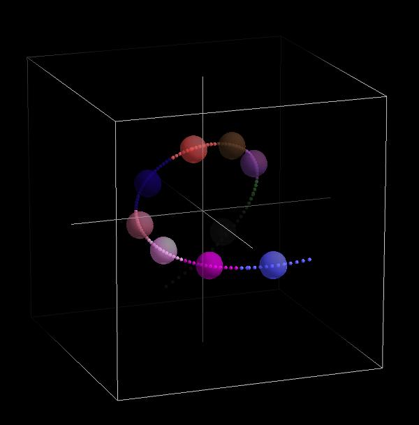
19 3 Getting started 13 : the type o f the i n d i c e s dependes on the method ( e. g. s c o r e s : and l o a d i n g f o r PCT) opengl : t h i s switch a c t i v a t e s the 3D v i s u a l i s a t i o n output c a l l s f o r : the f o l l o w i n g methods : : SOM c r i t 2, SAN, CKM. : This i s only working without p a r a l l e l i z a t i o n and probably on : unix / l i n u x systems : The s o f t w a r e c o m p i l a t i o n has to be c o n f i g u r e d by : ". / c o n f i g u r e enable opengl ". g l j p e g : i n c o n j u n c t i o n with opengl t h i s switch produces s i n g l e : jpg images which can be used to c r e a t e animations. glwidth : width o f opengl g r a p h i c s window ( d e f a u l t =800) g l h e i g h t : h e i g h t o f opengl g r a p h i c s window ( d e f a u l t =800) g l p s i z e : s i z e o f data p o i n t s ( d e f a u l t =0.004D0) g l c s i z e : s i z e o f c e n t r o i d p o i n t s ( d e f a u l t =0.03D0) g l x a n g l e <r e a l > : a n g l e to t i l t view on data cube ( d e f a u l t = 60.D0) g l y a n g l e <r e a l > : a n g l e to t i l t view on data cube ( d e f a u l t = 0. D0) g l z a n g l e <r e a l > : a n g l e to t i l t view on data cube ( d e f a u l t = 3 5.D0) g l s t e p : time s t e p p i n g ( d e f a u l t =10) g l p a u s e : pause l e n g t h ( d e f a u l t =1) glbackground <int > : background c o l o r : 0=black ( d e f a u l t ), 1=white g l r o t a n g l e <angle > : r o t a t i o n a n g l e s t e p f o r s p i n n i n g cube METHODS: met <method> : method : : NON none : j u s t read ( and w r i t e ) data and e x i t : INT i n t e r v a l BIN : c l a s s i f y i n t o i n t e r v a l s o f v a r i a b l e s v a r : GWT prototype : prototype g r o s s w e t t e r l a g e n, c o r r e l a t i o n based, : r e s u l t i n g i n 26 types : GWTWS gwtws : based on GWT ( above ) u s i n g 8 types, : r e s u l t i n g i n 11 types : LIT l i t : l i t y n s k i t h r e s h o l d s, one c i r c u l a t i o n f i e l d, : dates, n c l = : JCT j e n k c o l l : Jenkinson C o l l i s o n scheme : WLK wlk : t h r e s h o l d based u s i n g p r e s s u r e, wind, : temperature and humidity : PCT TPC tmodpca : t mode p r i n c i p a l component a n a l y s i s o f 10 data : s u b s e t s, o b l i q u e r o t a t i o n : PTT TPT tmodpcat : t mode p r i n c i p a l component a n a l y s i s, : varimax r o t a t i o n : PXE pcaxtr : s mode PCA u s i n g high p o s i t i v e and n e g a t i v e : s c o r e s to c l a s s i f y o b j e c t s : KRZ k r u i z : Kruizinga PCA scheme

20 3 Getting started 14 : LND lund : count most f r e q u e n t s i m i l a r p a t t e r n s ( t h r e s ) : KIR k i r c h h o f e r : count most f r e q u e n t s i m i l a r p a t t e r n s ( t h r e s ) : ERP erpicum : count most f r e q u e n t s i m i l a r p a t t e r n s, a n g l e : d i s t a n c e, a d j u s t i n g t h r e s h o l d s : HCL h c l u s t : h i e r a r c h i c a l c l u s t e r a n a l y s i s ( Murtagh 1986), : s e e parameter c r i t! : KMN kmeans : k means c l u s t e r a n a l y i s ( Hartigan /Wong 1979 : a lgorithm ) : CKM ckmeans : l i k e dkmeans but e v e n t u a l l y s k i p s s m a l l c l u s t e r s : <5% p o p u l a t i o n : DKM dkmeans : k means ( simple a l g o r i t h m ) with most d i f f e r e n t : s t a r t p a t t e r n s : SAN sandra : simulated a n n e a l i n g and d i v e r s i f i e d randomisation : c l u s t e r i n g : SOM som : s e l f o r g a n i s i n g maps ( Kohonen n e u r a l network ) : KMD kmedoids : P a r t i t i o n i n g Around Medoids : RAN random : j u s t produce random c l a s s i f i c a t i o n c a t a l o g u e s : RAC randomcent : determine c e n t r o i d s by random and a s s i g n o b j e c t s : to i t. : ASC a s s i g n : no r e a l method : j u s t a s s i g n data to given : c e n t r o i d s provided by c n t i n : SUB s u b s t i t u t e : s u b s t i t u t e c a t a l o g numbers by v a l u e s given i n a c n t i n f i l e : : AGG a g g r e g a t e : b u i l d s e a s o n a l v a l u e s out o f d a i l y or monthly v a l u e s. : : COR c o r r e l a t e : c a l c u l a t e c o r r e l a t i o n m e t r i c s comparing the input data v a r i a b l e s. : : CNT c e n t r o i d : c a l c u l a t e c e n t r o i d s o f given c a t a l o g ( c l a i n ) : and data ( s e e dat ), s e e a l s o cnt : ECV exvar : e v a l u a t i o n o f c l a s s i f i c a t i o n s by Explained : C l u s t e r Variance ( s e e c l a i n c r i t ) : EVPF evpf : e v a l u a t i o n i n terms o f e x p l a i n e d v a r i a t i o n : and pseudo F value ( c l a i n ) : WSDCIM wsdcim : e v a l u a t i o n i n terms o f within type SD and : c o n f i d e n c e i n t e r v a l ( c l a i n ) : FSIL f s i l : e v a l u a t i o n i n terms o f the Fast S i l h o u e t t e : Index ( c l a i n ) : SIL s i l : e v a l u a t i o n i n terms o f the S i l h o u e t t e Index : ( c l a i n ) : DRAT drat : e v a l u a t i o n i n terms o f the d i s t a n c e r a t i o : w ithin and between c l a s s e s ( c l a i n ) : CPART c p a r t : c a l c u l a t e comparison i n d i c e s f o r >= 2 given : p a r t i t i o n s ( c l a i n ) : ARI randindex : c a l c u l a t e only ( a d j u s t e d ) Rand i n d i c e s f o r : two or more p a r t i t i o n s given by c l a i n c r i t <int > : INT i n t e r v a l : : 1 = c a l c u l a t e t h r e s h o l d s as i th p e r c e n t i l e where i=c l 1/ n c l : 2 = b i n s c e n t e r e d around the mean value : 3 = bin s i z e i s the data range / ncl, the b i n s are not c e n t e r e d. : 4 = 2 b i n s d i v i d e d by t h r e s <r e a l > f o r s v a r <int >. : 5 = as 4 but t h r e s h o l d i s i n t e r p r e t e d a p e r c e n t i l e (0 to 100). : HCL: ( h i e r a r c h i c a l c l u s t e r i n g ) : number o f c r i t e r i o n : : 1 = Ward s minimum v a r i a n c e method : 2 = s i n g l e l i n k a g e : 3 = complete l i n k a g e

21 3 Getting started 15 : 4 = average l i n k a g e : 5 = Mc Quitty s method : 6 = median ( Gower s ) method : 7 = c e n t r o i d method : GWT: : 1 = raw c o e f f i c i e n t s f o r v o r t i c i t y ( d e f a u l t ) : 2 = normalized v o r t i c i t y c o e f f i c i e n t s : GWTWS: : 1 = c l a s s i f i c a t i o n based on a b s o l u t v a l u e s ( d e f a u l t ) : 2 = c l a s s i f i c a t i o n based on p e r c e n t i l e s : ECV: : 1 = monthly normalized data ( d e f a u l t ) : 0 = raw data f o r c a l c u l a t i n g e x p l a i n e d c l u s t e r v a r i a n c e. : PCT: r o t a t i o n c r i t e r i a : : 1 = d i r e c t oblimin, gamma=0 ( d e f a u l t ) : WLK: : 0 = use raw c y c l o n i c i t y f o r d e c i d i n g a n t i c y c l o n i c or c y l o n i c ( d e f a u l t ) : 1 = use anomalies o f c y c l o n i c i t y : JCT : : 1 = c e n t e r e d c l a s s i f i c a t i o n g r i d with an extend o f 30 W E; 2 0 N S ( d e f a u l t ) : 2 = c l a s s i f i c a t i o n g r i d extended to data r e g i o n : SOM: : 1 = 1 d i m e n s i o n a l network topology : 2 = 2 d i m e n s i o n a l network topology : KMD: : 0 = use Chebychev d i s t a n c e d=max ( xa xb ) : 1 = use Manhattan d i s t a n c e d=sum ( xa xb ) : 2 = use Euclidean d i s t a n c e d=s q r t (sum ( ( xa xb ) 2) ) : p = use Minkovski d i s t a n c e o f o r d e r p : d=(sum ( xa xb p ) ) (1/ p ) : PXE/PXK: : 0 = only n o r m a l i z e p a t t e r n s f o r PCA ( o r i g i n a l ) : 1 = n o r m a l i z e p a t t e r n s and n o r m a l i z e g r i d p o i n t v a l u e s a f t e r w a r d s ( d e f a u l t ) : 2 = n o r m a l i z e p a t t e r n s and c e n t e r g r i d p o i n t v a l u e s a f t e r w a r d s : EVPF, WSDCIM, FSIL, SIL, DRAT: : 0 = e v a l u a t e on the b a s i s o f the o r i g i n a l data v a l u e s : 1 = e v a l u a t e on the b a s i s o f d a i l y anomaly v a l u e s : 2 = e v a l u a t e on the b a s i s o f monthly anomlay v a l u e s : BRIER : : 1 = q u a n t i l e to a b s o l u t v a l u e s ( d e f a u l t ) : 2 = q u a n t i l e to e u c l i d e a n d i s t a n c e s between p a t t e r n s t h r e s <r e a l > : KRC and LND: d i s t a n c e t h r e s h o l d to s e a r c h f o r key p a t t e r n s : d e f a u l t = 0. 4 f o r k i r c h h o f e r and 0. 7 f o r lund. : INT : t h r e s h o l d between b i n s. : WLK: f r a c t i o n o f g r i d p o i n t s f o r d e c i s i o n on main wind s e c t o r ( d e f a u l t =0.6) : PXE/PXK: t h r e s h o l d d e f i n i n g key group ( d e f a u l t =2.0) : BRIER : q u a n t i l e [ 0, 1 ] ( d e f a u l t =0.9) to d e f i n e extreme e v e n t s. An event i s : d e f i n e d when the e u c l i d e a n d i s t a n c e to the p e r i o d s / s e a s o n a l / monthly mean p a t t e r n : i s g r e a t e r than the given q u a n t i l e. I f <t h r e s > i s s i g n e d n e g a t i v e ( e. g. 0.8), : than e v e n t s are d e f i n e d i f s m a l l e r than the given q u a n t i l e. s h i f t : WLK: s h i f t 90 d egree wind s e c t o r s by 45 degree. D e f a u l t i s no s h i f t. n c l <int > : number o f c l a s s e s ( must be between 2 and 256) nrun <int > : number o f runs ( f o r SAN, SAT, SOM, KMN) f o r s e l e c t i o n o f b e s t r e s u l t.

22 3 Getting started 16 : C l u s t e r a n a l y s i s i s by d e s i g n an u n s t a b l e method f o r complex d a t a s e t s. : The more r e p e a t e d runs are used to s e l e c t the b e s t r e s u l t the more robust : i s the r e s u l t. SOM and SAN are d e s i g n e d to be much more robust than KMN. : d e f a u l t = nrun 1000 to produce r e l i a b l e r e s u l t s! s t e p <int > : SOM: number o f epochs a f t e r which neighbourhood r a d i u s i s to be reduced : For t r a i n i n g the neurons, a l s o neighboured neurons o f the winner neuron : i n the network map are a f f e c t e d and adapted to the t r a i n i n g p a t t e r n ( to a : lower d egree though ). The neighbourhood r a d i u s c o v e r s a l l neurons ( c l a s s e s : at the b e g i n n i n g and i s reduced during the p r o c e s s u n t i l only the winner neuron : i s a f f e c t e d. This slow d e c r e a s e h e l p s to overcome l o c a l minima i n the o p t i m i s a t i o n : f u n c t i o n. : d e f a u l t = s t e p 10 ( meaning a f t e r 10 epochs neighbourhood r a d i u s i s reduced : by one ). : WLK: number o f w i n d s e c t o r s : EVPF, WSDCIM, FSIL, SIL, DRAT, CPART: m i s s i n g value i n d i c a t o r f o r c a t a l o g u e data n i t e r <int > : SOM, SAN, PXE, PXK: maximum number o f epochs / i t e r a t i o n s to run : d e f a u l t s : : n i t e r 0 f o r pcaxtr means that only the f i r s t assignment to the pc c e n t r o i d s i s done. : f o r PXK n i t e r i s ( means k means i t e r a t i o n s ) : f o r SAN t h e r e i s no d e f a u l t f o r n i t e r ( i n f i n i t y ). Enable i t i f SAN ends up i n an e n d l e s s loop. temp <r e a l > : s imulated a n n e a l i n g s t a r t temperature ( f o r CND) : d e f a u l t = 1 c o o l <r e a l > : c o o l i n g r a t e ( f o r som & sandra ) : d e f a u l t = c o o l D0 ; s e t to D0 or c l o s e r to 1. D0 to enhance ( and slow down ). svar <int > : tuning parameter : INT : number o f v a r i a b l e /column to use f o r c a l c u l a t i n i n t e r v a l t h r e s h o l d s. alpha <r e a l > : tuning parameter : WLK: c e n t r a l weight f o r w e i g h t i n g mask ( d e f a u l t =3.D0) : EVPF, WSDCIM, FSIL, SIL, DRAT: s c a l e f a c t o r f o r e v a l u a t i o n data : BRIER : : i f < 0 => ( d e f a u l t ) use a l l v a l u e s ( c r i t 1) or p a t t e r n s ( c r i t 2) : i f >=0 => a value or p a t t e r n i s p r o c e s s e d only i f i t s e l f or mean ( p a t t e r n ) > alpha. : GWTWS: value / p e r c e n t i l e f o r low winds ( main t h r e s h o l d f o r types 9, 1 0, 1 1 ) beta <r e a l > : tuning parameter : WLK: middle zone weight f o r w e i g h t i n g mask ( d e f a u l t =2.D0) : EVPF, WSDCIM, FSIL, SIL, DRAT: o f f s e t value f o r e v a l u a t i o n data : GWTWS: value / p e r c e n t i l e f o r f l a t winds ( type 11) gamma <r e a l > : tuning parameter

23 3 Getting started 17 : WLK: margin zone weight f o r w e i g h t i n g mask ( d e f a u l t =1.D0) : WSDCIM: c o n f i d e n c e l e v e l f o r e s t i m a t i n g the c o n f i d e n c e i n t e r v a l o f the mean : GWTWS: value / p e r c e n t i l e f o r low p r e s s u r e ( type 9) d e l t a <r e a l > : tuning parameter : WLK: width f a c t o r f o r w e i g t h i n g zones ( nx d e l t a ny d e l t a ) ( d e f a u l t =0.2) : PXE/PXK: s c o r e l i m i t f o r o t h e r PCs to d e f i n e u n i q u e l y l e a d i n g PC ( d e f a u l t 1. 0 ) : GWTWS: value / p e r c e n t i l e f o r high p r e s s u r e ( type 10) lambda <r e a l > : tuning parameter : SAT: w e i g h t i n g f a c t o r f o r time c o n s t r a i n e d c l u s t e r i n g ( d e f a u l t =1.D0) d i s t <int > : d i s t a n c e m e tric ( not f o r a l l methods yet ) : : i f i n t > 0 : Minkowski d i s t a n c e o f o r d e r i n t (0=Chebychev ), : i f i n t = 1: 1 c o r r e l a t i o n c o e f f i c i e n t. nx <int > : KIR : number o f l o n g i t u d e s, needed f o r row and column c o r r e l a t i o n s : DRAT: d i s t a n c e measure to use (1= e u c l i d e a n d i s t a n c e, 2=pearson c o r r e l a t i o n ) ny <int > : KIR : number o f l a t i t u d e s wgttyp e u c l i d normal : a d j u s t weights f o r s i m u l a t i n g Euclidean d i s t a n c e s o f o r i g i n a l : data or not. OTHER: v <int > : v e r b o s e : d e f a u l t = v 0, i. e. q u i e t ( not working f o r a l l r o u t i n e s yet ), : 0 = show nothing, 1 = show e s s e n t i a l information, 2 = i n f o r m a t i o n about r o u t i n e s : 3 = show d e t a i l e d i n f o r m a t i o n s about r o u t i n e s work ( s l o w s down computation s i g n i f i c a n t l y ). help : g e n e r a t e t h i s output and e x i t

24 4 Data input 18 4 Data input The first step of a cost733class run is to read input data. Depending on the use case these data can have very different formats. Principally there are two kinds: Foreign data were not produced by cost733class, whereas self-generated indeed are. 4.1 Foreign formats cost733class can read any data in order to classify it. It is originally made for weather and circulation type classification but most of the methods are able to classify anything, regardless of the meaning of the data (only in some cases information about dates and spatial coordinates are necessary). The concept of classification is to define groups, classes or types (all these terms are used equivalently) encompassing objects, entities, cases or objects (again these terms mean more or less the same) belonging together. The rule how the grouping should be established differs from method to method, however in most of the cases the similarity between objects is utilized, while the definition of similarity differs again. In order to distinguish between various objects and to describe similarity or dissimilarity, each object is defined by a set of attributes or variables (this is what an entity is made of). A useful model for the data representation is the concept of a rectangular matrix, where each row represents one object and each column represents one attribute of the objects. In case of ASCII-formatted input data this is exactly the way how the input data format is defined ASCII data file format ASCII text files have to be formatted in such a way that they contain the values of one object (time slice) in one line and the values for one variable (commonly a grid point) in a column. For more than one variable (grid point) the following columns have to be separated by one or more blank letters (" "). Note that tabulator-characters (sometimes used by spread sheet programs as default) are not sufficient to separate columns! The file should contain a rectangular input matrix of numbers, i.e. constant number of columns at each row and a constant number of rows for each column. No missing values are allowed. The software evaluates an ASCII file on its own to find out the number of lines (days, objects, entities) and the number of variables (attributes, parameters, grid points). For this the numbers in one line have to be separated by one or more blanks (depending on the compiler commas or slashes may also be used as separators between different

25 4 Data input 19 numbers, but the comma never as decimal marker!!! The decimal marker must always be a point!). Thus you don t have to tell how many lines and columns are in the file, but the number of columns has to be constant throughout the file (the number of blanks between two attributes may vary though). This format is fully compatible to the CSV (comma separated values) format which can be written e.g. by spread sheet calculation programs. Note that no empty line is allowed. This can lead to read errors especially if there is an empty line at the bottom of the file which is hard to see. If necessary, information about time and grid coordinates describing the data set additionally have to be provided within the data set specification at the command line. In this case the ordering of rows and columns in the file must fit the following scheme: The first column is for the southernmost latitude and the westernmost longitude, the second column for the second longitude from west on the southernmost latitude, etc. The last column is for the easternmost and northernmost grid point. The rows represent the time steps. All specifications have to fit to the number of rows and columns in the ASCII file COARDS NetCDF data format Cost733class includes the NetCDF library and is able to read NetCDF files directly and use the information stored in this self describing data format. It has been developed using 6-hourly NCEP/NCAR reanalysis data (Kalnay et al., 1996), which are described and available at: but also other data sets following the COARDS conventions ( should be readable if they use the time unit of hours since :00:0.0 or any other year. In case of multi-file data sets the files have to be stored into one common directory and a running number within the file names has to be indicated by? symbols, which are replaced by a running number given by the fdt: and ldt: flag (see below). Information about time and grid coordinates of the data set are retrieved from the NetCDF data file automatically. In case of errors resulting from buggy attributes of the time axis in NetCDF files try -readncdate. Then the dates of observations are retrieved from the NetCDF time variable rather than calculating it from "actual range" attribute of the time variable GRIB data format Cost733class includes the GRIB_API package and is able to read grib (version 1 & 2) files directly and use the information stored in this self describing data format. It has been developed using 6-hourly ECMWF data, which are described and available at: In case of multi-file data sets the file paths have to contain running numbers indicated by? symbols, or a combination of the following strings: YYYY / YY, MM, DD / DDD ; they are replaced by running numbers given by the fdt: and ldt: flags (see below).

26 4 Data input 20 Information about time and grid coordinates of the data set are retrieved from the grid data file automatically Other data formats At the moment there is no direct support for other data formats. Also it may be necessary to convert NetCDF-files first if e.g. the time axis is not compatible. A good choice in many aspects might be the software package CDO (climate data operators): which is released under GNU General Public License v2 (GPL). Attention has to be paid to the type of calendar used. It can be adjusted by cdo s e t r e f t i m e, ,00:00, hours s e t c a l e n d a r, standard input. nc output. nc where hours has to be replaced e.g. by days or another appropriate time step if the time step given in the input file differs. 4.2 Self-generated formats Binary data format Binary data files are those written with form="unformatted" by FORTRAN programs. For input their structure has to be known and provided by and Reading of unformatted data is considerably faster than reading formatted files. Therefore it might be a good idea to use the -writedat option to create a binary file from one or more other files if many runs of cost733class are planned. If the extension of the file name is *.bin, unformatted files are assumed by the program Catalog files For some procedures (like comparison, centroid calculation, assignment of data to existing catalogs, etc.) it is necessary to read catalog files from disk. This is done using the option -clain <specification>, where <specification> is similar to the specification of the data input option. The following specifications are step, e.g. "@ddt:1d" for one day>

27 4 Data input of date of months> See specifying data input for more details on these specifications. As with the data input, more than one classification catalog file may be used by providing more than one -clain option. Note that all catalog files have to be specified with all necessary flags. Especially a wrong number of date columns could lead to errors in further steps Files containing class centroids For the assignment to existing classifications it can be necessary to read files that contain class centroids. This is done with the -cntin <filename> option. Although there is support for NetCDF output of class centroids in cost733class at the time only ASCII files are supposed to be read successfully. A suitable file might be generated with the -cnt <filename> option in a previous run. The extension of <filename> must be.dat. For further information see section 7.1. Considering that such files can also be easily written with any text editor this feature of cost733class makes it possible to predefine class centroids or composites and assign data to them. 4.3 Specifying data input and preprocessing The data input and preprocessing steps are carried out in the following order: 1. reading input data files (pth:) 2. grid point selection (slo: and sla:) 3. data scaling (scl:) 4. adding offset (off:) 5. centering/normalization of object (nrm:) 6. calculation of anomalies (ano:) 7. filtering (fil:) 8. area weighting (arw:) 9. sequence construction (seq:) 10. date selection (options -dlist, -per, -mon, -hrs) 11. PCA of each parameter/data set separately (pca:, pcw:)

28 4 Data input parameter weighting (wgt:) 13. overall PCA (options -pca, -pcw) For reading data sets, the software first has to know how many variables (columns) and time steps (rows) are given in the files. In case of ASCII files the software will find out these numbers by its own, if no description is given. However in this case no information about time and space is available and some functions will not work. In case of NetCDF files this information is always given in the self describing file format. Thus the description of space and time by specification flags on the command line can be omitted but will be available. Some methods like lit need to know about the date (provided e.g. by -per, -mon, etc.) of each object (e.g. day), or the coordinates (provided while other methods do not depend on it. If necessary the given dates of a data set have to be described for each data set (or the first in case of same lengths) After the data set(s) is(are) loaded some selections and preprocessing can be done, again by giving specification flags (key words for only one single data set without a leading -) and options (keywords which are applied to all data sets together with a leading -) Specification flags In order to read data from files which should be classified, these data have to be specified by the -dat <specification> option. It is important to distinguish between specification flags to describe the given data set as contained in the input files on the one hand and flags and options to select or preprocess these data. The <specification> is a text string (or sequence of key words) providing all information needed to read and process one data set (note that more data sets can be read, thus more than one specifications are needed). Each kind of information within such a string (or key word sequence) is provided by a <flag> followed by a : and a <value>. The different information sub strings have to follow the -dat option, i.e. they are recognized to belong together to one data set as long as no other option beginning with - appears. They may be concatenated by separator symbol directly together (without any blank (" ") in between) or they may be separated by one or more blanks. The order of their appearance is not important, however if one flag is provided more than once, the last one will be used. Please note that flags differ from options by the missing - (leading minus). The end of a specification of a data set is recognized by the occurrence of an option (i.e. by a leading -). The following flags are recognized:

29 4 Data input Flags for data set description var:<character> This is the Name of the variable. If the data are NetCDF files this must be exactly the variable name as in the NetCDF file, else it could not be found resulting in an error. If this flag is omitted the program tries to find the name on its own. This name is also used to construct the file names for NCEP/NCAR Reanalysis data file (see the pth: flag). In case the format is ASCII the name is not important and this flag can be omitted, except for special methods based on special parameters (e.g. the wlk-method needs uwnd, vwnd, etc.). The complete var flag might look e.g. like: var:slp pth:<character> In case of ASCII format this is the path of the input file (its location directory including the file name). Please note that, depending on the system, some shortcuts for directories may not be recognized, like the symbol for the home directory. E.g.: pth:/home/user/dat/slp.txt. In case of a fmt:netcdf data set consisting of multiple subsequent files the path can include? symbols to indicate that these letters should be replaced by a running number between the number given by fdt: and the number given by ldt:. E.g. pth:/geo20raid/dat/ncep/slp.????.nc fdt:1948 ldt:2010 (for a NetCDF multi-file data set). In case of fmt:grib the file name/path can include? symbols, or a combination of the following strings: YYYY / YY, MM, DD / DDD ; to indicate that these letters should be replaced by a running number between the number given by fdt: and the number given by ldt:, which has to have the same order and format as given in the path. E.g. pth:/data/yyyy/mm/slp.dd.grib fdt:2011:12:31 ldt:2012:01:01 or pth:/data/slp.yyyy-mm-dd.grib fdt:2011:12:31 ldt:2012:01:01 or pth:/data/slp.mmddyyyy.grib fdt:12:31:2011 ldt:01:01:2012 or pth:/data/slp.yyyy.grib fdt:2011:12:31 ldt:2012:01:01 or pth:/data/slp.yyyyddd.grib fdt:2011:001 ldt:2012:365 (for grib multifile data sets). fmt:<character> This can be either ASCII, binary or NetCDF. ftm:ascii means the data are organized in text files: Each line holds one observation (usually the values of a day). Each column holds one parameter specifying the observations. Usually the columns represent grid points. These files have to hold a rectangular matrix of values, i.e. all lines have to have the same number of columns. Columns have to be separated by one or more blanks (" ") or by commas. Missing values are not

30 4 Data input 24 allowed. The decimal marker must be a point! fmt:netcdf means the data should be extracted from NetCDF files. If the file name extension of the provided file name is.nc NetCDF format is assumed. The information about data dimensions are extracted form the NetCDF files. fmt:binary denotes unformatted data. The dimensions of the data set have to provided by and This format is assumed if the file name extension is bin. The default, which is assumed if no fmt: flag is given, is ASCII. dtc:<integer> If the file format is fmt:ascii and there are leading columns specifying the date of each observation, this flags has to be used to specify how many date columns exist: "1" means that there is only one date column (the first column) holding the year, "2" means the two first columns hold the year and the month, "3" means the first three columns hold the year, the month and the day and "4" means the first four columns holds the year, month, day and hour of the observation. fdt:yyyy:mm:dd:hh first date of data in data file (date for first line or row). Hours, days and months may be omitted. For data with fmt:netcdf in multiple files, it can be an integer number indicating the first year or running number which will be inserted to replace the? placeholder symbols in the file name. ldt:yyyy:mm:dd:hh last date of data in data file (date for last line or row). Hours, days and months may be omitted. If so and ldt indicates a number of rows smaller than actually given in the file, only this smaller number of lines is used (omitting the rest of the file). For data with fmt:netcdf in multiple files, it can be an integer number indicating the last year or running number which will be inserted to replace the? placeholder symbols in the file name. ddt:<int><y m d h> time step of dates in data file in years, months, days or hours, e.g.: 1d for daily data. If ddt is omitted but both, fdt and ldt have same resolution it is automatically set to one for that temporal resolution, e.g.: fdt:1850:01 and ldt:2008:02 and omitting ddt will lead to ddt:1m, i.e. monthly resolution. mdt:<list> list of months covered in data file, e.g. mdt:01:02:12 if only winter data are given in the file. The list separator symbol may also be the comma "," instead of the ":". lon:<number>:<number>:<number> This specifies the longitude dimensions of the input data as given in the file. The

31 4 Data input 25 first <number> is the minimum longitude where longitudes west of 0 degree are given by negative numbers. The second <number> is the maximum longitude. The third <number> is the grid spacing in longitudes. e.g.: lon:-30:50:2.5 This flag denotes just the description of the input data. For NetCDF data (which are self describing) it is superfluous! lat:<number>:<number>:<number> This specifies the latitude dimensions of the input data. The first <number> is the minimum latitude where latitudes south of the equator are given by negative numbers. The second <number> is the maximum latitude. The third <number> is the grid spacing in latitudes. e.g.: lat:30:70:2.5 Note that at the moment south-to-north order must be given in the dat file, i.e. the left columns hold the southern-most latitudes Flags for spatial data Selection slo:<number>:<number>:<number> If given, this flag selects a subset of grid points from the grid in the input data. The first <number> is the minimum longitude where longitudes west of 0 degree are given by negative numbers. The second <number> is the maximum longitude. The third <number> is the grid spacing in longitudes. The user must take care that the selected grid fits into the given grid! sla:<number>:<number>:<number> If given, this flag selects a subset of grid points from the grid in the input data. The first <number> is the minimum latitude where latitudes south of the equator are given by negative numbers. The second <number> is the maximum latitude. The third <number> is the grid spacing in latitudes. The user must take care that the selected grid fits into the given grid! sle:<integer> This flag specifies the atmospheric level to be read if the fmt:ncepr flag is given. This is relevant for NetCDF data which may contain data of more than one level. If omitted the first level in the file is selected Flags for data Preprocessing seq:<integer> This specifies whether this input data matrix should be extended in order to build sequences of observations for the classification. The <integer> specifies the length of the sequence. If this flag isn t provided then the sequence length is "1", i.e. no extension will be made. If it is "2" then one copy of the data matrix (shifted by one row/time step into the past) will be concatenated to the right side of the

32 4 Data input 26 original data matrix, resulting in a doubling of the variables (columns). This copy is shifted by 1 observation (line) downwards, thus each line holds the values of the original variable and the values of the preceding observation (e.g. day). In this way each observation is characterized additionally by the information of the preceding observation and the history of the variables are included for the classification. <integer> can be as high as desired, e.g. 12 for a sequence of 12 observations. In order to keep the original number of observations for the first lines (which do not have preceding observations) the values of the same observation are copied to fill up the gaps. wgt:<number> If more than one data set is given each data set can be weighted relative to others, i.e. its values count more (or less) for determination of the similarity between the observations. If this flag is omitted the weight is 1.0 for all data and all data sets (each one defined by a -dat specification) are treated to have the same weight compared to each other by normalizing them separately as a whole (over space and time) and multiplying them with a factor 1/nvar, where nvar is the number of variables or attributes of each data set. After that each data set is multiplied by the user weight <number>. scl:<float> Scaling factor to apply to the input data of this parameter. off:<float> Offset value which will be added to input data after scaling. nrm:<integer> row-wise normalization: 1 = row-wise centralization of objects/patterns, 2 = rowwise normalization of objects/patterns (sample standard deviation), 3 = row-wise normalization of objects/patterns (population standard deviation) ano:<integer>, where integer can be -1 : column wise centralization of variables (grid points) after selection of time steps -2 : column wise normalization of variables using sample standard deviation (sum of squared deviations divided by n) after selection of time steps -3 : column-wise normalization of variables using population standard deviation (sum of squared deviations divided by n-1) after selection of time steps 1 : column wise centralization of variables (grid points) before selection of time steps 2 : column wise normalization of variables using sample standard deviation (sum of squared deviations divided by n) before selection of time steps

33 4 Data input 27 3 : column-wise normalization of variables using population standard deviation (sum of squared deviations divided by n-1) before selection of time steps 11 column-wise centralization of variables using the daily long-term mean for removing the annual cycle 12 column-wise normalization of variables using the daily long-term mean and sample standard deviation for removing the annual cycle, 13 column-wise normalization of variables using the daily long-term mean and population standard deviation for removing the annual cycle, 21 column-wise centralization of variables using the monthly long-term mean for removing the annual cycle, 22 column-wise normalization of variables using the monthly long-term mean and sample standard deviation for removing the annual cycle, 23 column-wise normalization of variables using the monthly long-term mean and population standard deviation for removing the annual cycle, 31 column-wise centralization of variables using the daily long-term mean of 31- day wide moving windows for removing the annual cycle 32 column-wise normalization of variables using the daily long-term mean and sample standard deviation of 31-day wide moving windows for removing the annual cycle 33 column-wise normalization of variables using the daily long-term mean and population standard deviation of 31-day wide moving windows for removing the annual cycle fil:<integer> gaussian time filter of period <int>; int<0 = high-pass, int>0 = low-pass arw:<integer> Area weighting of input data grids: 0 = no (default), 1 = cos(latitude), 2 = sqrt(cos(latitude)), 3 = calculated weights by area of grid box which is the same as cos(latitude) of option 1. pca:<integer float> parameter-wise pca: If provided, this flag triggers a principal component analysis for compression of the input data. The PCA retains as many principal components as needed to explain at least a fraction of <real> of the total variance of the data or as determined by <integer>. This can speed up the classification for large data sets considerably. Useful values are 0.99 or pcw:<integer float> parameter-wise pca with weighting of scores by explained variance: This preprocessing step works like pca but, weights the PCs according to their explained

34 4 Data input 28 variance. This simulates the original data set in contrast to the unweighted PCs. In order to simulate the Euclidean distances calculated from the original input data (for methods depending on this similarity metric), the scores of each PC are weighted by sqrt(exvar(pc)) if -wgttyp euclid is set. Therefore if -pcw 1.D0 is given (which actually doesn t lead to compression since as may PCs as original variables are used) exactly the same euclidean distances (relative to each other) are calculated Flags for data post processing cnt:<file>.<ext> write parameter composite (centroid) to file of format depending on extension:.txt = ascii-xyz data,.nc = netcdf, Options for selecting dates If there is at least one input data set with given flags for date description, this information about the time dimension can be used to select dates or time steps for the procedure. Such a selection applies to all data sets if more than one is used. Note that the following switches are options beginning by a - because they apply to the whole of the data set: -per YYYY:MM:DD:HH,YYYY:MM:DD:HH,nX This option selects a certain time period, starting at a certain year (1st YYYY), month (1st MM), day (1st DD) and hour (1st HH), ending at another year (2nd YYYY), month (2nd MM), day (2nd DD) and hour (2nd HH), and stepping by n time units (nx). The stepping information can be omitted. Time unit X can be: y for years m for months d for days h for hours. Stepping for hours must be 12, 6, 3, 2 or 1 The default stepping is 1 while the time unit for the stepping (if omitted) is assumed to be the last date description value (years if only is given YYYY, months if also MM is provided, days for DD or hours for HH). -mon 1,2,3 In combination with the -per argument the number of months used by the software can be restricted by the -mon option followed by a list of month numbers. -dlist <file> Alternatively it is possible to select time steps (continuously or discontinuously)

35 4 Data input 29 and for both NetCDF and ASCII data by the -dlist <file> option. The given file should hold as many lines as time steps should be selected and four columns for the year, month, day and hour of the time step. These numbers should be integer and separated by at least one blank. Even if no hours are needed they must be given as a dummy. Note that it is possible to work with no (or fake) dates, allowing for input of ASCIIdata sets which have been selected by another software before Using more than one data set More than one data set can be used by just giving more than one -dat <specification> option (explained above) within the command line. The data of a second (or further) data set are then pasted behind the data of the first (or previous) data set as additional variables (e.g. grid points or data matrix columns) thus defining each object (e.g. day or data matrix rows) additionally. Note that these data sets must have the same number of objects (lines or records) in order to fit together. If one of the data sets is given in different physical units than the others (e.g. hpa and Kelvin), there must be taken care of the effect of this discrepancy for the distance metric used for classification. 1. For all metrics the data set with higher total variance (larger numbers) will have larger influence. 2. For correlation based metrics, if there is a considerable difference of the mean between two data sets, this jump can result in strange effects. E.g. for t-mode PCA (PPT) there might be just one single class explaining this jump while all other classes are empty. Therefore in case of using more than one data set (i.e. multi-field classification) each data set (separately from the others) should be normalized as a whole (one single mean and standard deviation for all columns and rows of this single data set together). This can be achieved by using the at least for one data set. Where <float> can be 1.D0 (the D is for double precision) in order to apply a weight of 1.0. If a weighting factor is given using the flag wgt:<float>, the normalized data sets are multiplied with this factor respectively. The default value is 1.D0, however it will be applied only if at least for one data set the is given! If this is the case, always all data sets will be normalized and weighted (eventually with 1.D0 if no individual weight is given).

36 4 Data input 30 In case of methods using the Euclidean distance the square root of the weight is used in order to account for the square in the distance calculations. This allows for a correct weight of the data set in the distance measure. Also different numbers of variables (grid points) are accounted for by dividing the data by the number of variables. Therefore the weight is applied to each data set as a whole in respect to the others. If e.g. a weight of 1.0 is given to data set A (wgt:1.0) and a weight of 0.5 is given to data set B (wgt:0.5) then data set A has a doubled influence on the assignment of objects to a type compared to data set B, regardless how many variables (grid points) data set A or B has and regardless what the units of the data has been. It is advisable always to specify the wgt:<float> flag for all data sets if multiple data sets are used. E.g. c o s t c l a s s dat pth : s l p. t x t wgt : 1. D0 dat pth : shum. t x t wgt : 1. D0 met XYZ Options for overall PCA preprocessing of all data sets together Apart from the possibility to apply Principal Component Analysis to each parameter data set separately, the option -pca <float integer> allows a final PCA of the whole data set. As with the separate procedure the number of PC s to retain can be given as an integer number or, in case of a floating number, the fraction of explained variance to retain can be specified. Also automatic weighting of each PC with it s fraction of explained variance can be obtained by using the -pcw <float int> flag instead of -pca. 4.4 Examples Simple ASCII data matrix c o s t c l a s s dat pth : era40_mslp. dat fmt : a s c i i lon : 37:56:3 l a t : 3 0 : 7 6 : 2 met kmeans n c l 9 This will classify data from an ASCII file (era40_mslp.dat) which holds as many columns as given by the grid of -37 to 56 degree longitude (3 degree spacing) and 30 to 76 degree latitude (2 degree spacing). Thus the file has (56-(-37))/31 by (76-30)/2+1 columns (=32x24=768). The ordering of the columns follows the principle: longitudes vary fastest from west to east, latitudes vary slowest from south to north. Thus the first column is for the southernmost latitude and the westernmost longitude, the second column for the second longitude from west on the southernmost latitude, etc. The last column is for the easternmost and northernmost grid point as illustrated in table Note that the command line could have been written as c o s t c l a s s dat pth : era40_mslp. dat lon : 37:56:3 l a t : 3 0 : 7 6 : 2 met kmeans n c l 9

37 4 Data input 31 colum #1 column #2 column #32 column #33 column #768 lon=-37,lat=30 lon=-34,lat=30... lon=56,lat=30 lon=-37,lat=32... lon=56,lat=76 t=1 mslp(-37,30,1) mslp(-34,30,1)... mslp(56,30,1) mslp(-37,32,1)... mslp(56,76,1) t=2 mslp(-37,30,2) mslp(-34,30,2)... mslp(56,30,2) mslp(-37,32,2)... mslp(56,76,2) t=nt mslp(-37,30,nt) mslp(-34,30,nt)... mslp(56,30,nt) mslp(-37,32,nt)... mslp(56,76,nt) Table 4.1: Example data matrix of mean sea level pressure values formatted to hold grid points in columns varying by lon = 37, 56 by 3 and by lat = 30, 76 by 2 and time steps t = 1, nt in rows Table 4.2: Example ASCII file contents including three date columns for year, month and day. to achieve exactly the same result. All flags are recognized to belong to the -dat option until another option beginning with - appears. Note that in this example no information about the time was made, i.e. the date of each line is unknown to the program. In this case this is unproblematic because k-means doesn t care about the meaning of objects, it just classifies it according to their attributes (the pressure values at the grid points in this case) ASCII data file with date columns c o s t c l a s s dat pth : s t a t i o n / zugspitze_ _Tmean. dat dtc : 3 ano : 33 met BIN n c l 10 In this example the software is told, that there are three leading columns in the file holding the date of each line (year, month, day because there are 3 columns and this is the hierarchy per definition, there is no way to change this order). The total number of columns (four) and the number of rows is detected by the software itself by counting the blank-gaps in the lines. The beginning of this file looks like shown in table Also there is an option ano:33 in order to use the anomalies (deviation) referring to the long-term daily mean. Afterwards the method BIN is called which by default just

38 4 Data input 32 calculates equally spaced percentile thresholds to define 10 (-ncl 10) classes, to which the data is assigned. Note that this method uses only the first column (after any date columns of course) NetCDF data selection c o s t c l a s s dat var : hgt pth : / data /20thC_ReanV2/ hgt.????. nc f d t : 1871 l d t : 2008 s l o : 50:50:2.0 s l a : 2 0 : 5 0 : 2. 0 s l e : 0950 w r i t e d a t hgt_0950_slo 50 50_sla 20 50_ bin This command selects a sub grid from 50 west to 50 east by 2 and from 20 north to 50 north (by 2 ) out of the global reanalysis (20thC_ReanV2) grid. After input in this case the data are written to a binary file, which can be used for further classification by subsequent runs. But of course it would have been possible to provide a -met option to start a classification in this run. Note that this call needs 1.2 GB of memory Date selection for classification and centroids c o s t c l a s s dat pth : g r i d / s l p. dat lon : 10:30:2.5 l a t : 3 5 : 6 0 : 2. 5 f d t : : 1 : 1 l d t : : 1 2 : 3 1 ddt : 1d met CKM n c l 8 per : 1 : 1, : 1 2 : 3 1, 1 d mon 6, 7, 8 v 3 c o s t c l a s s dat pth : g r i d / s l p. dat lon : 10:30:2.5 l a t : 3 5 : 6 0 : 2. 5 f d t : : 1 : 1 l d t : : 1 2 : 3 1 ddt : 1d cnt :DOM00. nc c l a i n pth :CKM08. c l a dtc : 3 f d t : : 6 : 1 l d t : : 8 : 3 1 mdt : 6 : 7 : 8 per : 1 : 1, : 1 2 : 3 1, 1 d mon 6, 7, 8 met CNT v 3 Here classification is done only for summer months (-per 2000:1:1,2008:12:31,1d -mon 6,7,8) and written to CKM08.cla in the first run. In the second call CKM08.cla is used to build centroids, again only for the summer months. Note that mdt:6:7:8 has to be provided for the -clain option in order to read the catalog correctly.

39 5 Data output 33 5 Data output 5.1 The classification catalog This is a file containing the list of resulting class numbers. Each line represents one classified entity. If date information on the input data was provided the switch -dcol <int> can be used to write the datum to the classification output file as additional columns left to the class number. The argument <int> decides on the number of date columns: -dcol 1 means only one column for the year or running number in case of fake dates (1i4), -dcol 2 means year and month (1i4,1i3), -dcol 3 means year, month and day (1i4,2i3) and -dcol 4 means year, month, day and hour (1i4,3i3). If the -dcol option is missing the routine tries to guess the best number of date columns. This number might be important if the catalog file is used in subsequent runs of cost733class e.g. for evaluation etc. 5.2 Centroids or type composites If the -cnt <filename> option is given, a file is created which contains the data of the centroids or class means. In each column of the file the data of each class is written. Each line/row of the file corresponds to the variables in the order (of the columns) provided in the input data. If the cnt:<file.nc> flag has been given within the individual specification of a data set, the corresponding centroids for this parameter will be written to an extra file. Thus it is possible to easily discern the type composites for different parameters. The file format depends on the extension of the offered file name: the file name extension ".nc" leads to NetCDF output (which might be used for plotting with grads), the file name extension ".txt" denotes ASCII output including grid point coordinates in the first two columns if available, while the extension "dat" skips the coordinates in any case (useful for viewing or for further processing e.g. with -met asc). 5.3 Output on the screen The verbosity of screen output can be controlled by the -v <int> flag. <int> can be: 0 : NONE: errors only

40 5 Data output 34 1 : MAIN: warnings, major calls and proceeding 2 : SUB: major subroutine s calls and proceeding, routine s major results 3 : DET: detailed/all calls/proceeding, routine s intermediate results (no arrays) 4 : ALL: extensive results (arrays etc.) At the end of each classification the explained cluster variance (ECV) is calculated and printed on the screen. Further on the final class frequencies are printed on the screen. 5.4 Output of the input data Providing the option -writedat <filename> writes the input data to a single file as it would be used for classification, i.e. after application of the preprocessing steps if any. The type of the resulting file depends on its extension..bin causes unformatted binary output whereas any other extension produces simple ASCII output. Note that this function can be used to prepare and compile data sets which can be used for input into cost733class or any other software later. Thus if no method is specified cost733class can be used as a pure data processing tool. 5.5 Output of indices used for classification Some methods are based on indices which are calculated as intermediate results (e.g. PCA methods calculate scores or loadings time series). The flag -idx <filename> causes those methods to write out these indices into the according file. 5.6 Opengl graphics output If compiled with opengl support (./configure enable-opengl) the switch -opengl opens a x11-window for visualization of the classification process for some optimization methods. Additionally the switch -gljpeg produces single image files for each frame which can be used to produce an animation, eg. by using the unix command: ffmpeg y r 20 sameq i out\%06d. jpg vcodec mjpeg f a v i cost733ckm. a v i

41 6 Classification methods 35 6 Classification methods 6.1 Methods using predefined types INT interval BIN binclass This method classifies the objects into bins which are defined either by thresholds calculated as the fraction of the range of a variable or by percentiles of the variable distribution. Options Strictly necessary options: -dat <specification>: Input data. No grid description is necessary. The following options define the classification: -ncl <int>: Determine the number of classes/bins. Default is 9. -svar <int>: The variable/column number of the input data set which should be used to calculate the bin thresholds. Default is 1. -crit <int>: Determine the threshold type, where <int> may be: 1 : Means the threshold is the i th percentile where, i is cl*1/ncl. 2 : Means the ncl bins are centered around the mean value and have the size of the dev*2/ncl, where dev is the largest deviation from the mean within data set. 3 : Means the bin size is the data range divided by ncl, the bins are not centered. 4 : Classification into 2 bins: a lower of values less than -thres <real> for -svar <int> and one above. 5 : As in -crit 4: but the threshold is interpreted as a percentile threshold between 0 and 100%.

42 6 Classification methods 36 -dist 0: For -crit 1 and -crit 5 the percentiles are calculated without the minimum value of var. This is useful e.g. for daily precipitation with many dry days. Options for data output: -cla <filename>: Output file name for the classification catalog. -dcol <int>: Number of date columns in the classification catalog. -cnt <filename>: Output file name for the class centroids. Output This method returns one file containing the classification catalog. Overall class centroids and centroids for each input data set are optional. Examples An example with default values: c o s t c l a s s dat pth : s l p.????. nc fmt : n e t c d f f d t : 1951 l d t : 1980 met INT ncl 9 c r i t 1 svar 1 c l a INT. c l a d c o l 4 Another example: c o s t c l a s s dat pth : s l p.????. nc fmt : n e t c d f f d t : 1951 l d t : 1980 met INT ncl 20 c r i t 2 cnt INT. cnt c l a INT. c l a d c o l 4 This run classifies the input data into 20 bins and writes a classification catalog and centroid file GWT prototype - large scale circulation types This method uses three prototype patterns and calculates the three Pearson correlation coefficients between each field in the input data set and the three prototypes (Beck et al., 2007). The first prototype is a strict zonal pattern with values increasing from north to south. The second is a strict meridional pattern with values increasing from west to east. And the third is a cyclonic pattern with a minimum in the center and increasing values to the margin of the field. Depending on the three correlation coefficients and their combination each input field is classified to one class. Since there are only fixed numbers of combinations, not all numbers of types can be achieved. This method makes sense only for single pressure fields. The possible numbers of types are: 8, 10, 11, 16, 18, 19, 24, 26, 27. For 8 types the main wind sectors (N, NE, E, SE, S, SW, W, NW)

43 6 Classification methods 37 are used. Two additional types for pure cyclonic and pure anticyclonic situations lead to 10 types and an indifferent type according to cyclonicity to 11 types. For 16 types the following numbers apply: 1-8=cyclonic, 9-16=anticyclonic and for 24: 1-8=cyclonic, 9-16=anticyclonic, 17-24=indifferent. Adding 2 or 3 cyclonicity types then results in 18 or 19 and 26 or 27 types accordingly. Options Strictly necessary options: -dat <specification>: Input data. Grid description is necessary! The following options define the classification: -ncl <int>: The number of types as described above. Default is 8. -crit <int>: Vorticity index. <int> can be: 1: No normalization of the vorticity index. 2: Normalization of the vorticity index. Options for data output: -cla <filename>: Output file name for the classification catalog. -dcol <int>: Number of date columns in the classification catalog. -idx <basename>: Output base name for pattern correlations. -cnt <filename>: Output file name for the class centroids. Output This method returns one file containing the classification catalog. The three prototype patterns are written to NetCDF files (proto001.nc to proto003.nc) in the directory where cost733class was executed (only for -v 4 and higher). Overall class centroids as well as a file containing the pattern correlations at each time step are optional.

44 6 Classification methods 38 Examples An example with default values: c o s t c l a s s dat pth : s l p. dat fmt : a s c i i lon : 37:56:3 l a t : 3 0 : 7 6 : 2 met GWT ncl 8 c r i t 1 c l a GWT09. c l a d c o l 3 Another example: c o s t c l a s s dat pth : s l p. dat fmt : a s c i i lon : 37:56:3 l a t : 3 0 : 7 6 : 2 met GWT ncl 27 c r i t 2 c l a GWT27. c l a d c o l GWTWS gwtws - large scale circulation types Based on GWT (Cap ). The classification is done using GWT with 8 types for the 500mb geopotential. If the mean wind speed at 500mb (derived from the geopotential field) is lower than 7m/s, it s "convective", resulting in one of the following three types: if the mean sea level pressure is lower than 1010mb it s "low" (type 9) if the mean sea level pressure is higher than 1015mb it s "high" (type 10) else or if the mean wind speed at 500mb is lower than 3m/s it s "flat" (type 11) If the mean wind speed at 500mb is higher than 7m/s, it s "advective", and the types are identical to GWT using 8 types. Options Strictly necessary options: 1. -dat <specification>: Input data, the 500mb geopotential field. Grid description is necessary! 2. -dat <specification>: Input data, the sea level pressure, as field or mean value. necessary! Grid description is The following options define the classification: -crit <int>: Handling of thresholds. <int> can be: 1 : the four thresholds (default: 7m/s, 3m/s, 1010mb and 1015mb) can be varied in the following matter: a mean windspeed at 500mb lower than -alpha <real> [m/s] will result in one of the following three types:

45 6 Classification methods 39 if the mean sea level pressure is lower than -gamma <real> [mb] it s "low" (type 9) if the mean sea level pressure is higher than -delta <real> [mb] it s "high" (type 10) if the mean windspeed at 500mb is lower than -beta <real> [m/s] it s "flat" (type 11) 2 : the four thresholds (default: 0.275, 0.073, and 0.377) can be varied half-automatized as the values for mean wind speed at 500mb and mean sea level pressure rise or descend a given percentile (alpha, beta, gamma or delta [0,1]): Options for data output: a mean windspeed at 500mb lower than -alpha <real> will result in one of the following three types: if the mean sea level pressure is lower than -gamma <real> it s "low" (type 9) if the mean sea level pressure is higher than -delta <real> it s "high" (type 10) if the mean windspeed at 500mb is lower than -beta <real> it s "flat" (type 11) -cla <filename>: Output file name for the classification catalog. -idx <basename>: Output base name for means of MSLP and wind speed at 500mb per time step. -dcol <int>: Number of date columns in both files mentioned above. -cnt <filename>: Output file name for the class centroids. Output This method returns one file containing the classification catalog. The three prototype patterns are written to NetCDF files (proto001.nc to proto003.nc) in the directory where cost733class was executed. Parameter wise class centroids as well as one file containing means of MSLP and wind speed at 500mb for each time step are optional.

46 6 Classification methods 40 Examples An example with default values: c o s t c l a s s dat pth : hgt500. dat fmt : a s c i i lon : 37:56:3 l a t : 3 0 : 7 6 : 2 dat pth : s l p. dat fmt : a s c i i lon : 37:56:3 l a t : 3 0 : 7 6 : 2 met GWTWS c r i t 1 alpha 7 beta 3 gamma 1010 delta 1015 c l a GWTWS. c l a d c o l 3 Another example: c o s t c l a s s dat pth : hgt500. dat fmt : a s c i i lon : 37:56:3 l a t : 3 0 : 7 6 : 2 cnt :GWTWS_hgt500. cnt dat pth : s l p. dat fmt : a s c i i lon : 37:56:3 l a t : 3 0 : 7 6 : 2 cnt :GWTWS_slp. cnt met GWTWS c r i t 2 alpha beta gamma delta c l a GWTWS. c l a d c o l 3 Running this command, a classification catalog will be produced as well as parameter wise class centroids LIT lit - litynski threshold based method Litynski (1969) developed a classification scheme based on sea level pressure maps for the Polish region. The original LIT classification is based on three indices: meridional W p, zonal W s and Cp = P central, where P central is the pressure at the central grid point for the domain. The main steps include: Calculate two indices: meridional Wp, zonal Ws. Wp and Ws are defined by the averaged components of the geostrophical wind vector and describe the advection of the air masses. Select the Cp index: Cp = P central Calculate lower and upper boundary values for Wp, Ws and Cp for each month as the 33rd percentile (assuming normal distribution). Interpolate these thresholds throughout the year for each day. We have component N ( Wp ), E ( Ws ), C (Cp) when the indices Wp, Ws and Cp for a day are less than the lower boundary value We have component 0 ( Wp ), 0 ( Ws ), 0 (Cp) when the indices are between lower and upper boundary values We have component S ( Wp ), W ( Ws ), A (Cp) when the indices aren t less than the upper boundary value Finally, the types are the 27 superpositions of these three components. Thus the 27 types are defined by:

47 6 Classification methods 41 c a s e ( N0C ) ; c l a ( obs )=1 c a s e ( N00 ) ; c l a ( obs )=2 c a s e ( N0A ) ; c l a ( obs )=3 c a s e ( NEC ) ; c l a ( obs )=4 c a s e ( NE0 ) ; c l a ( obs )=5 c a s e ( NEA ) ; c l a ( obs )=6 c a s e ( 0EC ) ; c l a ( obs )=7 c a s e ( 0 E0 ) ; c l a ( obs )=8 c a s e ( 0EA ) ; c l a ( obs )=9 c a s e ( SEC ) ; c l a ( obs )=10 c a s e ( SE0 ) ; c l a ( obs )=11 c a s e ( SEA ) ; c l a ( obs )=12 c a s e ( S0C ) ; c l a ( obs )=13 c a s e ( S00 ) ; c l a ( obs )=14 c a s e ( S0A ) ; c l a ( obs )=15 c a s e ( SWC ) ; c l a ( obs )=16 c a s e ( SW0 ) ; c l a ( obs )=17 c a s e ( SWA ) ; c l a ( obs )=18 c a s e ( 0WC ) ; c l a ( obs )=19 c a s e ( 0W0 ) ; c l a ( obs )=20 c a s e ( 0WA ) ; c l a ( obs )=21 c a s e ( NWC ) ; c l a ( obs )=22 c a s e ( NW0 ) ; c l a ( obs )=23 c a s e ( NWA ) ; c l a ( obs )=24 c a s e ( 0 0C ) ; c l a ( obs )=25 c a s e ( ) ; c l a ( obs )=26 c a s e ( 0 0A ) ; c l a ( obs )=27 18 types are achieved by omitting the intermediate interval for Cp according to the following code: c a s e ( N0C ) ; c l a ( obs )=1 c a s e ( N0A ) ; c l a ( obs )=2 c a s e ( NEC ) ; c l a ( obs )=3 c a s e ( NEA ) ; c l a ( obs )=4 c a s e ( 0EC ) ; c l a ( obs )=5 c a s e ( 0EA ) ; c l a ( obs )=6 c a s e ( SEC ) ; c l a ( obs )=7 c a s e ( SEA ) ; c l a ( obs )=8 c a s e ( S0C ) ; c l a ( obs )=9 c a s e ( S0A ) ; c l a ( obs )=10 c a s e ( SWC ) ; c l a ( obs )=11 c a s e ( SWA ) ; c l a ( obs )=12 c a s e ( 0WC ) ; c l a ( obs )=13 c a s e ( 0WA ) ; c l a ( obs )=14 c a s e ( NWC ) ; c l a ( obs )=15 c a s e ( NWA ) ; c l a ( obs )=16 c a s e ( 0 0C ) ; c l a ( obs )=17 c a s e ( 0 0A ) ; c l a ( obs )=18 Ignoring the Cp index completely leads to 9 types: c a s e ( N0 ) ; c l a ( obs )=1 c a s e ( NE ) ; c l a ( obs )=2 c a s e ( 0E ) ; c l a ( obs )=3 c a s e ( SE ) ; c l a ( obs )=4 c a s e ( S0 ) ; c l a ( obs )=5 c a s e ( SW ) ; c l a ( obs )=6 c a s e ( 0W ) ; c l a ( obs )=7 c a s e ( NW ) ; c l a ( obs )=8 c a s e ( 0 0 ) ; c l a ( obs )=9

48 6 Classification methods 42 In order to calculate geostrophic wind it is necessary to provide the coordinates of the input data set. Also this method is dedicated to sea level pressure since it includes a fixed threshold. Finally the dates of the objects in the input file have to be provided in order to calculate the annual cycle. Options Strictly necessary options: -dat <specification>: Input data, the sea level pressure. Grid description is necessary! The following options define the classification: -ncl <int>: The number of types as described above. Default is 9. -mod: Set number of days per month to 30 (model months). Options for data output: -cla <filename>: Output file name for the classification catalog. -dcol <int>: Number of date columns in the classification catalog. -cnt <filename>: Output file name for the class centroids. Output This method returns one file containing the classification catalog. Overall class centroids and centroids for each input data set are optional. Examples An example with default values: c o s t c l a s s dat pth : s l p. dat fmt : a s c i i lon : 10:30:2.5 l a t : 3 5 : 6 0 : 2. 5 f d t : : 1 : 1 : 1 2 l d t : : 1 2 : 3 1 : 1 2 ddt : 1d met LIT ncl 9 c l a LIT09. c l a d c o l 3 Another example: c o s t c l a s s dat pth : s l p. dat fmt : a s c i i lon : 10:30:2.5 l a t : 3 5 : 6 0 : 2. 5 f d t : : 1 : 1 : 1 2 l d t : : 1 2 : 3 1 : 1 2 ddt : 1d met LIT ncl 27 c l a LIT27. c l a d c o l 3 cnt LIT27. cnt Same but with a different number of classes and output of centroids.

49 6 Classification methods JCT jenkcol - Jenkinson-Collison Types The classification scheme according to Jenkinson and Collison (1977) is based on the variability of 16 selected grid points of the pressure field around the region of interest. The possible numbers of types are: 8, 9, 10, 11, 12, 18, 19, 20, 26, 27 and Figure 6.1: Selected grid-points (red circles) for ERA40-domain 00 [37W - 56E (32pts by 3 ), 30N - 76N (24pts by 2 )]. 37W;30N is the first position in data, 56E;76N the last. The classification grid has an extent of 36 E - W x 24 N - S and is centered in 8E;52N. This method was developed by Jenkinson and Collison (1977) and is intended to provide an objective scheme that acceptably reproduces the subjective Lamb weather types (Jenkinson and Collison, 1977; Jones et al., 1993). Therefore daily grid-point mean sea-level pressure data is classified as follows: 1. First the input data is analysed due to its grid: Because the Jenkinson-Collison scheme uses 16 grid points out of a 5 northsouth and 10 east-west resolved grid, with an overall extent of 20 x 30 latitude by longitude, the classification-grid has to be altered if resolution and extent of the data-grid differ (see Fig. 6.1). If the data spreads a broader region, the classification-grid is centered in the middle of it. If you use -crit 2 (default is -crit 1) the classification grid is extended to the whole data region (see Fig. 6.2). Moreover the 16 grid points are chosen out of the grid; only their data is read in from the input-data-file and considered further on. 2. In a second step the classification criteria are calculated:

50 6 Classification methods Figure 6.2: Selected grid-points (red circles) for a 17x12 grid, if -crit 2 is used. Linear interpolation between the neighboring points is done to achieve the values for the middle line. The grid is no more equally spaced in latitudinal direction. Therefore also some adjustment is done according to the relative grid-point spacings and the middle latitude of the classification region (Tang et al., 2008). Now the wind-flow characteristics are computed (Jones et al., 1993), thereafter each day s pressure pattern is represented by westerly, southerly and resultant flow, as well as westerly, southerly and total shear vorticity. 3. Finally the classification is done. By reason of being predefined, the possible numbers of types are 8, 9, 10, 11, 12, 18, 19, 20, 26, 27 and 28, explained as follows: Types 1 to 8 (in 8 to 12 selected types) are using the prevailing wind directions (W, NW, N, NE, E, SE, S, and SW, where W = 1 etc.). Types 1 to 16 (in 18, 19 or 20) are a subdivision of the 8 directional types into tendentious cyclonic and anticyclonic (1-8=cyclonic, 9-16=anticyclonic). Types 1 to 24 (in 26, 27 or 28) combine mainly directions with partly cyclonic and anticyclonic ones (1-8=cyclonic, 9-16=straight, 17-24=anticyclonic). Types 9/10, 17/18 or 25/26 indicate pure cyclonic / anticyclonic days. The 9th, 11th, 19th or 27th type stands for a light indeterminate flow class and can be treated as unclassified (except for 10 types, where the 9th is something else). Type 12, 20 or 28 figures out a gale day.

51 6 Classification methods 45 Figure 6.3: Grid point and index scheme from Jones et al. (1993) Because the method is specialized on classifying daily mean sea-level pressure patterns only, some thresholds are hard coded to distinguish flow intensities. This is of course problematic if this method should be applied e.g. on geopotential heights. Therefore there are options modifying the default classification scheme. Options Strictly necessary options: -dat <specification>: Input data. Grid description is necessary! The following options define the classification: -ncl <int>: The number of types as described above. Default is 9.

52 6 Classification methods 46 -thres <real>: If -thres is set to 1, no "weak" flows are classified (class 9, 11, 19 or 27; depending on -ncl <int>). Use this for other variables than MSLP. Options for data output: -cla <filename>: Output file name for the classification catalog. -dcol <int>: Number of date columns in the classification catalog. -cnt <filename>: Output file name for the class centroids. -idx <basename>: Output base name for values of wind-flow characteristics (w/s/f=westerly/southerly/resultant flow, zw/zs/z=westerly/southerly/total shear vorticity). Output This method returns one file containing the classification catalog. Overall class centroids as well as a file containing values of wind-flow characteristics are optional. Examples An example with default values: c o s t c l a s s dat pth : s l p. dat fmt : a s c i i lon : 10:30:2.5 l a t : 3 5 : 6 0 : 2. 5 f d t : : 1 : 1 : 1 2 l d t : : 1 2 : 3 1 : 1 2 ddt : 1d met JCT ncl 9 c l a JCT09. c l a d c o l 3 Another example: c o s t c l a s s dat pth : s l p. dat fmt : a s c i i lon : 10:30:2.5 l a t : 3 5 : 6 0 : 2. 5 f d t : : 1 : 1 : 1 2 l d t : : 1 2 : 3 1 : 1 2 ddt : 1d met JCT ncl 26 idx JCT26 c l a JCT26. c l a d c o l 3 Same but with a different number of classes and output for values of wind-flow characteristics WLK wlk - automatic weather type classification according to German metservice This method is based on the OWLK (objective weather type classification) by Dittmann et al. (1995) and Bissolli and Dittmann (2003), originally including 40 different types. The types are defined according to the wind field (U and V) of a certain level, as well as according to cyclonicity of pressure fields of a first and a second level and according

53 6 Classification methods 47 to total precipitable water, the latter (cyclonicity and water) only if the corresponding data sets are provided at the command line. In comparison to the initial OWLK method the recent classification WLKC733 which is included in cost733cat provides a few simplifications regarding output parameters (see Philipp et al., 2010). The alphanumeric output consists of five letters: the first two letters denote the flow pattern in terms of a dominant wind sector counting clockwise, i.e. 01 = NE, 02 = SE, 03 = SW, 04 = NW and 00 = undefined (varying directions). For determination of the dominant wind sector the true wind direction obtained from U and V-components at 700 hpa is used and circulation patterns are derived from a simple majority (threshold) of the weighted wind field vectors at 700 hpa. If no majority could be found, the class 00 will be selected. For counting the respective wind directions a weighting mask, putting higher weights on grid points in the center of the domain, is applied. The third and fourth letter denote Anticyclonicity or Cyclonicity at 925 hpa and 500 hpa, respectively, based on the weighted mean value of the quasi-geostrophic vorticity, again putting higher weights on central grid points. The fifth letter denotes Dry or Wet conditions, according to an weighted area mean value of the towering water content (whole atmospheric column) which is compared to the long-term daily mean. In order to achieve a classification system for 28 types (WLKC28) six main wind sector types are used (01 = and so on in 60 steps) plus one undefined type, which are further discriminated by cyclonicity as described above. 18 types (WLKC18) are produced by using nine wind sector types (sector 01 = , 02 = 15-75, 03 = , 04 = , 05 = , 06 = , 07 = , 08 = , 00 = undefined) and cyclonicity at 925 hpa, while the latter is omitted for producing nine types (WLKC09). The third and fourth letter denoting cyclonicity of pressure fields of a first and a second level, and total precipitable water, respectively, are analyzed only if the corresponding data sets are provided at the command line. Thus the order of the data sets provided by the command line arguments plays an important role for this method. It is important to note that any other meteorological parameters than U and V for the first two data fields do not make any sense for this method! For determination of the main wind sector and cyclonicity a weigthing mask is applied to the input fields putting highest weights on the central zone, intermediate weight to the middle zone and lowest weight to the margin zone. The mask is shown on verbose level > 1. Since within this method the number of types is defined by the number of wind sectors and the input data the -ncl flag can be omitted and is ignored. Options Strictly necessary options: 1. -dat <specification>: Input data for U-component at the 700 hpa level. Grid description is necessary!

54 6 Classification methods dat <specification>: Input data for V-component at the 700 hpa level. Grid description is necessary! Optional data input: 3. -dat <specification>: Input data for geopotential at the 925 hpa level. Grid description is necessary! 4. -dat <specification>: Input data for geopotential at the 500 hpa level. Grid description is necessary! 5. -dat <specification>: Input data for towering water content (whole atmospheric column). Grid description is necessary! There are several special flags controlling the wlk classification (beside the control via input data sets): -step <integer>: The number of wind sectors. The 360 of the wind rose will be divided by <integer> to determine the threshold angle for the different wind sectors. -shift: Shift the sectors defined by -step <integer> by half of the angle. I.e. North will be in the center of sector. -thres <real>: fraction of grid points for decision on main wind sector (default=0.6) -alpha <real>: central weight for weighting mask (default=3.d0) -beta <real>: middle zone weight for weighting mask (default=2.d0) -gamma <real>: margin zone weight for weighting mask (default=1.d0) -delta <real>: width factor for weighting zones (nx*delta ny*delta) (default=0.2) Options for data output: -cla <filename>: Output file name for the classification catalog.

55 6 Classification methods 49 -dcol <int>: Number of date columns in the classification catalog. -cnt <filename>: Output file name for the class centroids. -idx <filename>: Output file name for values of main wind sector, cyclonicity (925 and 500 hpa level) and total precipitable water. Output This method returns one file containing the classification catalog. Overall, per parameter class centroids as well as a file containing values of wind-flow characteristics and precipitable water are optional. Examples For example a classification with the maximum number of data set fields and a division into 8 wind sectors: c o s t c l a s s \ dat pth : era40_u700_12z_ domain00. dat lon : 37:56:3 l a t : 3 0 : 7 6 : 2 \ dat pth : era40_v700_12z_ domain00. dat lon : 37:56:3 l a t : 3 0 : 7 6 : 2 \ dat pth : era40_z925_12z_ domain00. dat lon : 37:56:3 l a t : 3 0 : 7 6 : 2 \ dat pth : era40_z500_12z_ domain00. dat lon : 37:56:3 l a t : 3 0 : 7 6 : 2 \ dat pth : era40_twc_12z_ domain00. dat lon : 37:56:3 l a t : 3 0 : 7 6 : 2 \ met wlk step 8 Another more advanced example omitting the moisture index could be: c o s t c l a s s \ dat pth : / a l c c /ptmp/ geodata /ERA40/ a s c i i /era40_u700_12z_ domain00. dat \ lon : 37:56:3 l a t : 3 0 : 7 6 : 2 \ dat pth : / a l c c /ptmp/ geodata /ERA40/ a s c i i /era40_v700_12z_ domain00. dat \ lon : 37:56:3 l a t : 3 0 : 7 6 : 2 \ dat pth : / a l c c /ptmp/ geodata /ERA40/ a s c i i / era40_z925_12z_ domain00. dat \ lon : 37:56:3 l a t : 3 0 : 7 6 : 2 \ dat pth : / a l c c /ptmp/ geodata /ERA40/ a s c i i / era40_z500_12z_ domain00. dat \ lon : 37:56:3 l a t : 3 0 : 7 6 : 2 \ met WLK step 8 s h i f t thres c r i t 0 alpha 7 delta \ idx WLK09_YR_S01_U7 V7_D00. t x t producing the output: s t a r t i n g c o s t c l a s s... method = WLK n c l = 27 p e r i o d = era40 months = 1, 2, 3, 4, 5, 6, 7, 8, 9, 1 0, 1 1, 1 2 hours = 0 0, 0 6, 1 2, 1 8 v e r b o s e = 2 data input... applyweighting = T

56 6 Classification methods 50 w r i t e d a t = F w r i t e s t d = F npar = 4 got l i n e s from era40_u700_12z_ domain00. dat, done! got l i n e s from era40_v700_12z_ domain00. dat, done! got l i n e s from era40_z925_12z_ domain00. dat, done! got l i n e s from era40_z500_12z_ domain00. dat, done! c a l l i n g wlk... number o f w i ndir s e c t o r s = 6 f r a c t i o n o f g r i d p o i n t wind = anomalies o f c y c l o n i c i t y (1= yes ) = 0 s h i f t s e c t o r s c e n t e r i n g to 0 deg = T c e n t r a l weight alpha = middle weight beta = margin weight gamma = mask zone width f a c t o r d e l t a = g r i d s f o r U and V have s i z e 32 by 24 weight mask : d i v i d e d z925 by 10, min, max = d i v i d e d z500 by 10, min, max = number o f c l a s s e s = AAx AAx AAx AAx AAx AAx AAx ACx ACx ACx ACx ACx ACx ACx CAx

57 6 Classification methods CAx CAx CAx CAx CAx CAx CCx CCx CCx CCx CCx CCx CCx c a t a l o g output = WLK27_YR_S01_U7 V7 Z9 Z5_D00. t x t f i n a l r e s u l t : WLK ecv = c s i z e = Methods based on Eigenvectors cost733class contains source code to calculate the eigenvectors of the input data set by singular value decomposition PCT tpca - t-mode principal component analysis using oblique rotation The classification by obliquely rotated Principal Components in T-mode (PCT) (also called TPCA, Principal Component Analysis in T-mode) is based on Huth (2000). With regard to computer resources, and simultaneously to speed up the calculation of the PCA, the data is split into subsets. Consequently, the principal components obtained for each subset are projected onto the rest of data. 1. The Data is standardized spatially: each pattern s mean is subtracted from the data; then the patterns are divided by their standard deviations. 2. The data is split into ten subsets: selecting the 1st, 11th, 21st, 31st, 41st, etc. pattern as the first subset; the 2nd, 12th, 22nd, 32nd, 42nd, etc. as the second subset, and so on. 3. In order to achieve the principal components the algorithm based on the singular value decomposition is used. 4. The definition of the numbers of principal components in cost733class is in contrast to the original scheme, where the scree-plot method is used, defined by the user (-ncl).

58 6 Classification methods An oblique rotation (using direct oblimin) is applied on the principal components, employing a FORTRAN90 adaptation of the GPA (Gradient Projection Algorithm) according to Bernaards and Jennrich (2005). 6. The principal components are mirrored, thereafter the respective maximum absolute loadings are positive. 7. The projection of the principal component scores of each subset onto the remaining data is realized by calculating the Pearson correlation coefficients between the data and the scores. 8. To evaluate the ten classifications based on the subsets, contingency tables are used. Subsequently CHI-square is calculated between each subset s types (every subset solution is compared with the other nine ones). The subset which gains the highest sum (of the nine comparisons) is selected, and only its types are returned. Options Strictly necessary options: -dat <specification>: Input data. No grid description is necessary. The following options define the classification: -ncl <int>: Determine the number of principal components. Default is 9. Options for data output: -cla <filename>: Output file name for the classification catalog. -dcol <int>: Number of date columns in the classification catalog. -cnt <filename>: Output file name for the class centroids. -idx <basename>: Output base name for scores (*.sco), loadings (*.ldg), explained variances (*.exv) and total variance(*.tvr) of the rotated principal components (step 6), correlation values (*.cor) of original data and subset scores (step 7) and subset classifications (*sub.cla).

59 6 Classification methods 53 Output This method returns one file containing the classification catalog. Overall class centroids as well as files containing results from various intermediate steps are optional. Examples An example with default values: c o s t c l a s s dat pth : s l p. dat fmt : a s c i i lon : 10:30:2.5 l a t : 3 5 : 6 0 : 2. 5 f d t : : 1 : 1 : 1 2 l d t : : 1 2 : 3 1 : 1 2 ddt : 1d met PCT ncl 9 c l a PCT09. c l a d c o l 3 Another example with additional output files and a different number of principal components: c o s t c l a s s dat pth : s l p. dat fmt : a s c i i lon : 10:30:2.5 l a t : 3 5 : 6 0 : 2. 5 f d t : : 1 : 1 : 1 2 l d t : : 1 2 : 3 1 : 1 2 ddt : 1d met PCT ncl 4 idx PCT04 c l a PCT04. c l a d c o l PTT tpcat - t-mode principal component analysis using orthogonal rotation PTT is a simplified variant of t-mode principal component analysis with subsequent assignment of the cases to the PC with the maximum loading. Since there is no split into sub samples the amount of computer memory is relatively high as well as the run time. In contrast to PCT the PCs are rotated orthogonally. Options Strictly necessary options: -dat <specification>: Input data. No grid description is necessary. The following options define the classification: -ncl <int>: Determine the number of principal components. Default is 9. Options for data output: -cla <filename>: Output file name for the classification catalog. -dcol <int>: Number of date columns in the classification catalog. -cnt <filename>: Output file name for the class centroids.

60 6 Classification methods 54 -idx <basename>: Output base name for scores (*.sco) and loadings (*.ldg). Output This method returns one file containing the classification catalog. Overall class centroids as well as files containing results from intermediate steps are optional. Examples An example with default values: c o s t c l a s s dat pth : s l p. dat fmt : a s c i i lon : 10:30:2.5 l a t : 3 5 : 6 0 : 2. 5 f d t : : 1 : 1 : 1 2 l d t : : 1 2 : 3 1 : 1 2 ddt : 1d met PTT ncl 9 c l a PTT09. c l a d c o l 3 Another example with additional output files and a different number of principal components: c o s t c l a s s dat pth : s l p. dat fmt : a s c i i lon : 10:30:2.5 l a t : 3 5 : 6 0 : 2. 5 f d t : : 1 : 1 : 1 2 l d t : : 1 2 : 3 1 : 1 2 ddt : 1d met PTT ncl 4 idx PTT04 c l a PTT04. c l a d c o l PXE pcaxtr - the extreme score method This methodological approach has as main goal to use Principal Component Analysis as an objective way for obtaining the number of circulation types (CT hereafter) and its initial centroids that our final classification will have. The general procedure does not vary with respect to the usual outline of PCA: S-mode structure (grid points as the columns and cases as the rows of the matrix), use of the correlation matrix to obtain the new variables, and orthogonal rotation (Varimax) to better adjust the result to the climatic reality. There are few novelties: spatial standardization of the gridded data before the PCA procedure. after aplying PCA, the use of a rule (the extreme scores) which by being fulfilled or not by each original case, leads to the final number of CTs and their centroids. Thus, based on those cases of our sample that according to their scores show a spatial structure similar to some rotated PC (cases with high score values with respect to that component, i.e higher/lower than +2/-2 respectively, and lower scores for the rest of the PCs, i.e. between +2 and -2) we obtain the centroids for each component and phase (positive/negative). These are then our provisional CTs, with clear climatic meaning since they derive from the real data (existence in the reality of the spatial patterns identified by the PCA). Despite that, in case that a PC does not have any real case (that fulfills the rule of the extremes scores) assigned to it, this spatial pattern is considered

61 6 Classification methods 55 as a statistical artifact; this theoretical CT according to PCA is eliminated and the final number of CTs of the classification diminishes. Finally, to assign each case of the sample to one of the CTs, the euclidean distance is used. This is calculated using the multivariate coordinates of each case expressed by its scores, and the location in the PC space of the centroid of each CT. Obviously, these centroids (and number of clusters) can also be used as initial seeds for an optimization algorithm like K-means (see method PCAXTRKM - PXK). Once the entire sample has been classified, we have our catalog of final CTs. For more details about the rule of the "extreme scores" see Esteban el al 2006 and Philipp el al We could say that this approach is an attempt to reproduce the T-mode PCA approach, that uses the coefficients obtained with PCA (correlations) for distributing the cases among the different groups considered. PXE employs the PC-scores to do this assignment, reducing substantially the calculation requirements. On the contrary, some uncertainty is introduced by the use of a similarity threshold based on the PC-scores (normally -2 /+ 2), thus the suitability of this threshold value depends on the variability of the sample. The normally used -2 /+ 2 can be inappropriate for samples with very few cases or with little variability, being recommendable to change to, for example, a -1 /+ 1 threshold (see Esteban et al 2005). Options Strictly necessary options: -dat <specification>: Input data. No grid description is necessary. The following options define the classification: -ncl <int>: Determine the number of classes. Has to be always an even number (2, 4, 8, 10,...). Note, however, that sometimes not all classes are realized, possibly leading to empty (less) types. Default is 10. -niter <int> : Maximum number of iterations. Use -niter 0 (the default) for direct assignment of cases using the Euclidean distance. Use -niter >0 for a k- means cluster analysis like -met KMN but with starting partitions derived by PXE. -crit <int>: Further relevant switch concerning the normalization method of the input data before the PCA is performed. <int> can be: 0 : Only normalize patterns for PCA (original) 1 : Normalize patterns and normalize grid point values afterwards (default) 2 : Normalize patterns and center grid point values afterwards

62 6 Classification methods 56 -thres <real>: Definition of extreme score cases. Threshold defining key group (default=2.0) -delta <real>: Definition of extreme score cases. Score limit for other PCs to define uniquely leading PC (default 1.0) Options for data output: -cla <filename>: Output file name for the classification catalog. -dcol <int>: Number of date columns in the classification catalog. -cnt <filename>: Output file name for the class centroids. -idx <basename>: Output base name for rotated scores (*.sco). Output This method returns one file containing the classification catalog. Overall class centroids as well as files containing results from intermediate steps are optional. Examples An example with default values: c o s t c l a s s dat pth : s l p. dat fmt : a s c i i lon : 10:30:2.5 l a t : 3 5 : 6 0 : 2. 5 f d t : : 1 : 1 : 1 2 l d t : : 1 2 : 3 1 : 1 2 ddt : 1d met PXE ncl 10 niter 0 thres 2. 0 delta 1. 0 c l a PXE10. c l a d c o l 3 Another example with additional output files and a different number of principal components: c o s t c l a s s dat pth : s l p. dat fmt : a s c i i lon : 10:30:2.5 l a t : 3 5 : 6 0 : 2. 5 f d t : : 1 : 1 : 1 2 l d t : : 1 2 : 3 1 : 1 2 ddt : 1d met PXE ncl 4 niter 0 thres 2. 0 delta 1. 0 idx PXE c l a PXE04. c l a d c o l KRZ kruiz - Kruizingas PCA-based types P27 is a simple eigenvector based classification scheme (Kruizinga, 1979; Buishand and Brandsma, 1997). The scheme uses daily 500 hpa GPH on a regular grid (original one 6 x 6 points with the step of 5 in latitude and 10 in longitude). The actual 500 hpa height, htq, for the day t at grid point q is reduced first by subtracting the daily average

63 6 Classification methods 57 height, ht, over the grid. This operation removes a substantial part of the annual cycle. The reduced 500 hpa heights ptq, are given by: ptq= htq - ht, q = 1,... n; n is the number of grid points, t = 1,...N, N the number of days. The vector of reduced 500 hpa heights is approximated as: pt = s1t*a1+ s2t*a2 + s3t*a3, t = 1,...N. a-s are the first three principal component vectors (eigenvectors of the second-moment matrix of pt) and s-s are their amplitudes or scores. The flow pattern of a particular day is described by three amplitudes: s1t, s2t, s3t s1t*a1 characterizes the east-west component of the flow s2t*a2 the north-south component and s3t*a3 the cyclonicity (or anticyclonicity) In the original classification, the range of every amplitude is divided into three equiprobable intervals and that gives 27 classes as each pressure pattern is on the basis of its amplitudes uniquely assigned to one of the 3 x 3 x 3 possible interval combinations. Options Strictly necessary options: -dat <specification>: Input data. No grid description is necessary. The following options define the classification: -ncl <int>: Determine the number of classes. Valid values for <int> are 8,9,12,18,27,30. Options for data output: -cla <filename>: Output file name for the classification catalog. -dcol <int>: Number of date columns in the classification catalog. -cnt <filename>: Output file name for the class centroids. Output This method returns one file containing the classification catalog. Overall class centroids are optional.

64 6 Classification methods 58 Examples An example command could be: c o s t c l a s s dat pth : hgt500. dat met KRZ ncl 27 v 2 For producing 8 types the three amplitudes are divided into two intervals, which is indicated by the standard output on verbosity level 2. : pc = number o f p r i n c i p a l component : n = e q u i p r o b a b l e i n t e r v a l l s per pc : i = number o f p e r c e n t i l e : s = p e r c e n t i l e ( i n p e r c e n t ) : p = p e r c e n t i l e as i n t i m e s e r i e s : c = s h i f t s c l a s s pc n i s p c Thus observations of type 1 to 4 have scores below or equal to (the median) for PC 1 and those of type 5 to 8 have scores above in this example. Types 3,4 and 7,8 also have scores above for the second PC while types 1,2 and 5,6 have lower amplitudes. Types 1,3,5,7 have lower amplitudes for PC 3 than , and types 2,4,6,8 have higher scores. Varying the number of used amplitudes and the number of percentiles the other numbers of types are created. For -ncl 9: pc n i s p c For -ncl 12: pc n i s p c For -ncl 18: pc n i s p c For -ncl 27: pc n i s p c

65 6 Classification methods For -ncl 30: pc n i s p c Methods using the leader algorithm Leader algorithms (Hartigan, 1975) search for leaders within the set of observations concerning the numbers of other observations being similar to them. They need a certain threshold for definition of another observation being similar. Commonly they use the Pearson correlation coefficient as similarity metric, although other metrics could be implemented LND lund - the Lund-method Lund (1963) published an early automated classification scheme based on pattern correlations. In a first part the so called leader patterns are determined as follows: 1. For each observation (case) the number of cases being more similar to it than a similarity threshold is counted. 2. The observation showing the maximum amount of similar cases is declared to be the leader of the first class. 3. The leader and all its similar cases are removed from the set. 4. Among the rest the second leader (leader of the second class) is determined in the same manner as the first leader. 5. After the 2nd leader and its similar cases are removed, the next leaders are determined until all classes have a leader. In a second step all cases are put back into the pool and each case is assigned to the class of the nearest (most similar) leader (regardless of any threshold). In the cost733class package the default threshold is a correlation coefficient of 0.7.

66 6 Classification methods 60 Options Strictly necessary options: -dat <specification>: Input data. No grid description is necessary. The following options define the classification: -ncl <int>: Determine the number of classes. Default is 9. -thres <real>: Threshold for finding leaders and their members. Default is dist <int>: Distance metric used for similarity of observations to leaders. Default is Pearson correlation coefficient (-3). Options for data output: -cla <filename>: Output file name for the classification catalog. -dcol <int>: Number of date columns in the classification catalog. -cnt <filename>: Output file name for the class centroids. Output This method returns one file containing the classification catalog. Overall class centroids and centroids for each input data set are optional. Examples An example with default values: c o s t c l a s s dat pth : hgt500. dat met LND ncl 9 thres 0. 7 dist 3

67 6 Classification methods KIR kh - Kirchhofer The Kirchhofer-method (Kirchhofer, 1974; Blair, 1998) works similar to the Lund (1963) technique. However the similarity measure accounts not only for the simple overall correlation coefficient. Instead the similarity measure is the minimum of all correlation coefficients calculated for each row (latitude) and each column (longitude) of the grid separately and the overall correlation coefficient. This should make sure that two patterns are similar in all parts of the map. As a consequence this similarity metric is usually smaller than the overall correlation alone. Accordingly the threshold for finding the key group (see 6.3.1) has to be smaller too. A typical value is 0.4 (the default). In order to know the grid geometry it is necessary to provide information about the coordinates (see 4). Options Strictly necessary options: -dat <specification>: Input data. Grid description is necessary! The following options define the classification: -ncl <int>: Determine the number of classes. Default is 9. -thres <real>: Threshold for finding leaders and their members. Default is 0.4. Options for data output: -cla <filename>: Output file name for the classification catalog. -dcol <int>: Number of date columns in the classification catalog. -cnt <filename>: Output file name for the class centroids. Output This method returns one file containing the classification catalog. Overall class centroids and centroids for each input data set are optional.

68 6 Classification methods 62 Examples An example with default values: c o s t c l a s s dat pth : hgt500. dat met KIR ncl 9 thres ERP erpicum Even if the scheme originally was intended only for the classification of 500hPa geopontential or sea level pressure patterns, it is also possible to apply it to other sizes as well. Moreover multi-field data-input is available. In a preprocessing step the data is standardized temporally. Then, for every single grid-point, variable and time step, the 3D geopotential direction is determined (see Fig. 6.4). Subsequently, for one variable s resulting directional fields, the (euclidean) differences between all pairs of fields, respectively time steps, are computed (compare Fig. 6.5 ). That is, every day (e.g.) is compared with each other. Finally, if one day is very similar to another, this couple of days will achieve an index of nearby 1. If two days are very different, their index will be set to around zero. In case of multi-field data-input, the daily mean of all the input variables is taken. Now the classification can be done. Therefore it is counted, how often one day s Figure 6.4: The red line indicates the 3D geopotential direction of the given grid-point according to the surrounding field. Red indicates high values in data, blue low ones. similarity-index raises a given threshold (usually between 1 and 0). The day which reaches the highest amount of similar patterns will be the reference of the first type. All days that once are assigned to a type s reference pattern won t be considered further. The following types are determined recursively, one by one using only the remaining ergo unclassified days of all the preceding types. Tab. 1 : c l i c obs count

69 6 Classification methods m i s s i n g!... c l i c obs count m i s s i n g! Tab. 2 : c l i c obs count m i s s i n g!... c l i c obs count m i s s i n g! Tab. 3 : c l i c obs count m i s s i n g!... c l i c obs count

70 6 Classification methods m i s s i n g! For optimization, the threshold will generally be decreased until all days are classified (starting off with 1, only a few days get classified) (see Tab. 1). Furthermore the threshold is lowered with the type, so let it be 0.70 for the first one, it could be 0.69 for the second (see Tab. 2). In conclusion, several runs are done, gradually increasing the spacing of the thresholds, according to their types (compare Tab. 2 and 3). That is, for the first run there generally are the same thresholds (e.g. 0.63; Tab. 1) for all of the types. For the second run there may be 0.70, 0.69, 0.68, etc. for the first, second, third, etc. type respectively (Tab. 2). Following this for the third run there could be 0.75, 0.73, 0.71, etc., and so on. All the resulting time series of types (one series for each run - or overall-decrement of the Figure 6.5: For a given grid point, the difference between two time steps is calculated from the cosine of the angle between the particular 3D geopotential directions. threshold) are now evaluated due to their explained cluster variance in the source-data. Only the series which achieves the highest score is returned. Options Strictly necessary options: -dat <specification>: Input data. Grid description is necessary! The following options define the classification:

71 6 Classification methods 65 -ncl <int>: Determine the number of classes. Default is 9. -nrun <real>: Number of optimization runs. Default is Options for data output: -cla <filename>: Output file name for the classification catalog. -dcol <int>: Number of date columns in the classification catalog. -cnt <filename>: Output file name for the class centroids. Output This method returns one file containing the classification catalog. Overall class centroids and centroids for each input data set are optional. Examples An example with default values: c o s t c l a s s dat pth : hgt500. dat fmt : a s c i i lon : 37:56:3 l a t : 3 0 : 7 6 : 2 met ERP ncl HCL hclust - Hierarchical Cluster analysis Hierarchical cluster analysis can be realized in two opposite ways. The first, divisive clustering, splits up the whole sample, according to some criterion, into two classes in the first step. On a second hierarchy level it splits up one of these classes again into two groups and so. The opposite way is the agglomerative clustering: each single observation is treated as a single cluster and on each hierarchy level of the process the two nearest clusters are merged to build a new common cluster. In cost733class the agglomerative method is implemented. The routine for agglomerative hierarchical clustering offers various criteria for deciding which clusters should be merged (see below).

72 6 Classification methods 66 Options Strictly necessary options: -dat <specification>: Input data. No grid description is necessary. The following options define the classification: -ncl <int>: Determine the number of classes. Default is 9. -crit <int>: Criterion for deciding which clusters should be merged. <int> may be: 1 : Ward s minimum variance method (default) 2 : single linkage 3 : complete linkage 4 : average linkage 5 : Mc Quitty s method 6 : median (Gower s) method 7 : centroid method Options for data output: -cla <filename>: Output file name for the classification catalog. -dcol <int>: Number of date columns in the classification catalog. -cnt <filename>: Output file name for the class centroids. Output This method returns one file containing the classification catalog. Overall class centroids and centroids for each input data set are optional. Examples An example with default values: c o s t c l a s s dat pth : hgt500. dat met HCL c r i t 1 ncl 9

73 6 Classification methods Optimization algorithms KMN kmeans - conventional k-means with random seeds The k means algorithm for non-hierarchical cluster analysis works rather simple. k represents the number of clusters (types or classes) which should be derived. This number has to be decided by the user. There is no routine to determine an appropriate number automatically. means denotes the average of each type, which is called centroid in cluster analysis and plays a fundamental role for this algorithm. It begins with a so called starting partition. In case of the kmeans implementation this starting partition is determined by random, i.e. each object is assigned to a cluster by random. Starting from this (undesirable) state of partitioning, the centroids are calculated as the average of all objects (e.g. daily pressure fields) within each cluster. The rest of the process is organized in iterations. In each iteration each object is checked for being in the cluster with the most similar cluster centroid. Similarity is defined to be the Euclidean distance between the centroid and the object in question, but other distance metrics may be used as well. If there is a centroid being more similar than the one of the current cluster, the object is shifted and the centroids of the old cluster and of the new cluster are updated (the average is recalculated) in order to reflect the change in the membership. This means that some of the objects which have been checked before could be now in the wrong cluster, since its centroid has changed. Therefore all objects have to be checked again in the next iteration. This process keeps going on until no shifts occur and all objects are in the cluster with the most similar centroid. In this case the optimization process has converged to an optimized partition or in other words to an optimum of the distance minimization function. Due to the existence of local optima in the minimization function (reducing the withincluster variance) for different random starting partitions, different solutions (optimized partitions) may occur. Therefore the KMN routine runs 10 times by default and selects the best solution in terms of explained cluster variance (ECV). For better results it is advised to set -nrun <int> to higher values, e.g. 100 or The standard output of KMN shows the run-number, the number of iterations needed to converge, the explained cluster variance, the sum of within-type variances and the cluster sizes. Eventually it is reported that there are "empty clusters". This can happen during the optimization process and stops this run. However, as many runs as needed to reach the given run number are triggered. Options Strictly necessary options: -dat <specification>: Input data. No grid description is necessary. The following options define the classification:

74 6 Classification methods 68 -ncl <int>: Determine the number of classes. Default is 9. -nrun <int>: The number of runs (see above). Default is 10. -dist <int>: Distance metric used for similarity. Default is Euclidean distance (2). -crit <int>: Switch for deciding which algorithm should be used. <int> can be: 1 : Optimized algorithm. Default. 2 : Original algorithm by Hartigan and Wong (1979). Options for data output: -cla <filename>: Output file name for the classification catalog. -dcol <int>: Number of date columns in the classification catalog. -cnt <filename>: Output file name for the class centroids. Output This method returns one file containing the classification catalog. Overall class centroids and centroids for each input data set are optional. Examples An example with default values: c o s t c l a s s dat pth : t e s t. dat lon : 3 : 2 0 : 1 l a t : 4 1 : 5 2 : 1 met KMN nrun 10 ncl 9 Another example using the original algorithm by Hartigan and Wong (1979) with 1000 runs and a different number of classes: c o s t c l a s s dat pth : t e s t. dat lon : 3 : 2 0 : 1 l a t : 4 1 : 5 2 : 1 met KMN nrun 1000 ncl 18 c r i t 2

75 6 Classification methods CAP pcaca - k-means of time filtered PC-scores and HCL starting partition Actually this classification scheme is not a method on its own, but a combination of two methods and certain data preprocessing steps. This is the reason why there is no argument -met CAP provided or allowed. Instead this classification can be obtained by first running a hierarchical cluster analysis (-met HCL) followed by a k-means cluster analysis (-met KMN), the latter using the catalog of the former as starting partition. However, since this classification procedure was used in COST Action 733 as a method on its own, it is described in the following: It is a two-stage procedure which comprises a Principal Component Analysis to derive the dominant patterns of variability and a clustering procedure to classify time series of the principal components (Comrie, 1996; Ekstroem et al., 2002). If to analyze the entire year is considered (not splitting the data in seasons) raw data fields can be submitted to a temporal filtering to remove variability on time scales longer than the typical duration of regional weather systems but retaining the spatial patterns; otherwise the PCA can be strongly influenced by seasonal variability in the pressure data. Such temporal variability is commonly removed following a method outlined in Hewitson and Crane (1992). Instead of a running mean, however, the cost733class software can be used to apply a gaussian filter. Literature shows that different length filters have been used (from 8 to 13 days for running means corresponding with a length of 31 days for gaussian filters), depending on the area of analysis. To accomplish, the average value of the map on each time step is first calculated, and then an n-days moving average is obtained. Finally, the difference between the original grid values and the filtered average time series values is then obtained, transforming the raw data at each grid point on departures from the smoothed n-days map mean, which are used in all the subsequent analyzes. PCA is used to reduce the original data (usually a large dimension database) into a small set of new variables (principal components) that explain most of the original variability, while the contribution from small-scale variability and noise is ignored. The retained components were rotated using a VARIMAX procedure to facilitate the spatial interpretation of the principal components and to avoid well-known problems due to the orthogonality constraint of the eigenvector model. Actual maps mix those modes of variability, whose intensity, expressed by the weights of the component scores, varies from time step to time step. Thus, it is necessary to apply a clustering procedure to identify the most common combinations. First, the initial number of clusters and the mean conditions within each cluster (mean scores) are determined by Ward s hierarchical algorithm. Later, those initial clusters are used as seeds to obtain the final solution through a K-means agglomerative algorithm. In terms of cost733class command line arguments this method can be realized by the following two commands, the first providing the hierarchical starting partition of the

76 6 Classification methods 70 preprocessed data, the second to apply k-means to that starting partition. Options This is not a subroutine on it own but a combination of two subsequent cost733class runs. Please refer to sections 6.4 and Output This is not a subroutine on it own but a combination of two subsequent cost733class runs. Please refer to sections 6.4 and Examples At first we provide a starting partition by hierarchical cluster analysis of low-pass-filtered PC-scores: c o s t c l a s s dat pth : s l p. dat lon : 10:30:2.5 l a t : 3 5 : 6 0 : 2. 5 f d t : : 1 : 1 l d t : : 1 2 : 3 1 ddt : 1d nrm : 1 f i l : 31 pcw 0. 9 met HCL ncl 10 Then we run cost733class with k-means using the starting partition created above: c o s t c l a s s dat pth : s l p. dat lon : 10:30:2.5 l a t : 3 5 : 6 0 : 2. 5 f d t : : 1 : 1 l d t : : 1 2 : 3 1 ddt : 1d nrm : 1 f i l : 31 pcw 0. 9 c l a i n pth : HCL10. c l a dtc : 3 met KMN ncl CKM ckmeans - k-means with dissimilar seeds In this classification, a modified minimum distance method is used for producing the seeds for k-means clustering. According to the concept of optimum complexity which is applied to the gain in explained variance with growing number of classes the authors of this method suggest a number of around 10 clusters (Enke and Spekat, 1997). The following steps are performed: The initialization takes place by randomly selecting one weather situation (object). In a stepwise procedure the starting partition, consisting of the ten most dissimilar weather situations (days) is gradually identified, see Fig Similarity and dissimilarity are being defined by a variant of the euclidean distance measure RMSD. RMSD = 1 n Ri 2 (6.1) n With R i =: Difference between class centroid value and current day value; n =: Number of grid points. If more than one atmospheric field is used, a normalization i=1

77 6 Classification methods 71 is necessary to maintain comparability and to retain the additive nature of the distances (Enke et al., 2005, for more details see). All remaining days of the archive are assigned to their most similar class. With each day entering a class, a position shift takes place which in turn makes it necessary to re-compute the centroid positions. As a consequence, the multidimensional distance between class centroids continually decreases (see Fig. 6.7); the variability within the individual classes, on the other hand, increases. After the assignment of all days has been performed and an intermediate stage has been reached, an iterative process is launched. With each pass, members of the clusters are exchanged in order to improve the separation of the classes and their compactness. Gradually, a final centroid configuration emerges. In order to retain representative results, classes are kept in the process only if they do not fall short of a certain number, e.g., 5% of all days. Otherwise the class will be removed and its contents distributed among the remaining classes. The iterative process will be stopped if two successive iterations leaves the contents of the classes unchanged. Figure 6.6: Starting seed points for CKM classification method using the example data set slp.dat and 9 classes. The projection of each daily pattern into the threedimensional PCA phase space is shown by small spheres. Large spheres represent the projected centroids. > link to command line + revert black background The centroids converge towards a final configuration which has no similarity with the starting partition. The process is sketched in Fig. 6.7 (from Enke and Spekat, 1997).

78 6 Classification methods 72 Beginning with the initial conditions (denoted a ), the intermediate stage (denoted b ) is reached which is characterized on the one hand by a higher proximity of the classes but on the other hand by large class volumes (i.e., high within-type variability) since the assignment of days is not optimized. After the iterative exchange process, the final stage (denoted c ) is free of overlap (i.e., it is well separated, exhibiting high between-type variability) and consists of comparably compact classes (i.e., it exhibits low within-type variability), see Fig Figure 6.7: Sketch of the iterative process for ckmeans that leads from the starting partition to the final stage. For details see main text. Options Strictly necessary options: -dat <specification>: Input data. No grid description is necessary. The following options define the classification: -ncl <int>: Determine the number of classes. Default is 9. Options for data output: -cla <filename>: Output file name for the classification catalog. -dcol <int>: Number of date columns in the classification catalog.

79 6 Classification methods 73 -cnt <filename>: Output file name for the class centroids. Figure 6.8: Final partition for CKM classification method using the example data set slp.dat and 9 classes. The projection of each daily pattern into the threedimensional PCA phase space is shown by small spheres. Large spheres represent the projected centroids. Output This method returns one file containing the classification catalog. Overall class centroids and centroids for each input data set are optional. Examples An example with default values: c o s t c l a s s dat pth : t e s t. dat lon : 3 : 2 0 : 1 l a t : 4 1 : 5 2 : 1 met CKM ncl DKM dkmeans - a variant of ckmeans DKM differs from CKM in three points: 1. For finding dissimilar seed patterns for the 2nd and further clusters not only the sum of the distances to the preceding seeds is used but the minimum of these distances is maximized.