Volatility. Many economic series, and most financial series, display conditional volatility

Transcription

1 Volailiy Many economic series, and mos financial series, display condiional volailiy The condiional variance changes over ime There are periods of high volailiy When large changes frequenly occur And periods of low volailiy When large changes are less frequen

2 Weekly Sock Prices Levels and Reurns

3 Condiional Mean The condiional mean of y is E ( ) Ω 1 The regression error is mean zero and unforecasable E y ( ) = 1 0 e Ω

4 Condiional Variance The condiional variance of y is The squared regression error can be forecasable ( ) ( ) ( ) ( ) ( ) var Ω = Ω Ω = Ω e E y E y E y

5 Forecasable Condiional Variance If he squared error is forecasable, hen he condiional variance is ime varying and correlaed. The magniude of changes is predicable The sign is no predicable

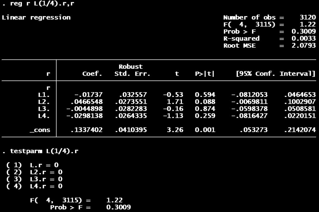
6 Sock reurns are unpredicable

7 Squared Reurns are predicable

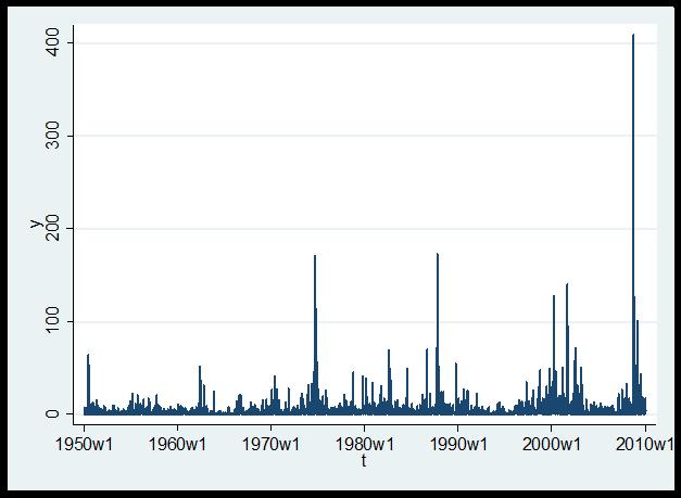
8 Squared Reurns

9 ARCH Rober Engle (198) proposed a model for he condiional variance AuoRegressive Condiional Heeroskedasiciy ARCH now describes volailiy models Nobel Prize 003

10 y σ ARCH(1) Model = ω > α = μ + e var 0 0 ( e Ω ) α>0 means ha he condiional variance is high when he lagged squared error is high Large errors (eiher sign) oday mean high expeced errors (in magniude) omorrow. Small magniude errors forecas nex period small magniude errors. 1 = ω + αe 1

11 Uncondiional variance A propery of expecaions is ha expeced (average) condiional expecaions are uncondiional expecaions. So he average condiional variance is he average variance he variance of he regression error. ( ) ( ) σ = E σ = ω + αe e 1 = ω + ασ Solving for he variance: ω σ = 1 α

12 Rewriing, his implies ω = σ 1 ( α ) Subsiuing ino ARCH(1) equaion ( ) σ = α σ + αe or σ σ + α σ = e ( ) This shows ha he condiional variance is a combinaion of he uncondiional variance, and he deviaion of he squared error from is average value.

13 ARCH(1) as AR(1) in squares The model var ( ) ( ) e Ω E e ω αe 1 implies he regression = Ω = = ω αe 1 e + + u where u is whie noise Thus e squared is an AR(1)

14 .arch r, arch(1) Esimaion

15 Variance Forecas Given he parameer esimaes, he esimaed condiional variance for period is ˆ σ ˆ ˆˆ = ω + αe 1 = ω + α 1 ˆ ˆ ( y ˆ μ) The forecased ou of sample variance is ˆ σ ˆ ( y μ) ˆ n+ 1 = ω + α n ˆ

16 Forecas Inerval for he mean You can use he esimaed condiional sandard deviaion o obain forecas inervals for he mean y Z σ ˆ ˆ n+ 1 n ± α / n+ 1 These forecas inervals will vary in widh depending on he esimaed condiional variance. Wider in periods of high volailiy More narrow in periods of low volailiy

17 ARCH(p) model Allow p lags of squared errors Similar o AR(p) in squares Esimaion: ARCH(8).arch r, arch(1/8) ARCH model wih lags 1 hrough p p e e e e y = + = α α α ω σ μ L

18 .arch r, arch(1/8) ARCH(8) Esimaes

19 ARCH needs many lags Noice ha we included 8 lags, and all appeared significan. This is commonly observed in esimaed ARCH models The condiional variance appears o be a funcion of many lagged pas squares

20 GARCH Model Tim Bollerslev (1986) A suden of Engle Curren faculy a Duke proposed he GARCH model o simplify his problem σ ω + βσ + αe β > ω > α =

21 GARCH(1,1) This makes he variance a funcion of all pas lags: I is also smooher han an ARCH model wih a small number of lags ( ) = + = + + = j j j e e α ω β α βσ ω σ

22 GARCH(p,q) p lags of squared error q lags of condiional variance σ = ω + β σ α e L+ βqσ q + α1e 1 + L+ p p GARCH(1,1):.arch r, arch(1) garch(1) GARCH(3,):.arch r, arch(1/3) garch(1/)

23 GARCH(1,1) Common GARCH feaures Lagged variance has large coefficien Sum of wo coefficiens very close o (bu less han) one

24 GARCH(,) for Sock Reurns

25 GARCH(1,1) The GARCH(1,1) ofen fis well, and is a useful benchmark. Daily, weekly, or monhly asse reurns, exchange raes, or ineres raes

26 Exensions There are many exensions of he basic GARCH model, developed o handle a variey of siuaions Asymmeric Response Garch in mean Explanaory variables in variance Non normal errors

27 Threshold GARCH σ Asymeric GARCH = ω + βσ 1 + αe 1 + γe 11 1 ( e > 0) The las ern is dummy variable for posiive lagged errors This model specifies ha he ARCH effec depends on wheher he error was posiive or negaive If he error is negaive, he effec is α If he error is posiive, he full effec is α+γ

28 TARCH esimaion.arch r, arch(1) arch(1) garch(1) Negaive errors have coefficien of 0.19 Posiive errors have coefficien of 0.05 Negaive reurns increase volailiy much more han posiive reurns

29 Leverage Effec This model describes wha is called he leverage effec A negaive shock o equiy increases he raio deb/equiy of invesors This increases he leverage of heir porfolios This increases risk, and he condiional variance Negaive shocks have sronger effec on variance han posiive shocks

30 GARCH in mean If invesors are risk averse, risky asses will earn higher reurns (a risk premium) in marke equilibrium If asses have varying volailiy (risk), heir expeced reurn will vary wih his volailiy Expeced reurn should be posiively correlaed wih volailiy

31 GARCH M model y σ = β + β σ 1 1 = ω + βσ e + αe 1.arch arch(1) garch(1) archm

32 GARCH M for Sock Reurns Marginally posiive effec

33 TARCH and GARCH M.arch arch(1) arch(1) garch(1) archm archm erm appears insignifican

34 Esimaed sandard deviaion Esimaed TARCH model.predic v, variance.gen s=sqr(v) Uncondiional variance is.1

35 S&P, reurns, and sandard deviaion