Chapter 3: RANDOM VARIABLES and Probability Distributions

Transcription

1 Chapter 3: RANDOM VARIABLES and Probability Distributions 1 RANDOM VARIABLE Definition: A random variable (hereafter rv) X: S R is a numerical valued function defined on a sample space. That is, a number X(a) is assigned to an outcome a in S. Please always keep in mind that a rv X is a function rather than a number, and the value of X depends on an outcome. Throughout this course, we would write the event { X = x } to represent {a S X(a) = x}, the event { X x } to represent {a S X(a) x}, etc. Random variables are often denoted by capital letters, say X, Y, Z, and their possible numerical values (or called realizations) are denoted by the same lowercase letters, say x, y, z. Note that the rv X is a random quantity BEFORE the experiment is performed and its realization x is the value of the random quantity AFTER the experiment has been performed. The word RANDOM reminds us of the fact that we cannot predict the outcomes of the experiment and consequently its associated numerical value beforehand. ~ 1 ~

2 2 PROBABILITY OF A RANDOM VARIABLE To get the probability of a rv itself, we need a function P X ( ) defined below. In other words, the function P X on X(S) for the random variable X is induced by the probability function P on S. QUESTION According to the above definition of the function P X, does P X satisfy the axioms of a probability function? That is, is P X a valid probability function defined on X(S)? Ans: Yes. ~ 2 ~

3 3 PROBABILITY DISTRIBUTION OF A RANDOM VARIABLE Recall that a rv has its own probability law --- a rule that assigns probabilities to the different possible values of the rv (or equivalent, a collection of all values rv can take on along with the probability of each value). Such a probability law or the probability assignment is often called a (probability) distribution. Note that a rv can be fully specified by its distribution. EXAMPLE Suppose we roll a pair of fair/regular hexagonal dice and the rv X represents their sum. This is a tabular form of showing the distribution of a discrete rv. ~ 3 ~

4 Alternatively, a (cumulative) distribution function, denoted by F X (x), can also be used to specify a rv. Definition: A distribution function (or cdf) F X (x) is defined as F X (x) = P X (X x), for all real values x. PROPERTIES We have the following properties of a cdf of a rv: ~ 4 ~

5 Proof: ~ 5 ~

6 Thus, for a < b, This result tells us that P X (X < b) does not necessarily equal F X (b), since F X (b) also includes the probability that X equals b and this probability may not equal zero. Normally, the probabilities for the intervals (a, b), (a, b], [a, b) and [a, b] are not equal, unless the probability at the end point(s) is zero this is always true when the cdf is a continuous function. 4 TWO TYPES OF RANDOM VARIABLES The range of a rv, denoted by χ, is the collection of all possible values it can take on. We then can use χ to classify the rv to be either a Continuous rv, or a Discrete rv. Note that there exists a rv being both discrete and continuous, but we will not discuss this kind of rv in this course. 4.1 DISCRETE RANDOM VARIABLE It is a rv that all of its possible values are isolated points. 4.2 CONTINUOUS RANDOM VARIABLE It is a rv whose range is an interval over the real line. ~ 6 ~

7 5 DISCRETE RANDOM VARIABLE 5.1 PROBABILITY MASS FUNCTION AND DISTRIBUTION FUNCTION (Probability mass function, pmf) The probability MASS function of a DISCRETE rv X, denoted by p X (x), is a function that gives us the probability of occurrence for each possible value x of X. It is valid for all possible values x of X. Conditions for a pmf: o 0 < p X (x) 1, for all x in the range of X. o x χ p X (x) = 1. Cdf of a discrete rv: o F X (a) = P X (X a) = x a p X (x), for all real values a. ~ 7 ~

8 As we have seen, the cdf of a discrete random variable would be a stepfunction with the size p X (a) of the jumps at the possible value a. If the range of the discrete rv X is expressed by {x 1, x 2, x 3, }, then we have p X (x 1 ) = F X (x 1 ) and p X (x j ) = F X (x j ) F X (x j 1 ), where j = 2, 3,. and x 1, x 2, x 3, are sorted in an ascending order. More generally, we have the following result: It can be verified by our previous result that 5.2 POPULATION MEAN AND POPULATION VARIANCE (Population mean) If X is a discrete rv with its pmf p X (x) and its range χ, then the population mean (expectation, expected value) of X is if the sum exists. E(X) = [x p X (x)], x χ The population mean is usually denoted by μ or μ X. It is a common measure of central location of the random variable X. ~ 8 ~

9 (Population variance) If X is a discrete rv with its pmf p X (x) and its range χ, then the population variance of X is if the sum exists. Var(X) = [(x μ) 2 p X (x)], x χ The population variance is usually denoted by σ 2 or σ X 2. The positive square root of σ 2, denoted by σ, is called the population standard deviation (sd) of X. Both of σ 2 and σ are common measures of spread of the random variable X. It can be showed that Var(X) = E(X 2 ) [E(X)] 2. RESULTS Consider a function g of a discrete rv X. We have E[g(X)] = [g(x)p X (x)]. x χ Caution: In general, E[g(X)] g[e(x)]. In particular, if c and d are two constants, then 1. E(cX + d) = ce(x) + d. 2. Var(cX + d) = c 2 Var(X). If there are k constants, say c 1,, c k, and k functions of X, say g 1 (X),, g k (X), then k E [ c i g i (X)] = {c i E[g i (X)]} i=1 ~ 9 ~ k i=1

10 6 DISCRETE DISTRIBUTIONS The following well-known distributions are important in statistics as many results are derived for them leading to quick analyses. In this section, we would study all above discrete distributions. 6.1 BERNOULLI DISTRIBUTION A Bernoulli distribution is related to a random experiment with the following features: A single trial with two possible outcomes denoted by success and failure. The probability of success is p. ~ 10 ~

11 Here are some typical examples for Bernoulli distributions Trial Success Failure (the outcome of our interest) Tossing a coin Head Tail Pure guess in M.C. Correct Wrong Randomly select a product Non-defective Defective If X is the discrete rv of the number of a success in ONE trial, then we can use a Bernoulli distribution to characterize its random behavior. More details about the Bernoulli distribution Notation: X Bernoulli( p) pmf: p X (k) = P X (X = k) = p k (1 p) 1 k, for k = 0, 1; p X (k) = 0, otherwise. Population mean and population variance: E(X) = p, Var(X) = p(1 p). 6.2 BINOMIAL DISTRIBUTION A Binomial distribution is related to a random experiment of repeatedly performing a Bernoulli experiment finite (say, n) times independently. Note that n is a fixed finite number of identical trials, say n <. Trials are independent. Each trial results in two possible outcomes denoted by success and failure. The probability of success p is constant across trials. ~ 11 ~

12 If X is the discrete rv of the number of successes in n trials, then we can use a Binomial distribution to characterize its random behavior. More details about the Binomial distribution Notation: X Binomial(n, p) pmf: p X (k) = P X (X = k) = ( n k ) pk (1 p) n k, for k = 0, 1,, n; p X (k) = 0, otherwise. Population mean and population variance: E(X) = np, Var(X) = np(1 p). Note that the Bernoulli distribution indeed is a special case of a Binomial distribution with n = 1. APPLICATION OF THE BINOMIAL DISTRIBUTION IN FINANCE In investments, the binomial distribution arises in connection with a simplified model for stock prices, which is based on the premise that there is no predictive information in past stock prices, i.e., past prices and price patterns cannot be used to predict future prices and price movements. To see this connection, consider a security whose closing price today is S 0, and let S 1, S 2,, S n be the successive closing prices for this stock over the next n trading days. Suppose that on each day, the piece of the stock either moves up to us previous or down to ds previous, where S previous is the previous day s closing price, and u and d are fixed. ~ 12 ~

13 Graphically, we can use the so-called binomial tree to illustrate this binomial model for stock prices schematically as follows: S 0 u 4 d 0 ud S 0 u 2 d S 0 ud 2 S 0 u 3 d 1 S 0 u 2 d 2 S 0 u 1 d 3 S 0 u 0 d 4 Indeed, the possible values of the stock price S n at time n (or after n days) are in form of S 0 u a d n a, where a is the possible number of times the stock moves up in the n trading days. Suppose further that the probability of an upward movement on each day is p, independent of the stock price movements on the previous days. Correspondingly, if we define X to be a random variable of the number of times the stock moves up in the n trading days. Then, X Binomial(n, p), and the probability that S n = S 0 u a d n a is equivalent to the probability that X = a, where a = 0, 1,, n. ~ 13 ~

14 QUESTION (a) Consider the simplest financial model with a binomial distribution we discuss above. Suppose that the two possible movements of stock price in the model are equally likely. If S 0 = $20, n = 2, u = 2, and d = 1/2, then find i. P(S 2 = $80). ii. P({will get more than the initial stock price}) iii. the expected stock price we can get (b) Show the following general formula of the expected valued of the stock price in the model E(S n ) = S 0 [p(u d) + d] n. ~ 14 ~

15 QUESTION A model for the movement of a stock supposes that, if the present price of the stock is S 0, then after one time period it will either be us 0 with probability p = or ds 0 with probability 1 p. Assuming that successive movements are independent, find the probability that the stock s price will be up at least 7% after nine time periods if u = and d = ~ 15 ~

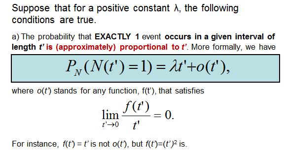
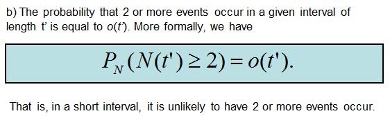
16 6.3 POISSON DISTRIBUTION The next discrete distribution that we will consider is the Poisson distribution. It can be used to determine the probability of counts of the occurrence of an event over time (or space). Here are some typical examples for Poisson distributions. 1. The number of traffic accidents occurring on a highway in a day. 2. The number of people joining a line in an hour. 3. The number of goals scored in a hockey game. 4. The number of typos per page of an essay. More details about the Poisson distribution Notation: X Poisson(λ), where λ (0, ) is the rate of occurrences of an event per unit time (or space) or the average number of occurrences of the event per unit time (or space). pmf: p X (x) = P X (X = x) = λx e λ, for x = 0, 1, ; p X (x) = 0, otherwise. Population mean and population variance: E(X) = λ, Var(X) = λ. x! ~ 16 ~

17 POISSON PROCESS Stochastic (random) process is a collection of random variables often denoted by {N(t), t Λ}. If Λ contains isolated points like {0, 1, 2,, }, then the process is called a discrete-time process, while if Λ is an interval like [0, ), then the process is called a continuous-time process. Here are examples of the stochastic process: N(t) for each t Λ Discrete Continuous Discrete Random walk Poisson process Continuous Time-series Brownian motion Stock market fluctuations can be modeled by stochastic processes (like random walk). In this section, we focus on the Poisson process --- the stochastic process with Λ = [0, ). In Poisson process, N(t) represents a number of occurrences of an event/accident within time interval [0,t], where N(0) = 0. Under certain conditions, we can prove that N(t) follows a Poisson distribution. ~ 17 ~

18 ~ 18 ~ MATH2421: Probability Dr. YU, Chi Wai

19 Proof: Discussed in lecture. QUESTION Consider a number of telephone calls received by an office in an hour. Now assume that the average phone call per hour is 3 and the number of phone call per hour has a Poisson distribution. Find a) P(2 phone calls in 30 minutes), and b) P(less than 8 phone calls in 2 hours) POISSON APPROXIMATION TO BINOMIAL PROBABILITY Here we observe that an infinity-outcome experiment can be regarded as a limit of a noutcome experiment as n goes to infinity. So, it is natural to ask if the limit of a Binomial probability is a Poisson probability. Question: Is the limit of a Binomial probability a Poisson probability? If yes, then which Poisson probability is the limit of a Binomial (n, p) probability? Ans: Yes, and note that ( n x ) px (1 p) n x (np)x e (np) 0 as n x! ~ 19 ~

20 Therefore, if n is large and p is small enough so that np <, then we can use Poisson (np) to approximate the probability of X ~ Binomial(n, p). Roughly speaking, the Poisson approximation is good if n 20 and p 0. 05, and is excellent when n 100 and np < 10. QUESTION A computer hardware company manufacturers a particular type of microchip. There is a 0.1% chance that any given microchip of this type is defective, independent of the other microchips produced. Determine the probability that there are at least two defective microchips in a shipment of exactly, and 2. approximately by a Poisson distribution. RELATIONSHIP WITH OTHER DISTRIBUTION: We have just discussed that a Poisson distribution can be regarded as the limiting distribution of Binomial. Indeed, a Poisson distribution also relates to an EXPONENTIAL and GAMMA distributions, where both of them are distributions for continuous random variables. We will come back to discuss their relationships in next section. For the sake of completeness, let us have a look at the relationship here: ~ 20 ~

21 6.4 NEGATIVE BINOMIAL DISTRIBUTION Recall that for a Binomial distribution, the number of trials is fixed and the number of getting a success outcome is random. So, if we reverse them, i.e. we consider the random number of trials required to get a fixed number (say, k 1) of success outcomes, then what distribution can we use to describe the randomness of this random variable? Negative Binomial distribution is the distribution that we can use for the random number of trials required to get k success. More details about the Negative Binomial distribution Notation: pmf: X N. Bin(k, p), where 0 < p < 1 p X (n) = P X (X = n) = ( n 1 k 1 ) (1 p)n k p k, n = k, k + 1, ; p X (n) = 0, otherwise. Population mean and population variance: REMARK: E(X) = k p, Var(X) = k(1 p) p 2. Similar to a Binomial distribution, Negative Binomial distribution also requires (1) each trial results in two possible outcomes denoted by success and failure, and (2)The probability of success p is constant across trials. P X (X s) can be interpreted as a probability of getting k success before s-k+1 failures, if X N. Bin(k, p). ~ 21 ~

22 If k = 1, then the negative binomial distribution will reduce to the so-called Geometric distribution --- the distribution of the random number X of trials required until a success/the first success occurs. Notationally, we have X ~Geometric(p). o The geometric distribution is the unique positive discrete distribution which enjoys the memoryless property: That is, for any positive integers s and t, P X (X > s + t X > t) = P X (X > s). ~ 22 ~

23 QUESTION A box contains N white and M black balls. Balls are randomly selected, one at a time, until a black one is obtained. If we assume that each selected ball is put back to the box before the next one is drawn, what is the probability that a) Exactly n draws are needed; b) At least k draws are needed. QUESTION A comedian tells jokes that are only funny 25% of the time. What is the probability that he tells his tenth funny joke in his fortieth attempt? ~ 23 ~

24 QUESTION In successive rolls of a pair of fair dice, what is the probability of getting 2 (sums of) 7 s before 6 (sums of) even numbers? The answer can be obtained by using a negative binomial distribution. HOW? Note that the desired probability looks very similar to the above-mentioned interpretation of P X (X s) with k = 2 and s k + 1 = 6 (s = 7). So, we can set P X (X 7) to be the desired probability. Therefore, the probability can be found by 7 P X (X 7) = ( n 1 1 ) (1 p)n 2 p 2, where X N. Bin(2, p). n=2 What is p? Is p = P("7") correct? According to the above setting, we cannot simply let 7 and even numbers be success and failure, respectively, to say p = P("7"). This is so because 7 and even numbers are not valid success and failure outcomes --- success and ~ 24 ~

25 failure must be disjoint and exhaustive, but 7 and even numbers are disjoint only and they are NOT exhaustive. Therefore, p P("7"). Then, what is p?... 7 and even numbers cannot be valid success and failure because they are NOT exhaustive. Thus, we may ask ourselves the following natural question Is it possible to make 7 and even become valid success and failure? Or equivalently, can we make them be exhaustive? One possible way to get Yes is to consider a collection Ω of getting 7 or even only. In Ω, 7 and even are disjoint and exhaustive! We thus can define X in Ω and get p = P("7" Ω ) = P("7") P(Ω ) = P("7") P(7) + P("even") = Based on this heuristic value of p, we have the result that P X (X 7) = ( n 1 1 ) (1 p)n 2 p 2 = n=2 = 1 4 ~ 25 ~

26 Is p = P("7" Ω ) correct? To answer this question, we need to modify the original question a little bit: In successive rolls of pair of fair dice, what is the probability of getting a (sum of) 7 before an (sum of) even number? If negative binomial distribution is used to find the above probability, then we can consider X N. Bin(1, p) and the above probability can be set to be P X (X 1). Note that in this case P X (X 1) = P X (X = 1) = p. That is, the true meaning of p indeed is the probability of getting a 7 before an even number. Okay. Then, is the probability of getting a 7 before an even number equal to P("7" Ω )? The answer is Yes. The following is the proof. Proof: First consider the possible outcome on the 1 st trial. Let A be the event that 7 occurs, B be the event that even occurs, and C be the event that other ~ 26 ~

27 occurs. Note that A, B and C are mutually exclusive and exhaustive. Then, by the law of total probability, we have P(a 7 before an even ) = P(a 7 before an even A) P(A) + P(a 7 before an even B) P(B) + P(a 7 before an even C) P(C) where P(A) = 1, P(B) = 1, P(C) = 1 P(A) P(B). 6 2 For the three conditional probabilities, we observe that if A occurs, then the event {a 7 before an even } occurs certainly, so P(a 7 before an even A) = 1. if B occurs, then the event {a 7 before an even } does NOT occur certainly, so P(a 7 before an even A) = 0. if C occurs, then we have no relevant information to determine whether 7 or even occurs first. Thus, we need to start all over again, and then get P( 7 before even C) = P( 7 before even ). In other words, P(a 7 before an even ) = P(A) + P(a 7 before an even ) [1 P(A) P(B)] That is, P(a 7 before an even ) = where Ω = {"7", "even"}. P(A) P(A)+P(B) = P("7") P("7" or "even" ) = P("7" Ω ), More generally, we have the following result: Suppose that E and F are disjoint events of an experiment. If independent trials of this experiment are performed, then E will occur before F with probability P(E) P(E) + P(F) Note that if E and F are also exhaustive, then the probability would reduce to the usual probability P(E) that E occurs. ~ 27 ~

28 Challenging question for students: Prove that if X N. Bin(k, p) and Y Binomial(s, p), then P X (X s) = P Y (Y k). Hint: Let A = {get k success before s k + 1 failures} and consider A c with a binomial distribution. 6.5 HYPERGEOMETRIC DISTRIBUTION Recall that one of the conditions for a Binomial distribution is the constant p across all n trials. If this condition is violated (this is equivalent to saying that the trials are not independent), then we can use Hypergeometric distribution to describe the randomness of the number of success outcomes. Typical Example: Consider a box of N balls, where m balls are white and N m balls are black. Now, take n balls out without replacement, and X is the number of white balls in the sample of n balls. More details about the Hypergeometric distribution Notation: X Hypergeo(n, m, N), pmf: p X (k) = (m k )(N m n k ) ( N n ), for max(0, n + m N) k min (m, n); p X (k) = 0, otherwise. Population mean and population variance: E(X) = nm N, Var(X) = N n N 1 np(1 p) with p = m N. ~ 28 ~

29 RELATIONSHIP BETWEEN BINOMIAL AND HYPERGEOMETRIC DISTRIBUTIONS If m and N are large in relation to n, then the Hypergeometric distribution can be approximated by the Binomial distribution. QUESTION A lot of 1000 items consist of 100 defective and 900 good items. A sample of 20 items is randomly taken without replacement. Find the probability that the sample contains two or less defective items. ~ 29 ~

30 7 A DISTRIBUTION OF A REAL-VALUED FUNCTION OF A DISCRETE RV There are many problems in which we are interested not only in the expected value of a rv X, but also in the expected values of rv related to X. To be more precise, we might be interested in the expectation of the rv Y, whose values y are related to the values x of X by means of the equation y = g(x). Correspondingly, we have Y = g(x). Recall that we have already seen the result before that E[g(X)] = [g(x)p X (x)]. x χ Now it is a time to see why we have such a result. First, we need determine the probability distribution or the pmf of Y = g(x). Note that if x 1, x 2, are the possible values of X, then g(x 1 ), g(x 2 ), are the possible values of Y, and Y is also a discrete rv. Here we can see that some of g(x i ) may be equal to each other. For instance, suppose g(x 1 ) = g(x 5 ) = y 1 and g(x j ) y 1 for other j 1 or 5. Then, p Y (y 1 ) = P Y (Y = y 1 ) = P X ({X = x 1 } {X = x 5 }) = P X (X = x 1 ) + P X (X = x 5 ) In other words, the pmf of Y can be found by using the above method to determine the probability of each of its possible values. ~ 30 ~

31 More generally, define χ Y = {y = g(x), x χ X }, and for each y χ Y, we can define a subset of χ X by χ y = {x χ X g(x) = y}. Consequently, we have the results and for each y χ Y, χ X = χ y y χ Y p Y (y) = p X (x) x χ y. So, E[g(X)] = E(Y) = [yp Y (y)] = [y p X (x) y χ Y y χ Y x χ y ] = [g(x)p X (x)] y χ Y x χ y = [g(x)p X (x)] x χ X. ~ 31 ~

32 The following example is provided to illustrate the above idea how to determine the pmf of a function of a discrete r.v. X. EXAMPLE Consider a discrete rv X whose range is χ X = {0, 1,2, 3, 4, 5}, and Y = (X 2) 2. Thus, the range of Y is χ Y = {0, 1, 4, 9} For each possible value of Y in χ Y, we can get a collection of some particular elements in χ X. To be more precise, we have χ 0 = {2}, χ 1 = {1,3}, χ 4 = {0,4}, χ 9 = {5} Note that the subscribes are the values in χ Y, and the collections are mutually exclusive and their union is χ X. Thus, we can use one of the above collections to get the probability of a particular value of Y in χ Y. For instance, p Y (1) = p X (x) x χ 1 = p X (1) + p X (3) p Y (9) = p X (x) x χ 9 = p X (5) The pmf or distribution of Y = g(x) y p Y (y) ~ 32 ~

33 8 CONTINUOUS RANDOM VARIABLE 8.1 PROBABILITY DENSITY FUNCTION AND DISTRIBUTION FUNCTION (Probability density function, pdf) The probability DENSITY function of a CONTINUOUS rv X, denoted by f X (x), is a function that gives us a value for the measure of how likely it is that X is near to x. It is valid for all possible values x of X. Conditions for a pdf: o 0 < f X (x), for all x in the range of X. o f X (x) dx = 1. Note that the value of f X (x) does NOT give us the probability that the corresponding random variable takes on the value x. Indeed, in the continuous case, the probabilities are given by integrating f X (x) over a particular interval in the following way. Probability that X belongs to A: Cdf of a continuous rv: P X (X A) = f X (x) dx. x A o F X (a) = P X (X a) = a f X (x) dx, for all real values a. Convert F X (a) to f X (a): f X (a) = d da F X(a). ~ 33 ~

34 To be more precise, F X (a + δa) F X (a) P X (a < X a + δa) f X (a) = lim = lim. δa 0 δa δa 0 δa Thus, if the length of the interval (a, a + δa] is small enough, then P X (a < X a + δa) f X (a)δa. Therefore, we can interpret f X (a) as a measure of how likely it is that X will be near the point a. Recall that if F X is continuous, then for any real b, P X (X < b) = lim n F X (b 1 n ) = F X [ lim n (b 1 n )] = F X(b) = P X (X b), which implies P X (X = b) = 0. Thus, for any continuous r.v. X, when a < b, we have P X (a < X < b) = P X (a X b) = P X (a X < b) = P X (a < X b) = F X (b) F X (a). 8.2 POPULATION MEAN AND POPULATION VARIANCE (Population mean) If X is a continuous rv with its pdf f X (x), then the population mean (expectation, expected value) of X is defined as E(X) = [x f X (x)] dx, if it exists. The population mean is usually denoted by μ or μ X. It is a common measure of central location of the random variable X. ~ 34 ~

35 (Population variance) If X is a continuous rv with its pdf f X (x), then the population variance of X is defined as Var(X) = [(x μ) 2 f X (x)] dx, if it exists. The population variance is usually denoted by σ 2 or σ X 2. The positive square root of σ 2, denoted by σ, is called the population standard deviation (sd) of X. Both of σ 2 and σ are common measures of spread of the random variable X. It can be showed that Var(X) = E(X 2 ) [E(X)] 2. RESULTS Consider a function g of a continuous rv X. We have E[g(X)] = [g(x)f X (x)] dx Caution: In general, E[g(X)] g[e(x)]. In particular, if c and d are two constants, then 1. E(cX + d) = ce(x) + d. 2. Var(cX + d) = c 2 Var(X). If there are k constants, say c 1,, c k, and k functions of X, say g 1 (X),, g k (X), then k E [ c i g i (X)] = {c i E[g i (X)]} i=1 ~ 35 ~ k i=1

36 9 CONTINUOUS DISTRIBUTIONS In the following, we would study several important continuous distributions. 9.1 NORMAL DISTRIBUTION The most important continuous probability distribution in the field of statistics and probability is the Normal distribution because it accurately describes many practical and significant real-world quantities such as noise, voltage, current, electrons, and other quantities which are results from many small independent random terms. It is sometimes called the Gaussian distribution because it was given by Johann Carl Friedrich Gauss --- the Prince of Mathematics. ~ 36 ~

37 Johann Carl Friedrich Gauss (30 April February 1855) was a German mathematician whose contributions included too many fields, such as number theory, algebra, statistics, analysis, differential geometry, geophysics, mechanics, mechanics, electrostatics, astronomy and optics. From 1989 through 2001, Gauss's portrait and a normal density curve were featured on the German ten-mark banknote. More about Gauss can be found on More details about the Normal distribution Notation: X N(a, b), where a (, ) and b (0, ). pdf: f(x) = 1 2πb e 1 2b (x a)2, for all real values x. Population mean and population variance: E(X) = a, Var(X) = b. ~ 37 ~

38 Because of the last results, most people like using the following notation and pdf for the normal distribution. Notation: X N(μ, σ 2 ), where μ (, ) and σ (0, ). pdf: f(x) = 1 1 e2σ 2(x μ)2, for all real values x. 2πσ2 Note that all normal distributions have bell-shaped density curves regardless of the values of and. Under any normal density curve, we can also find that there are around 0.68 (or 0.95 or 0.99) probability that the rv X is within 1 (or 2 or 3) sd from its population mean. ~ 38 ~

39 STANDARD NORMAL DISTRIBUTION Through the standard normal distribution --- the simplest normal distribution with mean 0 and variance 1, i.e. N(0, 1), we can show that areas under all normal curves are related with one another. Indeed, we can find an area over an interval for any normal curve by just finding the corresponding area under a standard normal density curve. The random variable following the standard normal distribution is often denoted by Z in probability and statistics, and the cdf of the standard normal distribution is denoted by Φ(a), instead of P Z (Z a). By the symmetry of a standard normal density curve, we can show that for any real a, Φ(a) = 1 Φ( a). ~ 39 ~

40 STANDARDIZATION Standardization is a process used to transform any normal-distributed r.v., say X ~ N(μ, σ 2 ), to a standard normal-distributed r.v. Z ~ N(0, 1). To be more precise, we have the following result: If X ~ N(μ, σ 2 ), and then we standardize X, i.e. subtract μ from X and then divide by σ then X μ σ Thus, notationally, we have Z = X μ ~ N(0, 1). σ, or X = μ + σz. Conversely, if Z ~ N(0, 1), then μ + σz N(μ, σ 2 ). We will come back to prove this result in section 10. According to the standardization, the probability of any normal-distributed r.v. can be reduced to the probability of a standard normal-distributed r.v. In other words, if we want to find a probability of X, it suffices for us to know how to find the probability of Z. ~ 40 ~

41 STANDARD NORMAL TABLE The standard normal table provided on the course webpage gives the area under the standard normal curve corresponding to P( Z z) for the values of z ranging from 3.89 to More precisely, we would have a table below ~ 41 ~

42 NORMAL APPROXIMATION TO THE PROBABILITY OF AN INTEGER-VALUED DISCRETE R.V. Normal distribution is important partly because we can use it to approximate any distribution. In particular, when we use it (a continuous distribution) to approximate an integer-valued discrete distribution ---- the possible values of the corresponding discrete r.v. are integers with 1 unit of step sizes, we need to make an adjustment (often called continuity correction) so as to get a better approximation. Continuity correction: If X is an integer-valued discrete random variable with mean μ X and variance σ X 2, then we use N(μ X, σ X 2 ) with an adjustment ±0. 5 to approximate the probability of X. In term of Z or a standard normal distribution, we finally have ~ 42 ~

43 For instance, 1. The Normal approximation to a Binomial probability P X (X = k), if X Binomial(n, p) is given by P Z (Z k np np(1 p) ) P k 0.5 np Z (Z np(1 p) ). 2. The Normal approximation to a Poisson probability P X (X = k), if X Poisson(λ) is given by P Z (Z k λ ) P Z (Z λ k 0.5 λ ). λ Roughly speaking, the normal approximation to Binomial is good when min{np, n(1 p)} 10, and to Poisson is good when λ 20. ~ 43 ~

44 EXAMPLE It is believed that 4% of children have a gene that may be linked to teenage diabetes. Researchers are hoping to track 20 or more of these children (with the defect) for several years. They will test 732 newborn babies for the presence of this gene, and if the gene is present, they will track the child for several years. Find the normal approximated probability that they would find 20 or more subjects to be in the study. Answer: Let X be the random variable of the number of eligible children. So, X Binomial(n = 732, p = 0.04). Using Normal distribution N(np = 29.28, np(1 p) = 28.1) to approximate to the Binomial probability, we have P X (X 20) P Z (Z ) 28.1 = P Z (Z 1.85) = , where the exact Binomial probability is ~ 44 ~

45 QUESTION (1) Given a coin such that P({head}) = 1/3. Toss it 100 times. What is the normal approximated probability that head shows up 30 or more times? (2) Consider the number of large earthquakes in California. Assume that the random variable of this number has a Poisson distribution with a rate of 1.5 per year. Find the normal approximated probability of having more than 14 large earthquakes in the next 15 years. ~ 45 ~

46 9.2 GAMMA DISTRIBUTION It is one of the distributions of non-negative continuous rv X, i.e. the range of X contains all non-negative real values. In practice, a Gamma distribution often arises as being the distribution of the amount of time until a certain number of a specific event (say, an accident) occurs. For instance, the time until 5 earthquakes occur, the time until 10 telephone calls we receive turn out to be a wrong number, and so on, are all random variables that tend in practice to follow Gamma distributions. In addition, it is also a commonly used distribution in survival analysis for the lifetime of a subject, and in genomics, it is often applied in recognition in ChIP-seq analysis --- a new approach for genomewide mapping of protein binding sites on DNA. A random variable X is said to follow a Gamma distribution with parameters α and β, denoted by Gamma(α, β),where α (0, ) and β (0, ), if its pdf can be written as f X (x) = { β α Γ(α) xα 1 e βx, if x 0; where Γ(t), called a gamma function, is defined as PROPERTIES OF Γ(t): 0, if x < 0, Γ(t) = (x t 1 e x ) dx. For any positive real value t, Γ(t) = (t 1)Γ(t 1). For any positive integer n, Γ(n) = (n 1)!. Γ ( 1 2 ) = π. 0 ~ 46 ~

47 REMARKS: If X Gamma(α, β), then E(X) = α β and Var(X) = α β 2. If θ is a positive integer, then Gamma ( θ, 1 ) is the chi-squared distribution 2 2 with θ degrees of freedom. If α = 1, then the Gamma distribution reduces to an EXPONENTIAL distribution with a parameter β, denoted by Exp(β). o In general, there is no simple form of the cdf of a Gamma distribution, except α = 1. In other words, we have a simple form of the cdf of Exp(β): 1 e βa, if a > 0; F X (a) = { 0, if a 0, o An exponential distribution is the unique non-negative continuous distribution to have an memoryless property: That is, for any positive s and t, P X (X > s + t X > t) = P X (X > s) or equivalently, P X (X > s + t) = P X (X > s)p X (X > t) ~ 47 ~

48 ~ 48 ~ MATH2421: Probability Dr. YU, Chi Wai

49 EXAMPLE Suppose that the lifetime of the battery of a cell phone is exponentially distributed with an average value of 5 hours. If a person desires to make a call for three hours, what is the probability that he/she will be able to compute the call without having to replace the battery? Answer: Let X denote the lifetime of the battery. Then, X Exp(1/5). Now, let t be the number of hours the battery had been in use prior to the start of the phone call. Thus, the desired probability is P X (X > t + 3 X > t) = P X (X > 3) = 1 F X (3) = 1 [1 e 1 5 (3) ] = e RELATIONSHIP WITH A POISSON PROCESS When we studied a Poisson Process, we mentioned before that To be more precise, for any finite t 0, P Y (Y t) = P N (N(t) α), where Y Gamma(α, λ) with a positive integer α, and N(t) Poisson(λt) with λ (0, ). ~ 49 ~

50 Now, let us discuss more details of this relationship ~ 50 ~

51 9.3 BETA DISTRIBUTION A Beta distribution is a continuous distribution often used to fit solar irradiation data from weather stations around the world, and to indicate the condition of a gear in applied acoustics --- a scientific study of sound and sound waves. Correspondingly, a random variable X is said to follow a Beta distribution with parameters a and b, denoted by Beta(a, b),where a (0, ) and b (0, ), if its pdf can be written as f X (x) = x a 1 (1 x) b 1, if x (0,1); B(a, b) { 0, otherwise, where B(a, b), called a beta function, is defined as 1 B(a, b) = [x a 1 (1 x) b 1 ] dx. 0 PROPERTIES OF B(a, b): B(a, b) = a+b = B(a, b) = Γ(a)Γ(b) Γ(a+b). a a+b B(a + 1, b) = b B(a, b + 1) (a + b)(a + b + 1) B(a + 1, b + 1). ab ~ 51 ~

52 REMARKS: If X Beta(a, b), then E(X) = a a+b and Var(X) = ab (a+b) 2 (a+b+1). If a = b = 1, then the Beta distribution reduces to a UNIFORM distribution over an interval (0, 1), denoted by U (0,1). o More generally, a UNIFORM distribution can be defined on an interval (k 1, k 2 ], [k 1, k 2 ], (k 1, k 2 ), or [k 1, k 2 ), where k 1 < k 2 with its pdf given by 1, if x (k k f X (x) = { 2 k 1, k 2 ], [k 1, k 2 ], (k 1, k 2 ), or [k 1, k 2 ); 1 0, otherwise, o Note that the pdf of a uniform distribution is always a constant over the interval. o A uniform distribution often arises in the study of rounding errors when measurements are recorded to certain accuracy. For instance, if measurements of daily temperatures are recorded to the nearest degree, it would be assumed that the difference in degrees between the true and the recorded temperatures is within a particular interval, say between -0.5 and 0.5 equally, and then the error can be said to follow a uniform distribution over this interval. ~ 52 ~

53 QUESTION Buses arrive at a specified stop at 15-minute intervals starting at 7am. That is, they arrive at 7, 7:15, 7:30, and so on. If you arrive at the stop at a time that is uniformly distributed between 7am and 7:30am, then find the probability that you have to wait (a) less than 5 minutes for a bus, and (b) more than 10 minutes for a bus. ~ 53 ~

54 10 A DISTRIBUTION OF A REAL-VALUED FUNCTION OF A CONTINUOUS RV Consider a continuous rv X with its pdf f X and cdf F X. If now we have a continuous function g and define Y = g(x), then we can use the following approach to determine the distribution or pdf of Y: (i) Find the cdf of Y, i.e. F Y (y) for any real y, in terms of F X. (ii) Then, find the pdf of Y by in terms of pdf f X. f Y (y) = d dy F Y(y) Using this technique, we can find more relationship among distributions, like the question below. ~ 54 ~

55 QUESTION Show that if X N(0, 1), then X 2 follows a chi-squared distribution with 1 degree of freedom. ~ 55 ~

56 If g is a strictly monotonic (i.e. either increasing or decreasing) and differentiable function, then we would have the following result to find the pdf of Y = g(x) directly: Note that g 1 (y) is defined to be the value of x such that g(x) = y. ~ 56 ~

57 QUESTION Continue the proof by showing the result for any decreasing and differentiable function g. PROOF FOR STANDARDIZATION Recall that if X ~ N(μ, σ 2 ), then X μ N(0, 1), and conversely, if σ Z ~ N(0, 1), then μ + σz N(μ, σ 2 ). Now it is a time for us to see how to get these results. ~ 57 ~

58 LOG-NORMAL DISTRIBUTION In addition to using a Gamma distribution to model a positive-valued random variable, we can also use a LOG-NORMAL distribution. In practice, log-normal distributions are often used for modelling stock pricing, wind speed, and so on. To be more precise, a random variable X is said to be log-normally distributed with parameters μ and σ 2 if its (natural) logarithm follows N(μ, σ 2 ). That is, lnx N(μ, σ 2 ), or equivalently, X = e Y, where Y N(μ, σ 2 ). ~ 58 ~

59 Note that the moment generating function of a log-normal distribution does not exist, so we need to use the standard way to get its population mean and variance. ~ 59 ~

60 Using similar technique, we can show that Var(X) = e 2μ+σ2 (e σ2 1). ~ 60 ~

61 APPLICATION OF LOG-NORMAL DISTRIBUTION IN A FINANCIAL PROBLEM Let S n be the r.v. of the price of an asset (or security or stock) at time n. If the log return, r n = ln ( S n S n 1 ), of the asset has a normal distribution with mean E(r n ) = , and variance Var(r n ) = (0.0663) 2, then what are the mean and standard deviation of the simple return R n = S n S n 1 S n 1? ~ 61 ~

62 Challenging question for students: Show that if X is a continuous rv with its cdf F X, then show that F X (X) U [0,1]. This result tells us that if a continuous rv U U [0,1], then X and F X 1 (U) would have the same distribution. Here is the proof of the result on E(g(X)) in continuous cases. ~ 62 ~