Machine Learning Chapter 4. Algorithms

Size: px

Start display at page:

Download "Machine Learning Chapter 4. Algorithms"

Jason Richardson
6 years ago
Views:

1 Machine Learning Chapter 4. Algorithms

2 4 Algorithms: The basic methods Simplicity first: 1R Use all attributes: Naïve Bayes Decision trees: ID3 Covering algorithms: decision rules: PRISM Association rules Linear models Instance-based learning 2

3 Simplicity first Simple algorithms often work very well! There are many kinds of simple structure, eg: One attribute does all the work All attributes contribute equally & independently A weighted linear combination might do Instance-based: use a few prototypes Use simple logical rules Success of method depends on the domain 3

4 Inferring rudimentary rules 1R: learns a 1-level decision tree I.e., rules that all test one particular attribute Basic version One branch for each value Each branch assigns most frequent class Error rate: proportion of instances that don t belong to the majority class of their corresponding branch Choose attribute with lowest error rate (assumes nominal attributes) 4

5 Pseudo-code for 1R For each attribute, For each value of the attribute, make a rule as follows: count how often each class appears find the most frequent class make the rule assign that class to this attribute-value Calculate the error rate of the rules Choose the rules with the smallest error rate Note: missing is treated as a separate attribute value 5

6 Evaluating the weather attributes Outlook Temp Humidity Windy Play Sunny Hot High False No Sunny Hot High True No Overcast Hot High False Yes Rainy Mild High False Yes Rainy Cool Normal False Yes Rainy Cool Normal True No Overcast Cool Normal True Yes Sunny Mild High False No Sunny Cool Normal False Yes Rainy Mild Normal False Yes Sunny Mild Normal True Yes Overcast Mild High True Yes Overcast Hot Normal False Yes Rainy Mild High True No Attribute Rules Errors Total errors Outlook Sunny No 2/5 4/14 Overcast Yes 0/4 Rainy Yes 2/5 Temp Hot No* 2/4 5/14 Mild Yes 2/6 Cool Yes 1/4 Humidity High No 3/7 4/14 Normal Yes 1/7 Windy False Yes 2/8 5/14 True No* 3/6 * indicates a tie 6

7 Dealing with numeric attributes Discretize numeric attributes Divide each attribute s range into intervals Sort instances according to attribute s values Place breakpoints where the class changes (the majority class) This minimizes the total error Example: temperature from weather data Yes No Yes Yes Yes No No Yes Yes Yes No Yes Yes No 7

8 Dealing with numeric attributes Discretize numeric attributes Divide each attribute s range into intervals Sort instances according to attribute s values Place breakpoints where the class changes (the majority class) This minimizes the total error Outlook Temperature Humidity Windy Play Sunny False No Example: temperature from weather data Sunny True No Overcast False Yes Rainy False Yes Yes No Yes Yes Yes No No Yes Yes Yes No Yes Yes No 8

9 The problem of overfitting This procedure is very sensitive to noise One instance with an incorrect class label will probably produce a separate interval Also: time stamp attribute will have zero errors Simple solution: enforce minimum number of instances in majority class per interval Example (with min = 3): Yes No Yes Yes Yes No No Yes Yes Yes No Yes Yes No Yes No Yes Yes Yes No No Yes Yes Yes No Yes Yes No9

10 With overfitting avoidance Resulting rule set: Attribute Rules Errors Total errors Outlook Sunny No 2/5 4/14 Overcast Yes 0/4 Rainy Yes 2/5 Temperature 77.5 Yes 3/10 5/14 > 77.5 No* 2/4 Humidity 82.5 Yes 1/7 3/14 > 82.5 and 95.5 No 2/6 > 95.5 Yes 0/1 Windy False Yes 2/8 5/14 True No* 3/6 10

Discussion of 1R 1R was described in a paper by Holte (1993) Contains an experimental evaluation on 16 datasets (using cross-validation so that results were representative of performance on future

11 Discussion of 1R 1R was described in a paper by Holte (1993) Contains an experimental evaluation on 16 datasets (using cross-validation so that results were representative of performance on future data) Minimum number of instances was set to 6 after some experimentation 1R s simple rules performed not much worse than much more complex decision trees Simplicity first pays off! Very Simple Classification Rules Perform Well on Most Commonly Used Datasets Robert C. Holte, Computer Science Department, University of Ottawa 11

12 Discussion of 1R: Hyperpipes Another simple technique: build one rule for each class Each rule is a conjunction of tests, one for each attribute For numeric attributes: test checks whether instance s value is inside an interval Interval given by minimum and maximum observed in training data For nominal attributes: test checks whether value is one of a subset of attribute values Subset given by all possible values observed in training data Class with most matching tests is predicted 12

13 Statistical modeling Opposite of 1R: use all the attributes Two assumptions: Attributes are equally important statistically independent (given the class value) I.e., knowing the value of one attribute says nothing about the value of another (if the class is known) Independence assumption is never correct! But this scheme works well in practice 13

14 Probabilities for weather data Outlook Temperature Humidity Windy Play Yes No Yes No Yes No Yes No Yes No Sunny 2 3 Hot 2 2 High 3 4 False Overcast 4 0 Mild 4 2 Normal 6 1 True 3 3 Rainy 3 2 Cool 3 1 Sunny 2/9 3/5 Hot 2/9 2/5 High 3/9 4/5 False 6/9 2/5 9/14 5/14 Overcast 4/9 0/5 Mild 4/9 2/5 Normal 6/9 1/5 True 3/9 3/5 Rainy 3/9 2/5 Cool 3/9 1/5 14

15 Probabilities for weather data Outlook Temperature Humidity Windy Play Yes No Yes No Yes No Yes No Yes No Sunny 2 3 Hot 2 2 High 3 4 False Overcast 4 0 Mild 4 2 Normal 6 1 True 3 3 Rainy 3 2 Cool 3 1 Sunny 2/9 3/5 Hot 2/9 2/5 High 3/9 4/5 False 6/9 2/5 9/14 5/14 Overcast 4/9 0/5 Mild 4/9 2/5 Normal 6/9 1/5 True 3/9 3/5 Rainy 3/9 2/5 Cool 3/9 1/5 Outlook Temp Humidity Windy Play Sunny Hot High False No Sunny Hot High True No Overcast Hot High False Yes Rainy Mild High False Yes Rainy Cool Normal False Yes Rainy Cool Normal True No Overcast Cool Normal True Yes Sunny Mild High False No Sunny Cool Normal False Yes Rainy Mild Normal False Yes Sunny Mild Normal True Yes Overcast Mild High True Yes Overcast Hot Normal False Yes Rainy Mild High True No 15

16 Probabilities for weather data Outlook Temperature Humidity Windy Play Yes No Yes No Yes No Yes No Yes No Sunny 2 3 Hot 2 2 High 3 4 False Overcast 4 0 Mild 4 2 Normal 6 1 True 3 3 Rainy 3 2 Cool 3 1 Sunny 2/9 3/5 Hot 2/9 2/5 High 3/9 4/5 False 6/9 2/5 9/14 5/14 Overcast 4/9 0/5 Mild 4/9 2/5 Normal 6/9 1/5 True 3/9 3/5 Rainy 3/9 2/5 Cool 3/9 1/5 A new day: Outlook Temp. Humidity Windy Play Sunny Cool High True? Likelihood of the two classes For yes = 2/9 3/9 3/9 3/9 9/14 = For no = 3/5 1/5 4/5 3/5 5/14 = Conversion into a probability by normalization: P( yes ) = / ( ) = P( no ) = / ( ) =

Bayes s rule Probability of event H given evidence E : Pr[ H E] Pr[ E H ]Pr[ H ] Pr[ E] A priori probability of H : Probability of event before evidence is seen Pr[ H E] A

17 Bayes s rule Probability of event H given evidence E : Pr[ H E] Pr[ E H ]Pr[ H ] Pr[ E] A priori probability of H : Probability of event before evidence is seen Pr[ H E] A posteriori probability of H : Pr[H ] Probability of event after evidence is seen Thomas Bayes Born: 1702 in London, England Died: 1761 in Tunbridge Wells, Kent, England 17

18 Naïve Bayes for classification Classification learning: what s the probability of the class given an instance? Evidence E = instance Event H = class value for instance Naïve assumption: evidence splits into parts (i.e. attributes) that are independent Pr[H E] Pr[E H]Pr[E H]Pr[E H]Pr[H] 1 2 n Pr[E] 18

19 Weather data example Outlook Temp. Humidity Windy Play Sunny Cool High True? Evidence E Pr[ yes E] Pr[ Outlook Sunny yes] Pr[ Temperature Cool yes] Probability of class yes Pr[ Humidity High Pr[ Windy True Pr[ yes] Pr[ E] yes] yes] Pr[ E]

20 The zero-frequency problem What if an attribute value doesn t occur with every class value? (e.g. Humidity = high for class yes ) Probability will be zero! Pr[ Humidity High yes] 0 A posteriori probability will also be zero! Pr[ yes E] 0 (No matter how likely the other values are!) Remedy: add 1 to the count for every attribute value-class combination (Laplace estimator) Result: probabilities will never be zero! (also: stabilizes probability estimates) 20

21 Modified probability estimates In some cases adding a constant different from 1 might be more appropriate Example: attribute outlook for class yes 2 / / / 3 9 Sunny Overcast Rainy Weights don t need to be equal (but they must sum to 1) p p p

22 Missing values Training: instance is not included in frequency count for attribute valueclass combination Classification: attribute will be omitted from calculation Example: Outlook Temp. Humidity Windy Play? Cool High True? Likelihood of yes = 3/9 3/9 3/9 9/14 = Likelihood of no = 1/5 4/5 3/5 5/14 = P( yes ) = / ( ) = 41% P( no ) = / ( ) = 59% 22

normal distribution is defined by two parameters: Sample mean 1 n i 1 Standard

23 Numeric attributes Usual assumption: attributes have a normal or Gaussian probability distribution (given the class) The probability density function for the normal distribution is defined by two parameters: Sample mean 1 n i 1 Standard deviation n 1 Then the density function f(x) is f x i n n 1 i1 ( x i ) ( x ) ( x) e

24 Statistics for weather data Outlook Temperature Humidity Windy Play Yes No Yes No Yes No Yes No Yes No Sunny , 68, 65, 71, 65, 70, 70, 85, False Overcast , 70, 72, 80, 70, 75, 90, 91, True 3 3 Rainy , 85, 80, 95, Sunny 2/9 3/5 =73 =75 =79 =86 False 6/9 2/5 9/14 5/14 Overcast 4/9 0/5 =6.2 =7.9 =10.2 =9.7 True 3/9 3/5 Rainy 3/9 2/5 Example density value: f ( temperature 66 yes) e (6673)

25 Classifying a new day A new day: Outlook Temp. Humidity Windy Play Sunny true? Likelihood of yes = 2/ /9 9/14 = Likelihood of no = 3/ /5 5/14 = P( yes ) = / ( ) = 20.9% P( no ) = / ( ) = 79.1% Missing values during training are not included in calculation of mean and standard deviation 25

26 Probability densities Relationship between probability and density: Pr[ c 2 x c ] 2 f ( c) But: this doesn t change calculation of a posteriori probabilities because cancels out Exact relationship: Pr[ a x b] f ( t) dt b a 26

27 Multinomial naïve Bayes I Version of naive Bayes used for document classification using bag of words model n 1,n 2,,n k : number of times word i occurs in document P 1,P 2,,P k : probability of obtaining word I when sampling from document in class H Probability of observing document E given class H (based on multinomial distribution): Pr[ E H ] N! k P n i i n n i1 ni! Ignores probability of generating a document of the right length (prob. assumed constant for each class) N nk 27

28 Multinomial naïve Bayes II suppose dictionary has two words, yellow and blue suppose Pr[ yellow H ] 75% and Pr[ blue H ] 25% suppose E is the document blue yellow blue Probability of observing document: Pr[{ blue yellow blue} H ] 3! ! 2! 64 Suppose there is another class H that has Pr[ yellow H '] 10% and Pr[ blue H '] 90% : Pr[{ blue yellow blue} H '] 3! ! 2! Need to take prior probability of class into account to make final classification Factorials don t actually need to be computed Underflows can be prevented by using logarithms 28

29 Naïve Bayes: discussion Naïve Bayes works surprisingly well (even if independence assumption is clearly violated) Why? Because classification doesn t require accurate probability estimates as long as maximum probability is assigned to correct class However: adding too many redundant attributes will cause problems (e.g. identical attributes) Note also: many numeric attributes are not normally distributed ( kernel density estimators) 29

30 Constructing decision trees Strategy: top down Recursive divide-and-conquer fashion First: select attribute for root node Create branch for each possible attribute value Then: split instances into subsets One for each branch extending from the node Finally: repeat recursively for each branch, using only instances that reach the branch Stop if all instances have the same class 30

31 Which attribute to select? 31

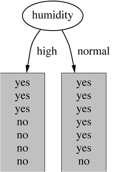
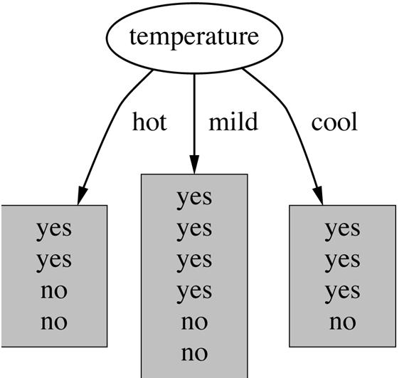
32 Which attribute to select? 32

33 Criterion for attribute selection Which is the best attribute? Want to get the smallest tree Heuristic: choose the attribute that produces the purest nodes Popular impurity criterion: information gain Information gain increases with the average purity of the subsets Strategy: choose attribute that gives greatest information gain 33

34 Computing information Measure information in bits Given a probability distribution, the info required to predict an event is the distribution s entropy Entropy gives the information required in bits (can involve fractions of bits!) Formula for computing the entropy: entropy( p 1, p 2,, p n ) p 1 logp 1 p 2 logp 2 p n logp n 34

Claude Shannon Born: 30 April 1916 Died: 23 February 2001 Father of information theory Claude Shannon, who has died aged 84, perhaps more than anyone laid the groundwork for today s digital

35 Claude Shannon Born: 30 April 1916 Died: 23 February 2001 Father of information theory Claude Shannon, who has died aged 84, perhaps more than anyone laid the groundwork for today s digital revolution. His exposition of information theory, stating that all information could be represented mathematically as a succession of noughts and ones, facilitated the digital manipulation of data without which today s information society would be unthinkable. Shannon s master s thesis, obtained in 1940 at MIT, demonstrated that problem solving could be achieved by manipulating the symbols 0 and 1 in a process that could be carried out automatically with electrical circuitry. That dissertation has been hailed as one of the most significant master s theses of the 20th century. Eight years later, Shannon published another landmark paper, A Mathematical Theory of Communication, generally taken as his most important scientific contribution. Shannon applied the same radical approach to cryptography research, in which he later became a consultant to the US government. Many of Shannon s pioneering insights were developed before they could be applied in practical form. He was truly a remarkable man, yet unknown to most of the world. 35

36 Example: attribute Outlook Outlook = Sunny : info([2,3] ) entropy(2/5,3/5) 2/5log(2/5) 3/ 5log(3/ 5) bits Outlook = Overcast : info([4,0] ) entropy(1,0) 1log(1) 0log(0) 0 bits Outlook = Rainy : info([3,2] ) Note: this is normally undefined. entropy(3/5,2/5) 3/ 5log(3/ 5) 2 / 5log(2 / 5) bits Expected information for attribute: info([3,2],[4,0],[3,2]) (5/14) (4 /14) 0 (5/14) bits 36

37 Computing information gain Information gain: information before splitting information after splitting gain(outlook ) = info([9,5]) info([2,3],[4,0],[3,2]) = = bits Information gain for attributes from weather data: gain(outlook ) = bits gain(temperature ) = bits gain(humidity ) = bits gain(windy ) = bits 37

38 Continuing to split gain(temperature ) = bits gain(humidity ) = bits gain(windy ) = bits 38

39 Final decision tree Note: not all leaves need to be pure; sometimes identical instances have different classes Splitting stops when data can t be split any further 39

40 Wishlist for a purity measure Properties we require from a purity measure: When node is pure, measure should be zero When impurity is maximal (i.e. all classes equally likely), measure should be maximal Measure should obey multistage property (i.e. decisions can be made in several stages): measure([2,3,4]) measure([2,7]) (7/9) measure([3,4]) Entropy is the only function that satisfies all three properties! 40

41 Properties of the entropy The multistage property: q entropy( p,q,r) entropy( p,q r) ( q r) entropy( q r Simplification of computation: info([2,3,4]) Note: instead of maximizing info gain we could just minimize information r, ) q r 2/9log(2/ 9) 3/9log(3/ 9) 4/9log(4/ 9) [ 2log23log3 4log49log9]/9 41

42 Highly-branching attributes Problematic: attributes with a large number of values (extreme case: ID code) Subsets are more likely to be pure if there is a large number of values Information gain is biased towards choosing attributes with a large number of values This may result in overfitting (selection of an attribute that is non-optimal for prediction) Another problem: fragmentation 42

43 Weather data with ID code ID code Outlook Temp. Humidity Windy Play A Sunny Hot High False No B Sunny Hot High True No C Overcast Hot High False Yes D Rainy Mild High False Yes E Rainy Cool Normal False Yes F Rainy Cool Normal True No G Overcast Cool Normal True Yes H Sunny Mild High False No I Sunny Cool Normal False Yes J Rainy Mild Normal False Yes K Sunny Mild Normal True Yes L Overcast Mild High True Yes M Overcast Hot Normal False Yes N Rainy Mild High True No 43

44 Tree stump for ID code attribute Entropy of split: info("id code") info([0,1]) info([0,1]) info([0,1]) 0 bits Information gain is maximal for ID code (namely bits) 44

45 Gain ratio Gain ratio: a modification of the information gain that reduces its bias Gain ratio takes number and size of branches into account when choosing an attribute It corrects the information gain by taking the intrinsic information of a split into account Intrinsic information: entropy of distribution of instances into branches (i.e. how much info do we need to tell which branch an instance belongs to) 45

46 Computing the gain ratio Example: intrinsic information for ID code info([1,1,,1) 14 (1/14 log1/14) bits Value of attribute decreases as intrinsic information gets larger Definition of gain ratio: gain_ratio("attribute") gain("attribute") intrinsic_info("attribute") Example: gain_ratio("id_code") 0.940bits 3.807bits

47 Gain ratios for weather data Outlook Temperature Info: Info: Gain: Gain: Split info: info([5,4,5]) Split info: info([4,6,4]) Gain ratio: 0.247/ Gain ratio: 0.029/ Humidity Windy Info: Info: Gain: Gain: Split info: info([7,7]) Split info: info([8,6]) Gain ratio: 0.152/ Gain ratio: 0.048/

48 More on the gain ratio Outlook still comes out top However: ID code has greater gain ratio Standard fix: ad hoc test to prevent splitting on that type of attribute Problem with gain ratio: it may overcompensate May choose an attribute just because its intrinsic information is very low Standard fix: only consider attributes with greater than average information gain 48

49 Discussion Top-down induction of decision trees: ID3, algorithm developed by Ross Quinlan Gain ratio just one modification of this basic algorithm C4.5: deals with numeric attributes, missing values, noisy data Similar approach: CART There are many other attribute selection criteria! (But little difference in accuracy of result) 49

50 Covering algorithms Convert decision tree into a rule set Straightforward, but rule set overly complex More effective conversions are not trivial Instead, can generate rule set directly for each class in turn find rule set that covers all instances in it (excluding instances not in the class) Called a covering approach: at each stage a rule is identified that covers some of the instances 50

51 Example: generating a rule y b b b b b b b b b x a a a a b b b a a b b y b b b b b b b b b 1 2 a a a a b b b a b a b x y 2 6 b b b b b b b b b 1 2 a a a a b b b a b a b x If true then class = a If x > 1.2 then class = a Possible rule set for class b : If x > 1.2 and y > 2.6 then class = a If x 1.2 then class = b If x > 1.2 and y 2.6 then class = b Could add more rules, get perfect rule set 51

52 Rules vs. trees Corresponding decision tree: (produces exactly the same predictions) But: rule sets can be more perspicuous when decision trees suffer from replicated subtrees Also: in multiclass situations, covering algorithm concentrates on one class at a time whereas decision tree learner takes all classes into account 52

53 Simple covering algorithm Generates a rule by adding tests that maximize rule s accuracy Similar to situation in decision trees: problem of selecting an attribute to split on But: decision tree inducer maximizes overall purity Each new test reduces rule s coverage: space of examples rule so far rule after adding new term 53

54 Selecting a test Goal: maximize accuracy t total number of instances covered by rule p positive examples of the class covered by rule t p number of errors made by rule Select test that maximizes the ratio p/t We are finished when p/t = 1 or the set of instances can t be split any further 54

55 Example: contact lens data Rule we seek: Possible tests: If? then recommendation = hard Age = Young 2/8 Age = Pre-presbyopic 1/8 Age = Presbyopic 1/8 Spectacle prescription = Myope 3/12 Spectacle prescription = Hypermetrope 1/12 Astigmatism = no 0/12 Astigmatism = yes 4/12 Tear production rate = Reduced 0/12 Tear production rate = Normal 4/12 55

56 Modified rule and resulting data Rule with best test added: If astigmatism = yes then recommendation = hard Instances covered by modified rule: Age Spectacle prescription Astigmatism Tear production rate Recommended lenses Young Myope Yes Reduced None Young Myope Yes Normal Hard Young Hypermetrope Yes Reduced None Young Hypermetrope Yes Normal hard Pre-presbyopic Myope Yes Reduced None Pre-presbyopic Myope Yes Normal Hard Pre-presbyopic Hypermetrope Yes Reduced None Pre-presbyopic Hypermetrope Yes Normal None Presbyopic Myope Yes Reduced None Presbyopic Myope Yes Normal Hard Presbyopic Hypermetrope Yes Reduced None Presbyopic Hypermetrope Yes Normal None 56

57 Further refinement Current state: If astigmatism = yes and? then recommendation = hard Possible tests: Age = Young 2/4 Age = Pre-presbyopic 1/4 Age = Presbyopic 1/4 Spectacle prescription = Myope 3/6 Spectacle prescription = Hypermetrope 1/6 Tear production rate = Reduced 0/6 Tear production rate = Normal 4/6 57

58 Modified rule and resulting data Rule with best test added: If astigmatism = yes and tear production rate = normal then recommendation = hard Instances covered by modified rule: Age Spectacle prescription Astigmatism Tear production rate Recommended lenses Young Myope Yes Normal Hard Young Hypermetrope Yes Normal hard Pre-presbyopic Myope Yes Normal Hard Pre-presbyopic Hypermetrope Yes Normal None Presbyopic Myope Yes Normal Hard Presbyopic Hypermetrope Yes Normal None 58

59 Further refinement Current state: Possible tests: If astigmatism = yes and tear production rate = normal and? then recommendation = hard Age = Young 2/2 Age = Pre-presbyopic 1/2 Age = Presbyopic 1/2 Spectacle prescription = Myope 3/3 Spectacle prescription = Hypermetrope 1/3 Tie between the first and the fourth test We choose the one with greater coverage 59

60 The result Final rule: If astigmatism = yes and tear production rate = normal and spectacle prescription = myope then recommendation = hard Second rule for recommending hard lenses : (built from instances not covered by first rule) If age = young and astigmatism = yes and tear production rate = normal then recommendation = hard These two rules cover all hard lenses : Process is repeated with other two classes 60

Pseudo-code for PRISM For each class C Initialize E to the instance set While E contains instances in class C Create a rule R with an empty left-hand side that predicts class C Until R is perfect (or

61 Pseudo-code for PRISM For each class C Initialize E to the instance set While E contains instances in class C Create a rule R with an empty left-hand side that predicts class C Until R is perfect (or there are no more attributes to use) do For each attribute A not mentioned in R, and each value v, Consider adding the condition A = v to the left-hand side of R Select A and v to maximize the accuracy p/t (break ties by choosing the condition with the largest p) Add A = v to R Remove the instances covered by R from E 61

62 Rules vs. decision lists PRISM with outer loop removed generates a decision list for one class Subsequent rules are designed for rules that are not covered by previous rules But: order doesn t matter because all rules predict the same class Outer loop considers all classes separately No order dependence implied Problems: overlapping rules, default rule required 62

63 Separate and conquer Methods like PRISM (for dealing with one class) are separate-and-conquer algorithms: First, identify a useful rule Then, separate out all the instances it covers Finally, conquer the remaining instances Difference to divide-and-conquer methods: Subset covered by rule doesn t need to be explored any further 63

64 Association rules Association rules can predict any attribute and combinations of attributes are not intended to be used together as a set Problem: immense number of possible associations Output needs to be restricted to show only the most predictive associations only those with high support and high confidence 64

65 Support and confidence of a rule Support: number of instances predicted correctly Confidence: number of correct predictions, as proportion of all instances the rule applies to Example: 4 cool days with normal humidity If temperature = cool then humidity = normal Support = 4, confidence = 100% Normally: minimum support and confidence pre-specified (e.g. 58 rules with support 2 and confidence 95% for weather data) 65

66 Support and confidence of a rule Support: number of instances predicted correctly Confidence: number of correct predictions, as proportion of all instances the rule applies to Example: 4 cool days with normal humidity Sunny Mild Normal True Yes If temperature = cool then humidity = normal Overcast Mild High True Yes Support = 4, confidence = 100% Outlook Temp Humidity Windy Play Sunny Hot High False No Sunny Hot High True No Overcast Hot High False Yes Rainy Mild High False Yes Rainy Cool Normal False Yes Rainy Cool Normal True No Overcast Cool Normal True Yes Sunny Mild High False No Sunny Cool Normal False Yes Rainy Mild Normal False Yes Overcast Hot Normal False Yes Normally: minimum support and confidence pre-specified (e.g. 58 rules with support 2 and confidence 95% for weather data) Rainy Mild High True No 66

67 Interpreting association rules Interpretation is not obvious: If windy = false and play = no then outlook = sunny and humidity = high is no the same as If windy = false and play = no then outlook = sunny If windy = false and play = no then humidity = high However, it means that the following also holds: If humidity = high and windy = false and play = no then outlook = sunny 67

68 Mining association rules Naïve method for finding association rules: Use separate-and-conquer method Treat every possible combination of attribute values as a separate class Two problems: Computational complexity Resulting number of rules (which would have to be pruned on the basis of support and confidence) But: we can look for high support rules directly! 68

69 Item sets Support: number of instances correctly covered by association rule The same as the number of instances covered by all tests in the rule (LHS and RHS!) Item: one test/attribute-value pair Item set : all items occurring in a rule Goal: only rules that exceed pre-defined support Do it by finding all item sets with the given minimum support and generating rules from them! 69

70 Item sets for weather data One-item sets Two-item sets Three-item sets Four-item sets Outlook = Sunny (5) Outlook = Sunny Outlook = Sunny Outlook = Sunny Temperature = Hot (2) Temperature = Hot Temperature = Hot Humidity = High (2) Humidity = High Play = No (2) Temperature = Cool (4) Outlook = Sunny Outlook = Sunny Outlook = Rainy Humidity = High (3) Humidity = High Temperature = Mild Windy = False (2) Windy = False Play = Yes (2) In total: 12 one-item sets, 47 two-item sets, 39 three-item sets, 6 four-item sets and 0 five-item sets (with minimum support of two) 70

71 Item sets for weather data One-item sets Two-item sets Three-item sets Four-item sets Outlook = Sunny (5) Temperature = Cool (4) Outlook = Sunny Temperature = Hot (2) Outlook = Sunny Humidity = High (3) Outlook Temp Humidity Windy Play Sunny Hot High False No Sunny Hot High True No Overcast Hot High False Yes Rainy Mild High False Yes Rainy Cool Normal False Yes Outlook = Sunny Temperature = Hot Humidity = High (2) Outlook = Sunny Humidity = High Windy = False (2) Outlook = Sunny Temperature = Hot Humidity = High Play = No (2) Rainy Cool Normal True No Overcast Cool Normal True Yes Sunny Mild High False No Sunny Cool Normal False Yes Outlook = Rainy Temperature = Mild Windy = False Play = Yes (2) Rainy Mild Normal False Yes Sunny Mild Normal True Yes Overcast Mild High True Yes Overcast Hot Normal False Yes Rainy Mild High True No In total: 12 one-item sets, 47 two-item sets, 39 three-item sets, 6 four-item sets and 0 five-item sets (with minimum support of two) 71

72 Generating rules from an item set Once all item sets with minimum support have been generated, we can turn them into rules Example: Humidity = Normal, Windy = False, Play = Yes (4) Seven (2 N -1) potential rules: If Humidity = Normal and Windy = False then Play = Yes If Humidity = Normal and Play = Yes then Windy = False If Windy = False and Play = Yes then Humidity = Normal If Humidity = Normal then Windy = False and Play = Yes If Windy = False then Humidity = Normal and Play = Yes If Play = Yes then Humidity = Normal and Windy = False If True then Humidity = Normal and Windy = False and Play = Yes 4/4 4/6 4/6 4/7 4/8 4/9 4/12 72

73 Rules for weather data Rules with support > 1 and confidence = 100%: Association rule Sup. Conf. 1 Humidity=Normal Windy=False Play=Yes 4 100% 2 Temperature=Cool Humidity=Normal 4 100% 3 Outlook=Overcast Play=Yes 4 100% 4 Temperature=Cold Play=Yes Humidity=Normal 3 100% Outlook=Sunny Temperature=Hot Humidity=High 2 100% In total: 3 rules with support four 5 with support three 50 with support two 73

74 Example rules from the Item set: same set Temperature = Cool, Humidity = Normal, Windy = False, Play = Yes (2) Resulting rules (all with 100% confidence): Temperature = Cool, Windy = False Humidity = Normal, Play = Yes Temperature = Cool, Windy = False, Humidity = Normal Play = Yes Temperature = Cool, Windy = False, Play = Yes Humidity = Normal due to the following frequent item sets: Temperature = Cool, Windy = False (2) Temperature = Cool, Humidity = Normal, Windy = False (2) Temperature = Cool, Windy = False, Play = Yes (2) 74

75 Generating item sets efficiently How can we efficiently find all frequent item sets? Finding one-item sets easy Idea: use one-item sets to generate twoitem sets, two-item sets to generate threeitem sets, If (A B) is frequent item set, then (A) and (B) have to be frequent item sets as well! In general: if X is frequent k-item set, then all (k-1)-item subsets of X are also frequent Compute k-item set by merging (k-1)-item sets 75

76 Example Given: five three-item sets (A B C), (A B D), (A C D), (A C E), (B C D) Lexicographically ordered! Candidate four-item sets: (A B C D) OK because of (B C D) (A C D E) Not OK because of (C D E) Final check by counting instances in dataset! (k 1)-item sets are stored in hash table 76

77 Generating rules efficiently We are looking for all high-confidence rules Support of antecedent obtained from hash table But: brute-force method is (2 N -1) Better way: building (c + 1)-consequent rules from c-consequent ones Observation: (c + 1)-consequent rule can only hold if all corresponding c-consequent rules also hold Resulting algorithm similar to procedure for large item sets 77

78 Example 1-consequent rules: If Outlook = Sunny and Windy = False and Play = No then Humidity = High (2/2) If Humidity = High and Windy = False and Play = No then Outlook = Sunny (2/2) Corresponding 2-consequent rule: If Windy = False and Play = No then Outlook = Sunny and Humidity = High (2/2) Final check of antecedent against hash table! 78

79 Association rules: discussion Above method makes one pass through the data for each different size item set Other possibility: generate (k+2)-item sets just after (k+1)-item sets have been generated Result: more (k+2)-item sets than necessary will be considered but less passes through the data Makes sense if data too large for main memory Practical issue: generating a certain number of rules (e.g. by incrementally reducing min. support) 79

80 Other issues Standard ARFF format very inefficient for typical market basket data Attributes represent items in a basket and most items are usually missing Need way of representing sparse data Instances are also called transactions Confidence is not necessarily the best measure Example: milk occurs in almost every supermarket transaction Other measures have been devised (e.g. lift) 80

81 Linear models Work most naturally with numeric attributes Standard technique for numeric prediction: linear regression Outcome is linear combination of attributes x w0 w1a 1 w2a2... w k a k Weights are calculated from the training data Predicted value for first training instance a (1) (1) (1) (1) w0 a0 w1a 1 w2a2... w a k (1) k k j0 w j a (1) j 81

82 Minimizing the squared error Choose k +1 coefficients to minimize the squared error on the training data 2 n Squared error: k x i1 j0 Derive coefficients using standard matrix operations Can be done if there are more instances than attributes (roughly speaking) Minimizing the absolute error is more difficult ( i) w a j ( i) j 82

83 Classification Any regression technique can be used for classification Training: perform a regression for each class, setting the output to 1 for training instances that belong to class, and 0 for those that don t Prediction: predict class corresponding to model with largest output value (membership value) For linear regression this is known as multiresponse linear regression 83

84 84 Theoretical justification } ) ) ( {( 2 x X Y X f E y } ) ) 1 ( ) 1 ( ) ( {( 2 x X Y x X Y P x X Y P X f E y } ) ) 1 ( {( }) { ) 1 ( ( )) 1 ( ) ( ( 2 )) 1 ( ) ( ( 2 2 x X Y x X Y P E x X Y E x X Y P x X Y P x f x X Y P x f y y } ) ) 1 ( {( } ) 1 ( { )) 1 ( ) ( ( 2 )) 1 ( ) ( ( 2 2 x X Y x X Y P E x X Y x X Y P E x X Y P x f x X Y P x f y y } ) ) 1 ( {( )) 1 ( ) ( ( 2 2 x X Y x X Y P E x X Y P x f y Model Instance Observed target value (either 0 or 1) True class probability Constant We want to minimize this The scheme minimizes this

85 Pairwise regression Another way of using regression for classification: A regression function for every pair of classes, using only instances from these two classes Assign output of +1 to one member of the pair, 1 to the other Prediction is done by voting Class that receives most votes is predicted Alternative: don t know if there is no agreement More likely to be accurate but more expensive 85

86 Logistic regression Problem: some assumptions violated when linear regression is applied to classification problems Logistic regression: alternative to linear regression Designed for classification problems Tries to estimate class probabilities directly Does this using the maximum likelihood method Uses this linear model: P log w 1 P 0 a 0 w 1 a 1 w 2 a 2 w k a k Class probability 86

87 Discussion of linear models Not appropriate if data exhibits non-linear dependencies But: can serve as building blocks for more complex schemes (i.e. model trees) Example: multi-response linear regression defines a hyperplane for any two given classes: (w (1) 0 w (2) 0 )a 0 (w (1) 1 w (2) 1 )a 1 (w (1) 2 w (2) 2 )a 2 (w (1) k w (2) k )a k 0 87

Instance-based representation Simplest form of learning: rote learning Training instances are searched for instance that most closely resembles new instance The instances themselves

88 Instance-based representation Simplest form of learning: rote learning Training instances are searched for instance that most closely resembles new instance The instances themselves represent the knowledge Also called instance-based learning Similarity function defines what s learned Instance-based learning is lazy learning Methods: nearest-neighbor k-nearest-neighbor 88

89 The distance function Simplest case: one numeric attribute Distance is the difference between the two attribute values involved (or a function thereof) Several numeric attributes: normally, Euclidean distance is used and attributes are normalized Nominal attributes: distance is set to 1 if values are different, 0 if they are equal Are all attributes equally important? Weighting the attributes might be necessary 89

90 Instance-based learning Distance function defines what s learned Most instance-based schemes use Euclidean distance: (1) (2) 2 (1) (2) 2 (1) (2) 2 ( a1 a1 ) ( a2 a2 )... ( a k ak ) a (1) and a (2) : two instances with k attributes Taking the square root is not required when comparing distances Other popular metric: city-block metric Adds differences without squaring them 90

91 Normalization and other issues Different attributes are measured on different scales need to be normalized: a i vi min vi maxv min v v i : the actual value of attribute i Nominal attributes: distance either 0 or 1 Common policy for missing values: assumed to be maximally distant (given normalized attributes) i i 91

92 Discussion of 1-NN Often very accurate but slow: simple version scans entire training data to derive a prediction Assumes all attributes are equally important Remedy: attribute selection or weights Possible remedies against noisy instances: Take a majority vote over the k nearest neighbors Removing noisy instances from dataset (difficult!) Statisticians have used k-nn since early 1950s If n and k/n 0, error approaches minimum 92

93 Clustering Clustering techniques apply when there is no class to be predicted Aim: divide instances into natural groups As we have seen clusters can be: disjoint vs. overlapping deterministic vs. probabilistic flat vs. hierarchical We will look at a classic algorithm called k-means k-means clusters are disjoint, deterministic, and flat 93

94 The k-means algorithm To cluster data into k groups: (k is predefined) 1. Choose k cluster centers e.g. at random 2. Assign instances to clusters based on distance to cluster centers 3. Compute centroids of clusters 4. Go to step 1 until convergence 94

95 Discussion Algorithm minimizes squared distance to cluster centers Result can vary significantly based on initial choice of seeds Can get trapped in local minimum Example: instances initial cluster centers To increase chance of finding global optimum: restart with different random seeds Can we applied recursively with k=2 95

96 Comments on basic methods Bayes rule stems from his Essay towards solving a problem in the doctrine of chances (1763) Difficult bit: estimating prior probabilities Extension of Naïve Bayes: Bayesian Networks Algorithm for association rules is called APRIORI Minsky and Papert (1969) showed that linear classifiers have limitations, e.g. can t learn XOR But: combinations of them can ( Neural Nets) 96

Slides for Data Mining by I. H. Witten and E. Frank

Slides for Data Mining by I. H. Witten and E. Frank 4 Algorithms: The basic methods Simplicity first: 1R Use all attributes: Naïve Bayes Decision trees: ID3 Covering algorithms: decision rules: PRISM Association