Chapter 5: Forecasting

Transcription

1 1 Textbook: pp Chapter 5: Forecasting Every day, managers make decisions without knowing what will happen in the future

2 2 Learning Objectives After completing this chapter, students will be able to: Understand and know when to use various families of forecasting models Compare moving averages, exponential smoothing, and other time-series models Calculate measures of forecast accuracy Apply forecast models for random variations Apply forecast models for trends and random variations Manipulate data to account for seasonal variations Apply forecast models for trends, seasonal variations, and random variations Explain how to monitor and control forecasts

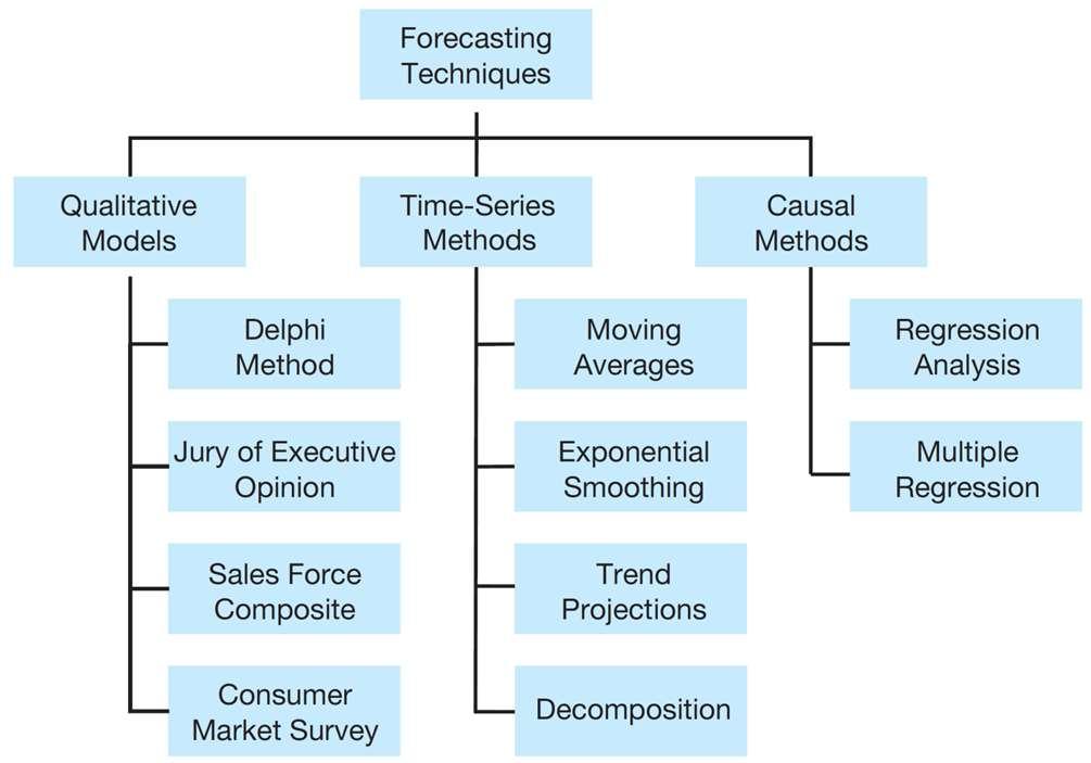
3 3 Introduction Main purpose of forecasting: Managers are trying to reduce uncertainty and make better estimates of what will happen in the future! Subjective methods Seat-of-the pants methods - intuition, experience More formal quantitative (e.g. least squares regression analysis, trend projections ) and qualitative techniques

4 Forecasting Models 4

5 5 Qualitative Models (1 of 3) Incorporate judgmental or subjective factors o Useful when subjective factors are important or accurate quantitative data is difficult to obtain Common qualitative techniques 1. Delphi method 2. Jury of executive opinion 3. Sales force composite 4. Consumer market surveys

6 6 Qualitative Models (2 of 3) Delphi Method o Iterative group process o Respondents provide input to decision makers o Repeated until consensus is reached Jury of Executive Opinion o Collects opinions of a small group of high-level managers o May use statistical models for analysis

7 7 Qualitative Models (3 of 3) Sales Force Composite o Allows individual salespersons estimates o Reviewed for reasonableness o Data is compiled at a district or national level Consumer Market Survey o Information on purchasing plans solicited from customers or potential customers o Used in forecasting, product design, new product planning

8 8 Time-Series Models Predict the future based on the past Uses only historical data on one variable Extrapolations of past values of a series If we are forecasting weekly sales for fidget spinners, we use the past weekly sales for fidget spinners in making the forecast for future sales ignoring other factors such as the economy, competition, and even the selling price of the fidget spinners.

9 9 Components of a Time Series (1 of 4) Sequence of values recorded at successive intervals of time (e.g. weekly sales of Lenovo tablet computers; quarterly earnings reports of Air China ) Four possible components o Trend (T) o Seasonal (S) o Cyclical (C) o Random (R)

10 10 Components of a Time Series (2 of 4) 1. Trend (T) is the gradual upward or downward movement of the data over time. 2. Seasonality (S) is a pattern of the demand fluctuation above or below the trend line that repeats at regular intervals. 3. Cycles (C) are patterns in annual data that occur every several years. They are usually tied into the business cycle (used only in very long forecasts!) 4. Random variations (R) are blips in the data caused by chance and unusual situations; they follow no discernible pattern.

11 11 Components of a Time Series (3 of 4) Scatter Diagram for Four Time Series of Quarterly Data:

12 12 Components of a Time Series (4 of 4) Scatter Diagram of a Time Series with Cyclical and Random Components:

13 13 Trend (T); Seasonal (S); Cyclical (C); Random (R) Time-Series Models Two basic forms: Multiplicative (multiplies the components to provide an estimate) Demand = T S C R Additive (adds the components together to provide an estimate) Demand = T + S + C + R Combinations are possible

14 Naïve model does not attempt to address any of the components of a time series. A naïve forecast for the next time period is the actual value that was observed in the current time period. 14 Measures of Forecast Accuracy (1 of 4) Compare forecasted values with actual values o See how well one model works o To compare models deviation Forecast error = Actual value Forecast value One measure of accuracy is the o Mean absolute deviation (MAD): forecast error MAD n sum of the absolute values of the individual forecast errors number of errors (n)

15 Absolute value X of a real number X is the non-negative value of X without regard to its sign. 15 Measures of Forecast Accuracy (2 of 4) MAD Computing the Mean Absolute Deviation (MAD): forecast error n This means that on average each forecast missed the actual value by 17.8 units!

16 16 Measures of Forecast Accuracy (3 of 4) Computing the Mean Absolute Deviation (MAD): Forecast based on naïve model No attempt to adjust for time series components

17 * Bias may be negative or positive Not a good measure of the actual size of the errors because the negative errors can cancel out the positive errors! 17 Measures of Forecast Accuracy (4 of 4) Other common measures: o Mean squared error (MSE) 2 (error) MSE n o Mean absolute percent error (MAPE) error actual MAPE 100% n o Bias is the average error and tells whether the forecast tends to be too high or too low and by how much*!

18 18 Forecasting Random Variations If all variations in a time series are due to random variations [no trend / seasonal / cyclical component is present] some type of averaging or smoothing model would be appropriate! Averaging techniques smooth out forecasts and will not be too heavily influenced by random variations: o Moving averages o Weighted moving averages o Exponential smoothing

19 19 n = number of periods to average Moving Averages (1 of 3) Used when demand is relatively steady over time o The next forecast is the average of the most recent n data values from the time series o Smooths out short-term irregularities in the data series Moving average forecast = Sum of demands in previous n n periods Example Four-month moving average : Found by summing the demand during the past four months and dividing by 4. With each passing month, the most recent month s data are added to the sum of the previous three months data, and the earliest month is dropped smoothes out irregularities!

20 20 Moving Averages (2 of 3) Mathematically: F t 1 Y Y... Y t t 1 t n 1 n where F t+1 = forecast for time period t + 1 Y t n = actual value in time period t = number of periods to average

21 21 n = number of periods to average Wallace Garden Supply (1 of 4) Wallace Garden Supply wants to forecast demand for its Storage Shed o Collected data for the past year o Use a three-month moving average (n = 3) and forecast sales for the next January! F t 1 Y Y... Y t t 1 t n 1 n

22 22 n = number of periods to average Wallace Garden Supply --- Shed Sales (2 of 4) F t 1 Y Y... Y n t t 1 t n 1

23 23 n = number of periods to average Wallace Garden Supply --- Shed Sales (2 of 4) F t 1 Y Y... Y n t t 1 t n 1

24 24 Moving Averages (3 of 3) A simple moving average gives the same weight to each of the past observations being used to develop the forecast. F t 1 Y Y... Y n t t 1 t n 1

25 25 Weighted Moving Averages Weighted moving averages use weights to put more emphasis on previous periods Often used when a trend or other pattern is emerging Ft 1 Mathematically (Weight in period i)(actual value in period i) (Weights) F t 1 w Y w Y... w Y 1 t 2 t 1 n t n 1 w w... w 1 2 n where w i = weight for the i th observation

26 26 Wallace Garden Supply (3 of 4) Use a 3-month weighted moving average model to forecast demand Weighting scheme:

27 Weights of 3 for the most recent observation, 2 for the next observation, and 1 for the most distant observation. The sum of weights is 6! 27 Wallace Garden Supply (4 of 4) 1 t 2 t 1 n t n 1 Weighted Moving Average Forecast for Wallace Garden Supply: F t 1 w Y w Y... w Y w w... w 1 2 n

28 28 Wallace Garden Supply (4 of 4) 1 t 2 t 1 n t n 1 Weighted Moving Average Forecast for Wallace Garden Supply: F t 1 w Y w Y... w Y w w... w 1 2 n

29 29 Exponential Smoothing (1 of 2) Exponential smoothing: o A type of moving average o Easy to use o Requires little record keeping of data New forecast = Last period s forecast + α(last period s actual demand Last period s forecast) α is a weight (or smoothing constant) with a value 0 α 1

30 30 Smoothing constant (α), can be changed to give more weight to recent data when the value is high or more weight to past data when it is low! Exponential Smoothing (2 of 2) Mathematically F 1 F ( Y F ) t t t t where F t+1 = new forecast (for time period t + 1) F t = pervious forecast (for time period t) α = smoothing constant (0 α 1) Y t = pervious period s actual demand The idea is simple the new estimate is the old estimate plus some fraction of the error in the last period!

31 31 Smoothing constant (α) is low --- more weight to past data is given. Exponential Smoothing Example (1 of 2) In January, February s demand for a certain car model was predicted to be 142 Actual February demand was 153 autos Using a smoothing constant of α = 0.20, what is the forecast for March? New forecast (for March demand) = F t 1 F t ( Y t Ft )

32 32 Exponential Smoothing Example (1 of 2) In January, February s demand for a certain car model was predicted to be 142 Actual February demand was 153 autos Using a smoothing constant of α = 0.20, what is the forecast for March? New forecast (for March demand) = ( ) = or 144 autos If actual March demand = 136 New forecast (for April demand) = F t 1 F t ( Y t Ft )

33 33 Exponential Smoothing Example (1 of 2) In January, February s demand for a certain car model was predicted to be 142 Actual February demand was 153 autos Using a smoothing constant of α = 0.20, what is the forecast for March? New forecast (for March demand) = ( ) = or 144 autos If actual March demand = 136 New forecast (for April demand) = ( ) = or 143 autos

34 34 Exponential Smoothing Example (2 of 2) Selecting the appropriate value for our smoothing constant α is key to obtaining a good forecast The objective is always to generate an accurate forecast (only the correct α delivers this result!) The general approach is to develop trial forecasts with different values of α and select the α that results in the lowest Mean Absolute Deviation (MAD). MAD forecast error n

35 F 1 F ( Y F ) t t t t 35 Port of Baltimore Example (1 of 3) Let us apply this concept with a trial-and-error testing of two values of α = 0.1 and = 0.5 in an example. The port of Baltimore has unloaded large quantities of grain from ships during the past eight quarters. The port s operations manager wants to test the use of exponential smoothing to see how well the technique works in predicting tonnage unloaded. He assumes that the forecast of grain unloaded in the first quarter was 175 tons. exponential smoothing model is used for the first time --- a previous value for a forecast must be assumed!

36 F 1 F ( Y forecast error F ) MAD t t t t n 36 Port of Baltimore Example (2 of 3) Port of Baltimore Exponential Smoothing: Forecasts for α = 0.10 and α = 0.50

37 37 n = number of errors (n) Port of Baltimore Example (3 of 3) Absolute Deviations and MADs for the Port of Baltimore Example:

38 38 PROGRAMME 5.1A Using Software (1 of 7) F t 1 w Y w Y... w Y 1 t 2 t 1 n t n 1 w w... w 1 2 n Selecting the Forecasting Model in Wallace Garden Supply Problem: Weighted moving average

39 Weights of 3 for the most recent observation, 2 for the next observation, and 1 for the most distant observation. The sum of weights is 6! 39 Wallace Garden Supply (4 of 4) 1 t 2 t 1 n t n 1 Weighted Moving Average Forecast for Wallace Garden Supply: F t 1 w Y w Y... w Y w w... w 1 2 n

40 40 PROGRAMME 5.1B Using Software (2 of 7) Initialising Excel QM Spreadsheet for Wallace Garden Supply Problem:

41 41 PROGRAMME 5.1C Using Software (3 of 7) Excel QM Output for Wallace Garden Supply Problem:

42 42 PROGRAMME 5.2A Using Software (4 of 7) Selecting Time-Series Analysis in QM for Windows in the Forecasting Module:

43 43 PROGRAMME 5.2B Using Software (5 of 7) Entering Data for Port of Baltimore Example in QM for Windows:

44 44 PROGRAMME 5.2C Using Software (6 of 7) Selecting the Model and Entering Data for Port of Baltimore Example in QM for Windows:

45 45 PROGRAMME 5.2D Using Software (7 of 7) Output for Port of Baltimore Example in QM for Windows:

46 Trend (T) is the gradual upward or downward movement of the data over time. 46 Forecasting Models Trend and Random Variations Exponential smoothing does not respond to trends If there is a trend present in a time series, the forecasting model must account for this and cannot simply average past values! A more complex model can be used The basic idea is o Develop an exponential smoothing forecast, and o Adjust it for the trend!

47 Smoothing constant for forecast: alpha (α) Smoothing constant for trend: beta (β) 47 Exponential Smoothing with Trend (1 of 2) The equation for the trend correction uses a new smoothing constant β F t and T t must be given or estimated Three steps in developing FIT t forecast including trend Step 1: Compute smoothed forecast F t+1 Smoothed forecast = Previous forecast including trend + α(last error) F t 1 FIT t ( Y t FITt )

48 Smoothing constant for forecast: alpha (α) Smoothing constant for trend: beta (β) 48 Exponential Smoothing with Trend (2 of 2) Step 2: Update the trend (T t +1 ) using Smoothed forecast = Previous forecast including trend + β(error or excess in trend) T T ( F FIT ) t 1 t t 1 t Step 3: Calculate the trend-adjusted exponential smoothing forecast (FIT t +1 ) using Forecast including trend (FIT t+1 ) = Smoothed forecast (F t+1 ) + Smoothed trend (T t+1 ) FIT F T t 1 t 1 t 1

49 Smoothing constant for forecast: alpha (α) Smoothing constant for trend: beta (β) 49 Selecting a Smoothing Constant A high value of β makes the forecast more responsive to changes in trend T T ( F FIT ) t 1 t t 1 t A low value of β gives less weight to the recent trend and tends to smooth out the trend Values are often selected using a trial-and-error approach based on the value of the Mean Absolute Deviation (MAD) for different values of β

50 Smoothing constant for forecast: alpha (α) Smoothing constant for trend: beta (β) 50 Midwestern Manufacturing (1 of 6) Demand for electrical generators from o Midwest assumes F 1 is perfect, T 1 = 0, α = 0.3, β = 0.4 FIT 1 = F 1 +T 1 = 74+0 = 74 Midwestern Manufacturing s Demand:

51 51 F 1 is perfect, T 1 = 0, α = 0.3, β = 0.4 Midwestern Manufacturing (2 of 6) F t 1 FIT t ( Y t FITt ) For 2008 (time period 2) Step 1: Compute F t+1 F 2 = FIT 1 + α(y 1 FIT 1 ) = Step 2: Update the trend T T ( F FIT ) t 1 t t 1 t T 2 = T 1 + β(f 2 FIT 1 ) =

52 52 F 1 is perfect, T 1 = 0, α = 0.3, β = 0.4 Midwestern Manufacturing (2 of 6) F t 1 FIT t ( Y t FITt ) For 2008 (time period 2) Step 1: Compute F t+1 F 2 = FIT 1 + α(y 1 FIT 1 ) = (74 74) = 74 Step 2: Update the trend T T ( F FIT ) t 1 t t 1 t T 2 = T 1 + β(f 2 FIT 1 ) =

53 53 F 1 is perfect, T 1 = 0, α = 0.3, β = 0.4 Midwestern Manufacturing (2 of 6) For 2008 (time period 2) Step 1: Compute F t+1 F 2 = FIT 1 + α(y 1 FIT 1 ) = (74 74) = 74 Step 2: Update the trend T 2 = T 1 + β(f 2 FIT 1 ) = 0 +.4(74 74) = 0

54 54 Midwestern Manufacturing (3 of 6) Step 3: Calculate the trend-adjusted exponential smoothing forecast (F t+1 ) using FIT F T t 1 t 1 t 1 FIT 2 = F 2 + T 2 =

55 55 Midwestern Manufacturing (3 of 6) Step 3: Calculate the trend-adjusted exponential smoothing forecast (F t+1 ) using FIT 2 = F 2 + T 2 = = 74 FIT 2 = 74, T 2 = 0

56 F 1 is perfect, T 1 = 0, α = 0.3, β = 0.4 FIT 2 = 74, T 2 = 0 56 Midwestern Manufacturing (4 of 6) For 2009 (time period 3) Step 1: F 3 = FIT 2 + α(y 2 FIT 2 ) = Step 2: T 3 = T 2 + β(f 3 FIT 2 ) F 1 FIT ( Y FIT ) t t t t T T ( F FIT ) t 1 t t 1 t = Step 3: FIT 3 = F 3 + T 3 FIT F T t 1 t 1 t 1 =

57 F 1 is perfect, T 1 = 0, α = 0.3, β = 0.4 FIT 2 = 74, T 2 = 0 57 Midwestern Manufacturing (4 of 6) For 2009 (time period 3) Step 1: F 3 = FIT 2 + α(y 2 FIT 2 ) = (79 74) = 75.5 Step 2: T 3 = T 2 + β(f 3 FIT 2 ) F 1 FIT ( Y FIT ) t t t t T T ( F FIT ) t 1 t t 1 t = 0 +.4( ) = 0.6 Step 3: FIT 3 = F 3 + T 3 FIT F T t 1 t 1 t 1 = = 76.1

58 58 Midwestern Manufacturing (5 of 6) Midwestern Manufacturing Exponential Smoothing with Trend Forecasts:

59 59 PROGRAMME 5.3 Midwestern Manufacturing (6 of 6) Output from Excel QM in Excel 2016 for Trend-Adjusted Exponential Smoothing Example:

60 60 Trend Projections (1 of 2) Fits a trend line to a series of historical data points and then projects the line into the future for medium- to longrange forecasts Trend equations can be developed based on exponential or quadratic models Linear model developed using regression analysis is simplest A trend line is simply a linear regression equation in which the independent variable (X) is the time period. Yˆ b b X 0 1

61 61 Trend Projections (2 of 2) Mathematical formula: Yˆ b b X 0 1 where Ŷ = predicted value b 0 b 1 = intercept = slope of the line X = time period (i.e., X = 1, 2, 3,, n)

62 62 Midwestern Manufacturing (1 of 4) Based on least squares regression, the forecast equation is Year 2014 is coded as X = 8 For X = 9 Yˆ X (sales in 2014)= (8) = , or 141 generators (sales in 2015)= (9) = , or 152 generators

63 63 PROGRAMME 5.4 Midwestern Manufacturing (2 of 4) Output from Excel QM in Excel 2016 for Trend Line Example:

64 64 PROGRAMME 5.5 Midwestern Manufacturing (3 of 4) Output from QM for Windows for Trend Line Example:

65 65 Midwestern Manufacturing (4 of 4) Generator Demand and Projections for Next Three Years Based on Trend Line:

66 Analysing data in monthly or quarterly terms makes it easy to spot seasonal patterns! 66 Seasonal Variations Example: Demand for coal and fuel oil usually peaks during the cold winter months. Recurring variations over time may indicate the need for seasonal adjustments in the trend line A seasonal index indicates how a particular season compares with an average season o An index of 1 indicates an average season When no trend is present, the index can be found by dividing the average value for a particular season by the average of all the data o An index > 1 indicates the season is higher than average o An index < 1 indicates a season lower than average

67 67 Seasonal Indices Each observation in the time series is divided by the appropriate seasonal index to remove the impact of the seasonality Deseasonalised data is created! Once deseasonalised forecasts have been developed, values are multiplied by the seasonal indices Seasonal indices are computed in two ways: o Overall average (when no trend is present) o Centered-moving-average approach (when trend is present)

68 68 An index of 1 means the season is average! Seasonal Indices with No Trend (1 of 3) Divide average value for each season by the average of all data o Telephone answering machines at Eichler Supplies o Sales data for the past two years for one model o Create a forecast that includes seasonality

69 69 Seasonal Indices with No Trend (2 of 3) First: The average demand in each month is computed. Answering Machine Sales and Seasonal Indices: ( ) /2 = = 90 / 94

70 70 An index of 1 means the season is average! Seasonal Indices with No Trend (3 of 3) Calculations for the seasonal indices: Let s now suppose we expected the third year s annual demand to be 1,200 units!

71 71 Seasonal Indices with Trend (1 of 2) When both trend and seasonal components are present in a time series, a change from one month to the next could be due to a trend, to a seasonal variation, or simply to random fluctuations. Centered moving average (CMA) approach prevents trend being interpreted as seasonal New example: Turner Industries sales contain both trend and seasonal components

72 72 Turner Industries (1 of 7) Quarterly Sales ($1,000,000s) for Turner Industries: Can you identify any trend or seasonal components?

73 73 Seasonal Indices with Trend (2 of 2) Steps in Centered moving average (CMA): 1. Compute the CMA for each observation (where possible) e.g. quarter 3 of year 1 2. Compute the seasonal ratio = Observation CMA for that observation 3. Average seasonal ratios to get seasonal indices 4. If seasonal indices do not add to the number of seasons, multiply each index by (Number of seasons) (Sum of indices)

74 74 Contains trend and seasonal components! Turner Industries (2 of 7) Quarterly Sales ($1,000,000s) for Turner Industries:

75 75 Turner Industries (3 of 7) To calculate the CMA for quarter 3 of year 1, compare the actual sales (150) with an average quarter centred on that time period Centre is Q3 We have a total of 4 quarters (1 year data) but we need an equal number of quarters before and after the quarter 3 so the trend is averaged out! Use 1.5 quarters before quarter 3 and 1.5 quarters after quarter 3 o Take quarters 2, 3, and 4 and one half of quarters 1, year 1 and quarter 1, year 2 CMA(q3, y1) = 0.5(108) (116) 4 = 132.0

76 76 Turner Industries (4 of 7) Compare the actual sales in quarter 3 to the centered moving average (CMA) to find the seasonal ratio: Seasonal ratio = Sales in quarter 3 CMA = =1.136 CMA (q3, y1) = 132

77 77 Turner Industries (5 of 7) What does this ratio say? Interpretation? Centered Moving Averages and Seasonal Ratios for Turner Industries:

78 78 Turner Industries (5 of 7) Sales in Q3 of Year 1 are about 13.6% higher than an average quarter! Centered Moving Averages and Seasonal Ratios for Turner Industries: We now have two seasonal indices for Q3 (year 1 and year 2)

79 If the sum were not 4, an adjustment would be made. We would multiply each index by 4 and divide this by the sum of the indices. 79 Turner Industries (6 of 7) The two seasonal ratios for each quarter are averaged to get the seasonal index: Index for quarter 1 = I 1 = ( ) 2 = 0.85 Index for quarter 2 = I 2 = ( ) 2 = 0.96 Index for quarter 3 = I 3 = ( ) 2 = 1.13 Index for quarter 4 = I 4 = ( ) 2 = 1.06 The sum of these indices should be the number of seasons (4) since an average season should have an index of 1.

80 80 Turner Industries (7 of 7) Contrast CMA plot and original data? Do you see a definite trend? Scatterplot of Turner Industries Sales Data and Centered Moving Average:

81 81 Trend, Seasonal, and Random Variations The Decomposition method isolates the linear trend and seasonal factors to develop more accurate forecasts Five steps to decomposition: 1. Compute seasonal indices using CMAs 2. Deseasonalise the data by dividing each number by its seasonal index 3. Find the equation of a trend line using the deseasonalised data 4. Forecast for future periods using the trend line 5. Multiply the trend line forecast by the appropriate seasonal index

82 Compute seasonal indices using CMAs Deseasonalise the data by dividing each number by its seasonal index 82 Deseasonalised Data for Turner Industries (1 of 4) Steps 1 and 2: = 108 / 0.85

83 83 Deseasonalised Data (2 of 4) Find a trend line using the deseasonalised data where X = time b 1 = 2.34 b 0 = Y ˆ = X We use computer software for this! Develop a forecast for quarter 1, year 4 (X = 13) using this trend and multiply the forecast by the appropriate seasonal index ˆ Y = (13) = (before seasonality adjustment)

84 84 Deseasonalised Data (3 of 4) Including the seasonal index:

85 85 Deseasonalised Data (4 of 4) Scatterplot of Turner Industries Original Sales Data and Deseasonalised Data:

86 86 Turner Industries (1 of 2) Turner Industry Forecasts for Four Quarters of Year 4: ˆ Y I 1 = =131. 2

87 87 Turner Industries (2 of 2) Scatterplot of Turner Industries Original Sales Data and Deseasonalised Data with Unadjusted and Adjusted Forecasts:

88 90 Using Regression with Trend and Seasonal (1 of 5) Multiple regression can be used to forecast both trend and seasonal components o One independent variable is time o Dummy independent variables are used to represent the seasons o An additive decomposition model where X 1 = time period X 2 = 1 if quarter 2, 0 otherwise X 3 = 1 if quarter 3, 0 otherwise = 1 if quarter 4, 0 otherwise X 4 ˆ Y = a + b 1 X 1 + b 2 X 2 + b 3 X 3 + b 4 X 4

89 After the forecast has been completetd it is important that it is not forgotten! 95 Monitoring and Controlling Forecasts (1 of 3) Tracking signal measures how well a forecast predicts actual values o Running sum of forecast errors (RSFE) divided by the MAD number of errors (n)

90 96 Monitoring and Controlling Forecasts (2 of 3) Positive tracking signals indicate demand is greater than forecast Negative tracking signals indicate demand is less than forecast A good forecast will have about as much positive error as negative error Problems are indicated when the signal trips either the upper or lower predetermined limits Choose reasonable values for these limits!

91 97 Monitoring and Controlling Forecasts (3 of 3) Plot of Tracking Signals: Manager defines acceptable deviation!

92 RSFE = Running sum of forecast errors MAD = Mean absolute deviation 98 Kimball s Bakery Example Quarterly sales of croissants (in thousands) For Period 6:

93 RSFE = Running sum of forecast errors MAD = Mean absolute deviation 99 Kimball s Bakery Example Quarterly sales of croissants (in thousands) For Period 6:

94 RSFE = Running sum of forecast errors MAD = Mean absolute deviation 100 Kimball s Bakery Example Quarterly sales of croissants (in thousands) For Period 6:

95 RSFE = Running sum of forecast errors MAD = Mean absolute deviation 101 Kimball s Bakery Example Quarterly sales of croissants (in thousands) For Period 6: Quite a good value we should be well within our forecast!

96 102 Adaptive Smoothing Computer monitoring of tracking signals and selfadjustment if a limit is tripped In exponential smoothing, the values of α and β are adjusted when the computer detects an excessive amount of variation!

97 103 Homework --- Chapter 5 End of chapter self-test 1-14 (pp ) Compile all answers into one document and submit at the beginning of the next lecture! On the top of the document, write your Pinyin-Name and Student ID. Please read Chapter 6!