Chapter 7 Control. Part State Space Control. Mobile Robotics - Prof Alonzo Kelly, CMU RI
|
|
|
- Jody Pope
- 6 years ago
- Views:
Transcription


1 Chapter 7 Control Part State Space Control 1
2 7.2 State Space Control Outline Introduction State Space Feedback Control Example: Robot Trajectory Following Perception Based Control Steering Trajectory Generation Summary 2
3 7.2 State Space Control Outline Introduction State Space Feedback Control Example: Robot Trajectory Following Perception Based Control Steering Trajectory Generation Summary 7
4 7.2 State Space Control u x = F x + Gu x y = H x + M u y x Looks deeper at system behavior by exposing the states Tries to control the entire state vector 8

5 7.2.1 Introduction (State Space Model) Recall the linear TI case: x is n X 1 u is r X 1 y is m X 1 9
6 Controllability Completely controllable if there is a u(t) that drives the system: From any x(t1) To any x(t2) In finite time Dt = t2-t1. Totally controllable if Dt can be made as small as desired. Some use the word reachability for this concept. 10
7 Controllability (Controllability Condition) Totally controllable iff this n X nm matrix: is of full rank. If F(t) and G(t) depend on time, Q can only lose rank at isolated points in time. 11
8 Observability Completely observable if x(t 1 ) is fully determined by knowledge of u(t) and y(t) on an interval [t 1, t 2 ] where t 2 > t 1 : In finite time t = t 2 -t 1. Totally observable if t = t 2 -t 1 can be made as small as desired. 12
9 Observability (Observability Condition) Totally observable iff this mn X n matrix: is of full rank. If F(t) and G(t) depend on time, P can only lose rank at isolated points in time. 13
10 7.2 State Space Control Outline Introduction State Space Feedback Control Example: Robot Trajectory Following Perception Based Control Steering Trajectory Generation Summary 14
11 Feedback Control in State Space Two options: state and output feedback. Only the second seems relevant (since only y is accessible by definition) However: Full state feedback is theoretically relevant Sometimes you can measure all states Often, you can reconstruct the states. 15
12 State Feedback v + W - u G M + + u d dt x H + + y K F 16
13 Upon substitution, State Feedback the new linear system is: Can show: Controllability is unaltered if W is full rank Observability can be altered or even lost (i.e if H=MK). v u W + G + dt H K M F u d x y 17
14 Eigenvalue Assignment Equivalent to pole placement. Consider time invariant case. Stability depends on eigenvalues of new dynamics matrix F-GK: If original system is controllable, these e- values can be placed arbitrarily by suitable choice of the gain matrix K. 18
15 Output Feedback v + W - u G M + + u d dt x H + + y K F 19
16 Output Feedback Upon substitution, the new linear system is: v u W + G + dt H K M F u d x y Can show: Controllability is unaltered if W and [Ir + KM]-1 are of full rank Observability is preserved. 20
17 Eigenvalue Assignment If original system is completely controllable and H is full rank m of these e-values can be placed arbitrarily by suitable choice of the gain matrix K. 21
18 Observers Clearly, output feedback is inferior. Can we: reconstruct the state from the measurements? Use the reconstructed state as state feedback. Surprisingly, yes. 22


19 v + W Observers u - x = F x + Gu y = H x + M u y K xˆ xˆ = yˆ F o xˆ + G o = Ho xˆ + u + K( y M o u yˆ) Almost every mobile robot looks like this. The observer is the state estimation system. Hence, the Kalman filter. 23
20 The predicted output is: Observers ŷ = H o xˆ + M o u The observer dynamics have one extra input the output prediction error: d xˆ F dt o xˆ + G o u+ K o ( y ŷ) = Ko is TBD Subtract this from real system dynamics (assuming matrices match) d ( x xˆ ) = Fx ( xˆ ) K dt o ( y ŷ) Same form as a controller! 24
21 Observers If the error dynamics are controllable, we can drive the state estimate to agree with the state in an arbitrarily short period of time. d ( x xˆ ) = Fx ( xˆ ) K dt o ( y ŷ) Same form as a controller! Assuming measurements and matrices are known perfectly. 25
22 Control of Nonlinear Systems All mobile robots are nonlinear Because the sensors and actuators are on the robot. So. Why study all this linear system stuff? 26
23 Control of Nonlinear Systems All mobile robots are nonlinear Because the sensors and actuators are on the robot. So. Why study all this linear system stuff? Control the linearized (error) dynamics. 27
24 Control of Nonlinear Systems (Two DOF Design) Aka Feedforward with feedback trim. Feed forward the reference trajectory open loop control. Use feedback to reject disturbances etc. Nonlinear System Linearized Error Dynamics 28
25 7.2 State Space Control Outline Introduction State Space Feedback Control Example: Robot Trajectory Following Perception Based Control Steering Trajectory Generation Summary 29
26 Representing Trajectories Assume velocity is fwd along body x only δθ States: Inputs: Nonlinear state space model in terms of time. δn n s But notice speed V can be factored out. 32
27 Representing Trajectories This means we can rewrite the dynamics in terms of distance Nonlinear state space model in terms of distance. δn n s δθ Division by V is only a problem if you insist on a curvature for every time. 33
28 Robot Trajectory Following States: Inputs: Nonlinear state space model: δθ δn n s Suppose a trajectory generator has produced a reference: Assume full state feedback. 34
29 Linearization and Controllability Linearized Dynamics: δθ Convert coordinates to path tangent frame. δn n s Very Simple System Linear Of the form: Time Invariant for constant V 35
30 Linearization and Controllability Controllable? δθ δn n s 36
31 Linearization and Controllability Controllable? δθ δn n s 37
32 State Feedback Control Law State Feedback δθ We know speed can control s and steering can control n and θ δn n s so: 38
 Feedback P and PD")
33 State Feedback Control Law (Total Control Law) Feedforward (path curvature and speed) Feedback P and PD controllers 39
34 Behavior (Open Loop Servo Execution) κ d ( s) = κ( s measured ) While simple in principle, open loop execution does not reject disturbances. Even a single initial error can grow forever if not compensated. 40
35 Behavior (Distance Based Open Loop Control) Ignore speed by converting to distance as the independent variable. Recall, this implies a particular path through space because: ψψ θ() s = ψψ θ 0 + κds s xs ( ) = cos[ θ( s) ] ds 0 s ys ( ) = sin [ θ() s ] ds 0 s 0 41
36 Behavior (Heading Error Compensation) κκ = ψψ/l κ d ( s) = κ( s measured ) + κ δδδδ Pass original command to output Plus a correction Passes original command directly to output. Bends the response path to be parallel to the desired. BUT: Does not move paths together. 42
37 Behavior (Full Pose Error Compensation) κκ = ψψ/l κ 2 x L 2 = δδδδ Passes original command directly to output. x is coordinate of closest point in body coords. Also adds two corrective amounts intended to remove present error. 43

38 Eigenvalue Placement New closed loop dynamics matrix: δθ Characteristic poly: δn n s Any coefficients are possible so.. Any roots are possible. 44
39 Gains Both curvature gains can be related to a characteristic length. Then removes heading error after moving a distance L. And removes crosstrack error after travelling a distance L. Also is the time constant of speed error response. 45
40 7.2 State Space Control Outline Introduction State Space Feedback Control Example: Robot Trajectory Following Perception Based Control Steering Trajectory Generation Summary 46
41 7.2.4 Perception Based Control (Visual Servoing) Observed feature residuals can be generated by: Perceived errors in pose estimates in a region of overlap (registration) or... Real errors in pose itself in a positioning task. In the latter case, it is natural to close a servo loop and drive the system to move to reduce the error. This is visual servoing. Must maintain feature correspondences during motion: Embedded feature tracking problem. 47
42 7.2.4 Perception Based Control (Visual Servoing : Architecture : Errors) Image-based control forms errors in image space. Servoing done in image space Position-based control forms errors from object poses: Poses derived from image features Servoing done in pose space. 48
43 7.2.4 Perception Based Control (Visual Servoing : Architecture : Camera Position) Camera may be moving or stationary. Required motions are reversed with respect to each other. 49
44 Error Coordinates (Image Based Visual Servoing) Base Sensor Base Sensor? y r + - Control System y Present Image Reference Image Perception z Problem: drive the system (usually with a camera attached) to turn the present image into the desired image. An excellent way to drive up to something with a poor pose estimate. 50
45 BASE TOOL 51
46 Error Coordinates (Image Based Visual Servoing) y r + - Trajectory Generation Control System y Pose Determination Perception z Explicitly calculate the pose of the object relative to the camera. Compute the error in the pose. 52
 Observations / measurements z")
47 Visual Servoing (Image Formation Model) Observations / measurements z depend on the pose r of the camera w.r.t. the object. z = h( ρ() t ) 53
48 Visual Servoing (Image Formation Model) k adequate features in z with which to control the m dof of the system. Usually: k m m 6 A goal image space configuration zr: Regulate the error: z r - z : Typically track features at near video rate. 54
49 Controller Design (Basic Controller) Observable features z depend in a predictable way on the camera projection model h(_) and the pose ρ() t of the target object wrt the camera: z = h( ρ() t ) z could also be interpreted simply as the pose relative to the target in a position-based approach. 55
50 Controller Design (Basic Controller) Taking the time derivative: Eqn A z h dρ = = ρdt L f vt () z = h( ρ() t ) Jacobian L f is called the interaction matrix. Also, by definition: z = L f ρ We might solve this with the LPI: ρ = L f + z If z is the feature error, then: Pose error that explains the feature error to first order. 56
51 Controller Design (Basic Controller) Divide by a small Dt to get: Pose velocity Feature error rate Suppose we would like the feature rate to be consistent with nulling the error in t (1/l) seconds. Substituting above: 57 A VISUAL SERVO!
52 Controller Design (Basic Controller) This is a proportional controller with gain: K p = λ = 1 τ Drives observed feature errors exponentially to zero. Substituting the control into the dynamics gives the closed loop error dynamics: Eqn A 58
53 Controller Design (Behavior) Case 1: + L f L f = I perfect behavior Case 2: L f L f + > 0 error decreases Case 3: L f L f + < 0 error increases Ideally: Lf is not singular anywhere. There are no non-optimum local minima. 59


54 Videos Moment Visual Servoing Face Visual Servoing 60
55 7.2 State Space Control Outline Introduction State Space Feedback Control Example: Robot Trajectory Following Perception Based Control Steering Trajectory Generation Summary 61
56 7.2.5 Steering Trajectory Generation (Trajectory Generation) Trajectory generation is necessary for any kind of precision control of mobile robots. The problem occurs in various forms: Steering (curvature generation) problem. Smooth stopping (velocity profile) problem. Both at once Sometimes in terms of linear and angular velocity. 62
57 7.2.5 Steering Trajectory Generation (Definitions) Let a trajectory be a specification of an entire motion. Could be explicitly in terms of state: { xt ()( t 0 < t< t f )} Could be implicitly in terms of inputs: { ut ()( t 0 < t< t f )} Need both for 2 dof control Both can be visualized as the trajectory followed by the tip of a vector over time. 63
58 7.2.5 Steering Trajectory Generation (Motivation) Load cannot be approached sideways. Visualize driving backward from goal. Maneuver must initially turn away from the pallet. Pallet Underactuation causes this. P Forktruck F 2 F 1 64

59 7.2.5 Steering Trajectory Generation (Motivation : Precision Control) Precision control is necessary: when goals states must be achieved precisely when paths must be followed precisely. That happens in cluttered environments, for example. Must stop precisely here. The robot must not only follow the intended curves but it must come to a stop neither too early (which would make achieving the next goal impossible) nor too late (which will cause a collision). 65
60 7.2.5 Steering Trajectory Generation (Motivation : Reduced Following Error) Trajectory generation can compensate for the predictable causes of following error. Using trajectory generation, you can decide what to ask for, in order to get what you want. Command Response The nonideal response to a discontinuous curvature control can be visualized in either input space or state space. 66
61 7.2.5 Steering Trajectory Generation (Motivation : Corrective Trajectories) Control layers above the coordinated control layer. Have easier jobs to do with a trajectory generator to talk to. The best recovery trajectory is one which reacquires the path at the correct heading and curvature. 67
62 Dynamics: Problem Specification Physical constraints: Turn radius bounded from below Curvature is bounded by mechanisms and terrain friction. Boundary conditions: xt ( 0 ) = x 0 xt ( f ) = x f ut () u max () t u () t u max () t 68
63 Problem Specification (Constraint : Dynamics) For a system: Problem: determine an entire control function u(t) which generates some desired state trajectory x(t). f 1 It s the problem of inverting a differential equation. 69
64 Formulation as a Rootfinding Problem (Existence) Every u(t) generates some x(t)... xt () = x0 ( ) + fxut (,, ) dt However, many arbitrary x(t) s represent infeasible motions. Mathematical reasons underactuation Physics reasons - friction Power related reasons - horsepower t 0 70
65 Formulation as a Rootfinding Problem (Parameterization) Function space of all u(t) is too large to search. Parameterize inputs: Easy to see by Taylor series that p spans all possible u(t) Pick any u k (t) you like. Write its Taylor series ut () ũ( pt, ) Coefficients p k approximate u k (t) arbitrarily well. But u k (t) was arbitrary too so p k spans everything! 71
66 Formulation as a Rootfinding Problem (Parameterization) Now p determines u(t) which determines x(t), so dynamics become: x () t = fxpt [ (, ), upt (, ), t] = f ( pt, ) The boundary conditions become: Integrals are suppressed notationally but they are still there. gpt (, 0, t f ) = xt ( 0 ) + f ( pt, ) dt = x b t f t 0 This is conventionally written as: cpt (, 0, t f ) = hpt (, 0, t f ) x b = 0 72
67 Formulation as a Rootfinding Problem (Parameterization) Wait a minute!: cpt (, 0, t f ) = 0 That is a rootfinding problem! Conclusion: the problem of inverting a nonlinear vector differential equation can be converted to a rootfinding problem using parameterization. 73
68 Steering Trajectory Generation Switch to steering problem and ignore velocity. Often it is convenient to change the independent variable from time to distance. q Let the initial distance s0 be zero and absorb the final distance into the parameter vector, thus: = [ p T, s f ] T p became longer but t 0 and t f have been eliminated. 74
69 Steering Trajectory Generation (Degrees of Freedom) If u(p,sf) has n parameters, these can be used to satisfy n constraints. For example, an arc trajectory really has two parameters radius and length. Imagine the circles moving outward until they hit the point. Its not too hard to find the radius and distance which hit the point. Terminal heading and curvature are beyond your control. 75
70 Steering Trajectory Generation (Clothoids) Another historically popular curve is the clothoid. It s a linear curvature polynomial: κ( s ) = a + bs This has 3 degrees of freedom but its still not enough for some problems. 76
71 Steering Trajectory Generation (Polynomial Spirals) We can without loss of generality consider the initial pose to be at the origin. If initial and final curvature matter, that leaves FIVE constraints: A curve with 5 dof is a cubic spiral: κ() s a + bs + cs 2 + ds 3 77 xs ( f ) = x f ys ( f ) = y f θ( s f ) = θ f κ( 0) = κ 0 κ( s f ) = κ f The parameter s = f must be distinguished from the variable s. The 5 th parameter s f does not appear.
72 Steering Trajectory Generation (Polynomial Spirals) All cases mentioned so far are special cases of polynomials. This form of representation has several advantages: Compact, just store coefficients General, any function can be approximated. Heading can be computed in closed form. A Cubic Polynomial Spiral 78
")
73 Steering Trajectory Generation (Polynomial Spirals) These curves can achieve any terminal posture. 79
74 Video 80
75 Numerical Formulation (Terminal Posture Acquisition) There are 5 constraints: ( κ 0, xf, y f, θ f, κ f ) The initial curvature constraint is trivial to satisfy: a = κ 0 Denote the remaining 4 parameters by: q = bcds f T 81
76 Numerical Formulation (Terminal Posture Acquisition) Now there are 4 complicated constraints on the 4 parameters: 2 3 κ( q) = κ 0 + bs f + cs f + ds f = κ f θ( q) κ 0 s b 2 f - s c 3 2 f - s d 4 = f + - s 4 f = θ f s f b xq ( ) = cos κ 0 s + -- s 2 + c s 3 + d 4 - s 4 ds = 0 s f yq ( ) = sin κ 0 s + b - s 2 + c - s d s 4 ds = x f y f 82
77 Numerical Formulation (Linearization) Despite the integrals, these are just 4 nonlinear equations of the form: cq ( ) = gq ( ) x b = 0 Solve with a rootfinding technique like Newton s method: 1 cq 1 q = c q cq ( ) = [ gq ( ) x b ] 83
78 Demo CuboidDemonstrator1.exe Right click and open hyperink 84
79 Video 85
80 Video 86
81 7.2 State Space Control Outline Introduction State Space Feedback Control Example: Robot Trajectory Following Perception Based Control Steering Trajectory Generation Summary 87
82 Summary State Space control is more powerful than classical. Theorems provide conditions for arbitrary controllability. Observer theory reveals duality of controls and estimation. 2 dof control is a good way to follow trajectories. Parameterization is a good way to generate them for open loop control. Linearization is effective for nonlinear control. 88
83 Summary Visual servoing implements a closed loop using vision as the feedback sensor. A basic version tries to drive an image into coincidence with some reference image by: forming errors in image space. deriving corrective velocity commands from the errors. 89
Chapter 7 Control. Part Classical Control. Mobile Robotics - Prof Alonzo Kelly, CMU RI
 Chapter 7 Control 7.1 Classical Control Part 1 1 7.1 Classical Control Outline 7.1.1 Introduction 7.1.2 Virtual Spring Damper 7.1.3 Feedback Control 7.1.4 Model Referenced and Feedforward Control Summary
Chapter 3 Numerical Methods
 Chapter 3 Numerical Methods Part 3 3.4 Differential Algebraic Systems 3.5 Integration of Differential Equations 1 Outline 3.4 Differential Algebraic Systems 3.4.1 Constrained Dynamics 3.4.2 First and Second
Robotics. Dynamics. Marc Toussaint U Stuttgart
 Robotics Dynamics 1D point mass, damping & oscillation, PID, dynamics of mechanical systems, Euler-Lagrange equation, Newton-Euler recursion, general robot dynamics, joint space control, reference trajectory
Robot Control Basics CS 685
 Robot Control Basics CS 685 Control basics Use some concepts from control theory to understand and learn how to control robots Control Theory general field studies control and understanding of behavior
Dr Ian R. Manchester
 Week Content Notes 1 Introduction 2 Frequency Domain Modelling 3 Transient Performance and the s-plane 4 Block Diagrams 5 Feedback System Characteristics Assign 1 Due 6 Root Locus 7 Root Locus 2 Assign
Control of Mobile Robots
 Control of Mobile Robots Regulation and trajectory tracking Prof. Luca Bascetta (luca.bascetta@polimi.it) Politecnico di Milano Dipartimento di Elettronica, Informazione e Bioingegneria Organization and
Robotics I. February 6, 2014
 Robotics I February 6, 214 Exercise 1 A pan-tilt 1 camera sensor, such as the commercial webcams in Fig. 1, is mounted on the fixed base of a robot manipulator and is used for pointing at a (point-wise)
Feedback Control of Linear SISO systems. Process Dynamics and Control
 Feedback Control of Linear SISO systems Process Dynamics and Control 1 Open-Loop Process The study of dynamics was limited to open-loop systems Observe process behavior as a result of specific input signals
Robotics. Dynamics. University of Stuttgart Winter 2018/19
 Robotics Dynamics 1D point mass, damping & oscillation, PID, dynamics of mechanical systems, Euler-Lagrange equation, Newton-Euler, joint space control, reference trajectory following, optimal operational
q 1 F m d p q 2 Figure 1: An automated crane with the relevant kinematic and dynamic definitions.
 Robotics II March 7, 018 Exercise 1 An automated crane can be seen as a mechanical system with two degrees of freedom that moves along a horizontal rail subject to the actuation force F, and that transports
(W: 12:05-1:50, 50-N202)
") 2016 School of Information Technology and Electrical Engineering at the University of Queensland Schedule of Events Week Date Lecture (W: 12:05-1:50, 50-N202) 1 27-Jul Introduction 2 Representing Position
2016 School of Information Technology and Electrical Engineering at the University of Queensland Schedule of Events Week Date Lecture (W: 12:05-1:50, 50-N202) 1 27-Jul Introduction 2 Representing Position
Control of a Car-Like Vehicle with a Reference Model and Particularization
 Control of a Car-Like Vehicle with a Reference Model and Particularization Luis Gracia Josep Tornero Department of Systems and Control Engineering Polytechnic University of Valencia Camino de Vera s/n,
1 Trajectory Generation
 CS 685 notes, J. Košecká 1 Trajectory Generation The material for these notes has been adopted from: John J. Craig: Robotics: Mechanics and Control. This example assumes that we have a starting position
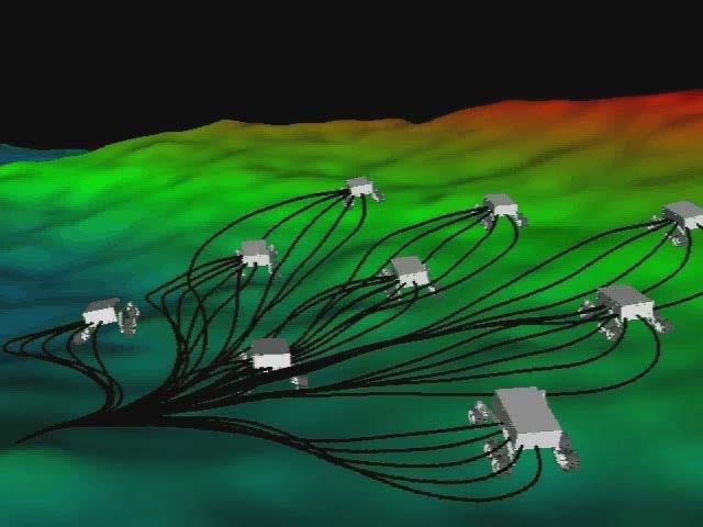
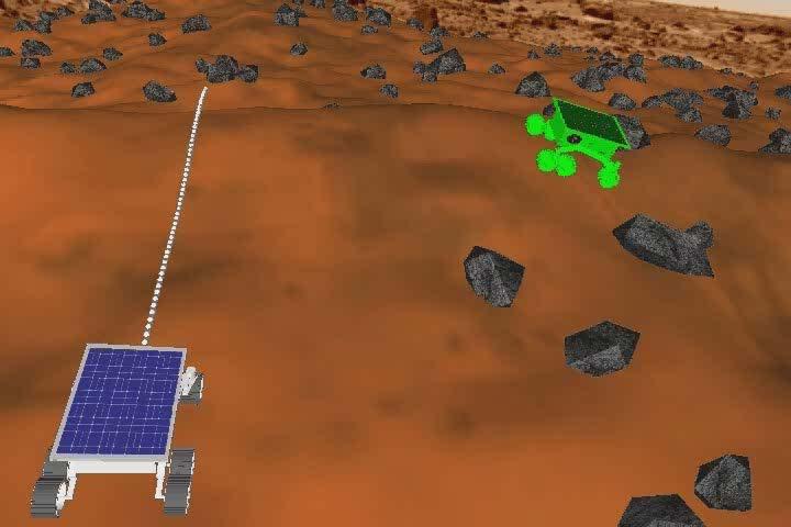
Multi-Robotic Systems
 CHAPTER 9 Multi-Robotic Systems The topic of multi-robotic systems is quite popular now. It is believed that such systems can have the following benefits: Improved performance ( winning by numbers ) Distributed
D(s) G(s) A control system design definition
 G(s) A control system design definition") R E Compensation D(s) U Plant G(s) Y Figure 7. A control system design definition x x x 2 x 2 U 2 s s 7 2 Y Figure 7.2 A block diagram representing Eq. (7.) in control form z U 2 s z Y 4 z 2 s z 2 3 Figure
R E Compensation D(s) U Plant G(s) Y Figure 7. A control system design definition x x x 2 x 2 U 2 s s 7 2 Y Figure 7.2 A block diagram representing Eq. (7.) in control form z U 2 s z Y 4 z 2 s z 2 3 Figure
Lecture Schedule Week Date Lecture (M: 2:05p-3:50, 50-N202)
") J = x θ τ = J T F 2018 School of Information Technology and Electrical Engineering at the University of Queensland Lecture Schedule Week Date Lecture (M: 2:05p-3:50, 50-N202) 1 23-Jul Introduction + Representing
J = x θ τ = J T F 2018 School of Information Technology and Electrical Engineering at the University of Queensland Lecture Schedule Week Date Lecture (M: 2:05p-3:50, 50-N202) 1 23-Jul Introduction + Representing
1 Kalman Filter Introduction
 1 Kalman Filter Introduction You should first read Chapter 1 of Stochastic models, estimation, and control: Volume 1 by Peter S. Maybec (available here). 1.1 Explanation of Equations (1-3) and (1-4) Equation
MCE693/793: Analysis and Control of Nonlinear Systems
 MCE693/793: Analysis and Control of Nonlinear Systems Input-Output and Input-State Linearization Zero Dynamics of Nonlinear Systems Hanz Richter Mechanical Engineering Department Cleveland State University
Robot Dynamics II: Trajectories & Motion
 Robot Dynamics II: Trajectories & Motion Are We There Yet? METR 4202: Advanced Control & Robotics Dr Surya Singh Lecture # 5 August 23, 2013 metr4202@itee.uq.edu.au http://itee.uq.edu.au/~metr4202/ 2013
ACM/CMS 107 Linear Analysis & Applications Fall 2016 Assignment 4: Linear ODEs and Control Theory Due: 5th December 2016
 ACM/CMS 17 Linear Analysis & Applications Fall 216 Assignment 4: Linear ODEs and Control Theory Due: 5th December 216 Introduction Systems of ordinary differential equations (ODEs) can be used to describe
Extremal Trajectories for Bounded Velocity Mobile Robots
 Extremal Trajectories for Bounded Velocity Mobile Robots Devin J. Balkcom and Matthew T. Mason Abstract Previous work [3, 6, 9, 8, 7, 1] has presented the time optimal trajectories for three classes of
Lecture 12. Upcoming labs: Final Exam on 12/21/2015 (Monday)10:30-12:30
10:30-12:30") 289 Upcoming labs: Lecture 12 Lab 20: Internal model control (finish up) Lab 22: Force or Torque control experiments [Integrative] (2-3 sessions) Final Exam on 12/21/2015 (Monday)10:30-12:30 Today: Recap
289 Upcoming labs: Lecture 12 Lab 20: Internal model control (finish up) Lab 22: Force or Torque control experiments [Integrative] (2-3 sessions) Final Exam on 12/21/2015 (Monday)10:30-12:30 Today: Recap
Chapter 3 Numerical Methods
 Chapter 3 Numerical Methods Part 2 3.2 Systems of Equations 3.3 Nonlinear and Constrained Optimization 1 Outline 3.2 Systems of Equations 3.3 Nonlinear and Constrained Optimization Summary 2 Outline 3.2
Relativistic Mechanics
 Physics 411 Lecture 9 Relativistic Mechanics Lecture 9 Physics 411 Classical Mechanics II September 17th, 2007 We have developed some tensor language to describe familiar physics we reviewed orbital motion
SIAM Conference on Applied Algebraic Geometry Daejeon, South Korea, Irina Kogan North Carolina State University. Supported in part by the
 SIAM Conference on Applied Algebraic Geometry Daejeon, South Korea, 2015 Irina Kogan North Carolina State University Supported in part by the 1 Based on: 1. J. M. Burdis, I. A. Kogan and H. Hong Object-image
Lecture 12. AO Control Theory
 Lecture 12 AO Control Theory Claire Max with many thanks to Don Gavel and Don Wiberg UC Santa Cruz February 18, 2016 Page 1 What are control systems? Control is the process of making a system variable
CBE507 LECTURE III Controller Design Using State-space Methods. Professor Dae Ryook Yang
 CBE507 LECTURE III Controller Design Using State-space Methods Professor Dae Ryook Yang Fall 2013 Dept. of Chemical and Biological Engineering Korea University Korea University III -1 Overview States What
Mobile Robotics, Mathematics, Models, and Methods
 Mobile Robotics, Mathematics, Models, and Methods Errata in Initial Revision Prepared by Professor Alonzo Kelly Rev 10, June 0, 015 Locations in the first column are given in several formats: 1 x,y,z means
Trajectory tracking & Path-following control
 Cooperative Control of Multiple Robotic Vehicles: Theory and Practice Trajectory tracking & Path-following control EECI Graduate School on Control Supélec, Feb. 21-25, 2011 A word about T Tracking and
Video 6.1 Vijay Kumar and Ani Hsieh
 Video 6.1 Vijay Kumar and Ani Hsieh Robo3x-1.6 1 In General Disturbance Input + - Input Controller + + System Output Robo3x-1.6 2 Learning Objectives for this Week State Space Notation Modeling in the
ELEC4631 s Lecture 2: Dynamic Control Systems 7 March Overview of dynamic control systems
 ELEC4631 s Lecture 2: Dynamic Control Systems 7 March 2011 Overview of dynamic control systems Goals of Controller design Autonomous dynamic systems Linear Multi-input multi-output (MIMO) systems Bat flight
Modeling and Analysis of Dynamic Systems
 Modeling and Analysis of Dynamic Systems by Dr. Guillaume Ducard Fall 2016 Institute for Dynamic Systems and Control ETH Zurich, Switzerland based on script from: Prof. Dr. Lino Guzzella 1/33 Outline 1
Here represents the impulse (or delta) function. is an diagonal matrix of intensities, and is an diagonal matrix of intensities.
 function. is an diagonal matrix of intensities, and is an diagonal matrix of intensities.") 19 KALMAN FILTER 19.1 Introduction In the previous section, we derived the linear quadratic regulator as an optimal solution for the fullstate feedback control problem. The inherent assumption was that
19 KALMAN FILTER 19.1 Introduction In the previous section, we derived the linear quadratic regulator as an optimal solution for the fullstate feedback control problem. The inherent assumption was that
AUTOMATIC CONTROL. Andrea M. Zanchettin, PhD Spring Semester, Introduction to Automatic Control & Linear systems (time domain)
") 1 AUTOMATIC CONTROL Andrea M. Zanchettin, PhD Spring Semester, 2018 Introduction to Automatic Control & Linear systems (time domain) 2 What is automatic control? From Wikipedia Control theory is an interdisciplinary
1 AUTOMATIC CONTROL Andrea M. Zanchettin, PhD Spring Semester, 2018 Introduction to Automatic Control & Linear systems (time domain) 2 What is automatic control? From Wikipedia Control theory is an interdisciplinary
Control Systems. State Estimation.
 State Estimation chibum@seoultech.ac.kr Outline Dominant pole design Symmetric root locus State estimation We are able to place the CLPs arbitrarily by feeding back all the states: u = Kx. But these may
13 Path Planning Cubic Path P 2 P 1. θ 2
 13 Path Planning Path planning includes three tasks: 1 Defining a geometric curve for the end-effector between two points. 2 Defining a rotational motion between two orientations. 3 Defining a time function
Linear State Feedback Controller Design
 Assignment For EE5101 - Linear Systems Sem I AY2010/2011 Linear State Feedback Controller Design Phang Swee King A0033585A Email: king@nus.edu.sg NGS/ECE Dept. Faculty of Engineering National University
Chap. 3. Controlled Systems, Controllability
 Chap. 3. Controlled Systems, Controllability 1. Controllability of Linear Systems 1.1. Kalman s Criterion Consider the linear system ẋ = Ax + Bu where x R n : state vector and u R m : input vector. A :
Control of Electromechanical Systems
 Control of Electromechanical Systems November 3, 27 Exercise Consider the feedback control scheme of the motor speed ω in Fig., where the torque actuation includes a time constant τ A =. s and a disturbance
Delay Coordinate Embedding
 Chapter 7 Delay Coordinate Embedding Up to this point, we have known our state space explicitly. But what if we do not know it? How can we then study the dynamics is phase space? A typical case is when
MEAM 520. More Velocity Kinematics
 MEAM 520 More Velocity Kinematics Katherine J. Kuchenbecker, Ph.D. General Robotics, Automation, Sensing, and Perception Lab (GRASP) MEAM Department, SEAS, University of Pennsylvania Lecture 12: October
NONLINEAR PATH CONTROL FOR A DIFFERENTIAL DRIVE MOBILE ROBOT
 NONLINEAR PATH CONTROL FOR A DIFFERENTIAL DRIVE MOBILE ROBOT Plamen PETROV Lubomir DIMITROV Technical University of Sofia Bulgaria Abstract. A nonlinear feedback path controller for a differential drive
Chapter 14: Vector Calculus
 Chapter 14: Vector Calculus Introduction to Vector Functions Section 14.1 Limits, Continuity, Vector Derivatives a. Limit of a Vector Function b. Limit Rules c. Component By Component Limits d. Continuity
Trajectory-tracking control of a planar 3-RRR parallel manipulator
 Trajectory-tracking control of a planar 3-RRR parallel manipulator Chaman Nasa and Sandipan Bandyopadhyay Department of Engineering Design Indian Institute of Technology Madras Chennai, India Abstract
Control Systems Design
 ELEC4410 Control Systems Design Lecture 18: State Feedback Tracking and State Estimation Julio H. Braslavsky julio@ee.newcastle.edu.au School of Electrical Engineering and Computer Science Lecture 18:
An Introduction to Control Systems
 An Introduction to Control Systems Signals and Systems: 3C1 Control Systems Handout 1 Dr. David Corrigan Electronic and Electrical Engineering corrigad@tcd.ie November 21, 2012 Recall the concept of a
Lecture 9. Introduction to Kalman Filtering. Linear Quadratic Gaussian Control (LQG) G. Hovland 2004
 G. Hovland 2004") MER42 Advanced Control Lecture 9 Introduction to Kalman Filtering Linear Quadratic Gaussian Control (LQG) G. Hovland 24 Announcement No tutorials on hursday mornings 8-9am I will be present in all practical
MER42 Advanced Control Lecture 9 Introduction to Kalman Filtering Linear Quadratic Gaussian Control (LQG) G. Hovland 24 Announcement No tutorials on hursday mornings 8-9am I will be present in all practical
Orbital Motion in Schwarzschild Geometry
 Physics 4 Lecture 29 Orbital Motion in Schwarzschild Geometry Lecture 29 Physics 4 Classical Mechanics II November 9th, 2007 We have seen, through the study of the weak field solutions of Einstein s equation
An introduction to Mathematical Theory of Control
 An introduction to Mathematical Theory of Control Vasile Staicu University of Aveiro UNICA, May 2018 Vasile Staicu (University of Aveiro) An introduction to Mathematical Theory of Control UNICA, May 2018
(Refer Slide Time: 00:32)
") Nonlinear Dynamical Systems Prof. Madhu. N. Belur and Prof. Harish. K. Pillai Department of Electrical Engineering Indian Institute of Technology, Bombay Lecture - 12 Scilab simulation of Lotka Volterra
Nonlinear Dynamical Systems Prof. Madhu. N. Belur and Prof. Harish. K. Pillai Department of Electrical Engineering Indian Institute of Technology, Bombay Lecture - 12 Scilab simulation of Lotka Volterra
Game Physics. Game and Media Technology Master Program - Utrecht University. Dr. Nicolas Pronost
 Game and Media Technology Master Program - Utrecht University Dr. Nicolas Pronost Essential physics for game developers Introduction The primary issues Let s move virtual objects Kinematics: description
Control Systems Design, SC4026. SC4026 Fall 2009, dr. A. Abate, DCSC, TU Delft
 Control Systems Design, SC4026 SC4026 Fall 2009, dr. A. Abate, DCSC, TU Delft Lecture 4 Controllability (a.k.a. Reachability) vs Observability Algebraic Tests (Kalman rank condition & Hautus test) A few
Figure 1: Functions Viewed Optically. Math 425 Lecture 4. The Chain Rule
 Figure 1: Functions Viewed Optically Math 425 Lecture 4 The Chain Rule The Chain Rule in the One Variable Case We explain the chain rule in the one variable case. To do this we view a function f as a impossible
Subject: Optimal Control Assignment-1 (Related to Lecture notes 1-10)
") Subject: Optimal Control Assignment- (Related to Lecture notes -). Design a oil mug, shown in fig., to hold as much oil possible. The height and radius of the mug should not be more than 6cm. The mug must
Subject: Optimal Control Assignment- (Related to Lecture notes -). Design a oil mug, shown in fig., to hold as much oil possible. The height and radius of the mug should not be more than 6cm. The mug must
r CM = ir im i i m i m i v i (2) P = i
 P = i") Physics 121 Test 3 study guide Thisisintendedtobeastudyguideforyourthirdtest, whichcoverschapters 9, 10, 12, and 13. Note that chapter 10 was also covered in test 2 without section 10.7 (elastic collisions),
Physics 121 Test 3 study guide Thisisintendedtobeastudyguideforyourthirdtest, whichcoverschapters 9, 10, 12, and 13. Note that chapter 10 was also covered in test 2 without section 10.7 (elastic collisions),
Good Problems. Math 641
 Math 641 Good Problems Questions get two ratings: A number which is relevance to the course material, a measure of how much I expect you to be prepared to do such a problem on the exam. 3 means of course
Robotics & Automation. Lecture 25. Dynamics of Constrained Systems, Dynamic Control. John T. Wen. April 26, 2007
 Robotics & Automation Lecture 25 Dynamics of Constrained Systems, Dynamic Control John T. Wen April 26, 2007 Last Time Order N Forward Dynamics (3-sweep algorithm) Factorization perspective: causal-anticausal
L03. PROBABILITY REVIEW II COVARIANCE PROJECTION. NA568 Mobile Robotics: Methods & Algorithms
 L03. PROBABILITY REVIEW II COVARIANCE PROJECTION NA568 Mobile Robotics: Methods & Algorithms Today s Agenda State Representation and Uncertainty Multivariate Gaussian Covariance Projection Probabilistic
Lab I. 2D Motion. 1 Introduction. 2 Theory. 2.1 scalars and vectors LAB I. 2D MOTION 15
 LAB I. 2D MOTION 15 Lab I 2D Motion 1 Introduction In this lab we will examine simple two-dimensional motion without acceleration. Motion in two dimensions can often be broken up into two separate one-dimensional
Introduction to Control (034040) lecture no. 2
 lecture no. 2") Introduction to Control (034040) lecture no. 2 Leonid Mirkin Faculty of Mechanical Engineering Technion IIT Setup: Abstract control problem to begin with y P(s) u where P is a plant u is a control signal
Introduction to Control (034040) lecture no. 2 Leonid Mirkin Faculty of Mechanical Engineering Technion IIT Setup: Abstract control problem to begin with y P(s) u where P is a plant u is a control signal
Trajectory planning and feedforward design for electromechanical motion systems version 2
 2 Trajectory planning and feedforward design for electromechanical motion systems version 2 Report nr. DCT 2003-8 Paul Lambrechts Email: P.F.Lambrechts@tue.nl April, 2003 Abstract This report considers
Positioning Servo Design Example
 Positioning Servo Design Example 1 Goal. The goal in this design example is to design a control system that will be used in a pick-and-place robot to move the link of a robot between two positions. Usually
Laboratory Exercise 1 DC servo
 Laboratory Exercise DC servo Per-Olof Källén ø 0,8 POWER SAT. OVL.RESET POS.RESET Moment Reference ø 0,5 ø 0,5 ø 0,5 ø 0,65 ø 0,65 Int ø 0,8 ø 0,8 Σ k Js + d ø 0,8 s ø 0 8 Off Off ø 0,8 Ext. Int. + x0,
Module 07 Controllability and Controller Design of Dynamical LTI Systems
 Module 07 Controllability and Controller Design of Dynamical LTI Systems Ahmad F. Taha EE 5143: Linear Systems and Control Email: ahmad.taha@utsa.edu Webpage: http://engineering.utsa.edu/ataha October
Lab I. 2D Motion. 1 Introduction. 2 Theory. 2.1 scalars and vectors LAB I. 2D MOTION 15
 LAB I. 2D MOTION 15 Lab I 2D Motion 1 Introduction In this lab we will examine simple two-dimensional motion without acceleration. Motion in two dimensions can often be broken up into two separate one-dimensional
CONTROL OF THE NONHOLONOMIC INTEGRATOR
 June 6, 25 CONTROL OF THE NONHOLONOMIC INTEGRATOR R. N. Banavar (Work done with V. Sankaranarayanan) Systems & Control Engg. Indian Institute of Technology, Bombay Mumbai -INDIA. banavar@iitb.ac.in Outline
MATH4406 (Control Theory) Unit 1: Introduction Prepared by Yoni Nazarathy, July 21, 2012
 Unit 1: Introduction Prepared by Yoni Nazarathy, July 21, 2012") MATH4406 (Control Theory) Unit 1: Introduction Prepared by Yoni Nazarathy, July 21, 2012 Unit Outline Introduction to the course: Course goals, assessment, etc... What is Control Theory A bit of jargon,
MATH4406 (Control Theory) Unit 1: Introduction Prepared by Yoni Nazarathy, July 21, 2012 Unit Outline Introduction to the course: Course goals, assessment, etc... What is Control Theory A bit of jargon,
Fall 線性系統 Linear Systems. Chapter 08 State Feedback & State Estimators (SISO) Feng-Li Lian. NTU-EE Sep07 Jan08
 Feng-Li Lian. NTU-EE Sep07 Jan08") Fall 2007 線性系統 Linear Systems Chapter 08 State Feedback & State Estimators (SISO) Feng-Li Lian NTU-EE Sep07 Jan08 Materials used in these lecture notes are adopted from Linear System Theory & Design, 3rd.
Fall 2007 線性系統 Linear Systems Chapter 08 State Feedback & State Estimators (SISO) Feng-Li Lian NTU-EE Sep07 Jan08 Materials used in these lecture notes are adopted from Linear System Theory & Design, 3rd.
Nonlinear Observers. Jaime A. Moreno. Eléctrica y Computación Instituto de Ingeniería Universidad Nacional Autónoma de México
 Nonlinear Observers Jaime A. Moreno JMorenoP@ii.unam.mx Eléctrica y Computación Instituto de Ingeniería Universidad Nacional Autónoma de México XVI Congreso Latinoamericano de Control Automático October
Robotics. Control Theory. Marc Toussaint U Stuttgart
 Robotics Control Theory Topics in control theory, optimal control, HJB equation, infinite horizon case, Linear-Quadratic optimal control, Riccati equations (differential, algebraic, discrete-time), controllability,
II. Unit Speed Curves
 The Geometry of Curves, Part I Rob Donnelly From Murray State University s Calculus III, Fall 2001 note: This material supplements Sections 13.3 and 13.4 of the text Calculus with Early Transcendentals,
Video 5.1 Vijay Kumar and Ani Hsieh
 Video 5.1 Vijay Kumar and Ani Hsieh Robo3x-1.1 1 The Purpose of Control Input/Stimulus/ Disturbance System or Plant Output/ Response Understand the Black Box Evaluate the Performance Change the Behavior
Tangent spaces, normals and extrema
 Chapter 3 Tangent spaces, normals and extrema If S is a surface in 3-space, with a point a S where S looks smooth, i.e., without any fold or cusp or self-crossing, we can intuitively define the tangent
Control of Mobile Robots Prof. Luca Bascetta
 Control of Mobile Robots Prof. Luca Bascetta EXERCISE 1 1. Consider a wheel rolling without slipping on the horizontal plane, keeping the sagittal plane in the vertical direction. Write the expression
Mobile Manipulation: Force Control
 8803 - Mobile Manipulation: Force Control Mike Stilman Robotics & Intelligent Machines @ GT Georgia Institute of Technology Atlanta, GA 30332-0760 February 19, 2008 1 Force Control Strategies Logic Branching
AC&ST AUTOMATIC CONTROL AND SYSTEM THEORY SYSTEMS AND MODELS. Claudio Melchiorri
 C. Melchiorri (DEI) Automatic Control & System Theory 1 AUTOMATIC CONTROL AND SYSTEM THEORY SYSTEMS AND MODELS Claudio Melchiorri Dipartimento di Ingegneria dell Energia Elettrica e dell Informazione (DEI)
Control System Design
 ELEC ENG 4CL4: Control System Design Notes for Lecture #36 Dr. Ian C. Bruce Room: CRL-229 Phone ext.: 26984 Email: ibruce@mail.ece.mcmaster.ca Friday, April 4, 2003 3. Cascade Control Next we turn to an
ECE557 Systems Control
 ECE557 Systems Control Bruce Francis Course notes, Version.0, September 008 Preface This is the second Engineering Science course on control. It assumes ECE56 as a prerequisite. If you didn t take ECE56,
Control Systems Design, SC4026. SC4026 Fall 2010, dr. A. Abate, DCSC, TU Delft
 Control Systems Design, SC4026 SC4026 Fall 2010, dr. A. Abate, DCSC, TU Delft Lecture 4 Controllability (a.k.a. Reachability) and Observability Algebraic Tests (Kalman rank condition & Hautus test) A few
Analysis of Critical Speed Yaw Scuffs Using Spiral Curves
 Analysis of Critical Speed Yaw Scuffs Using Spiral Curves Jeremy Daily Department of Mechanical Engineering University of Tulsa PAPER #2012-01-0606 Presentation Overview Review of Critical Speed Yaw Analysis
CHAPTER 1. Introduction
 CHAPTER 1 Introduction Linear geometric control theory was initiated in the beginning of the 1970 s, see for example, [1, 7]. A good summary of the subject is the book by Wonham [17]. The term geometric
Controlling the Apparent Inertia of Passive Human- Interactive Robots
 Controlling the Apparent Inertia of Passive Human- Interactive Robots Tom Worsnopp Michael Peshkin J. Edward Colgate Kevin Lynch Laboratory for Intelligent Mechanical Systems: Mechanical Engineering Department
Non-holonomic constraint example A unicycle
 Non-holonomic constraint example A unicycle A unicycle (in gray) moves on a plane; its motion is given by three coordinates: position x, y and orientation θ. The instantaneous velocity v = [ ẋ ẏ ] is along
Mobile Robotics 1. A Compact Course on Linear Algebra. Giorgio Grisetti
 Mobile Robotics 1 A Compact Course on Linear Algebra Giorgio Grisetti SA-1 Vectors Arrays of numbers They represent a point in a n dimensional space 2 Vectors: Scalar Product Scalar-Vector Product Changes
10/8/2015. Control Design. Pole-placement by state-space methods. Process to be controlled. State controller
 Pole-placement by state-space methods Control Design To be considered in controller design * Compensate the effect of load disturbances * Reduce the effect of measurement noise * Setpoint following (target
Where we ve been, where we are, and where we are going next.
 6.302.0x, January 2016 Notes Set 2 1 MASSACHVSETTS INSTITVTE OF TECHNOLOGY Department of Electrical Engineering and Computer Science 6.302.0x Introduction to Feedback System Design January 2016 Notes Set
Robust Control of Cooperative Underactuated Manipulators
 Robust Control of Cooperative Underactuated Manipulators Marcel Bergerman * Yangsheng Xu +,** Yun-Hui Liu ** * Automation Institute Informatics Technology Center Campinas SP Brazil + The Robotics Institute
Active Nonlinear Observers for Mobile Systems
 Active Nonlinear Observers for Mobile Systems Simon Cedervall and Xiaoming Hu Optimization and Systems Theory Royal Institute of Technology SE 00 44 Stockholm, Sweden Abstract For nonlinear systems in
Lecture 9 Nonlinear Control Design
 Lecture 9 Nonlinear Control Design Exact-linearization Lyapunov-based design Lab 2 Adaptive control Sliding modes control Literature: [Khalil, ch.s 13, 14.1,14.2] and [Glad-Ljung,ch.17] Course Outline
Solution of Linear Equations
 Solution of Linear Equations (Com S 477/577 Notes) Yan-Bin Jia Sep 7, 07 We have discussed general methods for solving arbitrary equations, and looked at the special class of polynomial equations A subclass
Control Systems I. Lecture 2: Modeling. Suggested Readings: Åström & Murray Ch. 2-3, Guzzella Ch Emilio Frazzoli
 Control Systems I Lecture 2: Modeling Suggested Readings: Åström & Murray Ch. 2-3, Guzzella Ch. 2-3 Emilio Frazzoli Institute for Dynamic Systems and Control D-MAVT ETH Zürich September 29, 2017 E. Frazzoli
Definition 5.1. A vector field v on a manifold M is map M T M such that for all x M, v(x) T x M.
 T x M.") 5 Vector fields Last updated: March 12, 2012. 5.1 Definition and general properties We first need to define what a vector field is. Definition 5.1. A vector field v on a manifold M is map M T M such that
5 Vector fields Last updated: March 12, 2012. 5.1 Definition and general properties We first need to define what a vector field is. Definition 5.1. A vector field v on a manifold M is map M T M such that
Position and orientation of rigid bodies
 Robotics 1 Position and orientation of rigid bodies Prof. Alessandro De Luca Robotics 1 1 Position and orientation right-handed orthogonal Reference Frames RF A A p AB B RF B rigid body position: A p AB
Extremal Trajectories for Bounded Velocity Differential Drive Robots
 Extremal Trajectories for Bounded Velocity Differential Drive Robots Devin J. Balkcom Matthew T. Mason Robotics Institute and Computer Science Department Carnegie Mellon University Pittsburgh PA 523 Abstract
10 Transfer Matrix Models
 MIT EECS 6.241 (FALL 26) LECTURE NOTES BY A. MEGRETSKI 1 Transfer Matrix Models So far, transfer matrices were introduced for finite order state space LTI models, in which case they serve as an important
Case Study: The Pelican Prototype Robot
 5 Case Study: The Pelican Prototype Robot The purpose of this chapter is twofold: first, to present in detail the model of the experimental robot arm of the Robotics lab. from the CICESE Research Center,
Department of Aerospace Engineering and Mechanics University of Minnesota Written Preliminary Examination: Control Systems Friday, April 9, 2010
 Department of Aerospace Engineering and Mechanics University of Minnesota Written Preliminary Examination: Control Systems Friday, April 9, 2010 Problem 1: Control of Short Period Dynamics Consider the
Disturbance Decoupling and Unknown-Input Observation Problems
 Disturbance Decoupling and Unknown-Input Observation Problems Lorenzo Ntogramatzidis Curtin University of Technology, Australia MTNS - July 5-9, 2010 L. Ntogramatzidis (Curtin University) MTNS - July 5-9,
Nonlinear dynamics & chaos BECS
 Nonlinear dynamics & chaos BECS-114.7151 Phase portraits Focus: nonlinear systems in two dimensions General form of a vector field on the phase plane: Vector notation: Phase portraits Solution x(t) describes
Control System Design
 ELEC ENG 4CL4: Control System Design Notes for Lecture #24 Wednesday, March 10, 2004 Dr. Ian C. Bruce Room: CRL-229 Phone ext.: 26984 Email: ibruce@mail.ece.mcmaster.ca Remedies We next turn to the question