Minimal Element Interpolation in Functions of High-Dimension

Transcription

1 Minimal Element Interpolation in Functions of High-Dimension J. D. Jakeman, A. Narayan, D. Xiu Department of Mathematics Purdue University West Lafayette, Indiana

2 Random Model as a function We can consider the stochastic model as a deterministic function dependent on the variables u(ξ) }{{} Observables = M(ξ) }{{} Model

3 Adaptive Approximation Methods Figure: Local hierarchical adaptivity Figure: Three possible refinement of a element E k. The top element being refined will produce decomposition (a) if, decomposition (b) or decomposition (c)

4 Domain Decomposition Use discontinuity detection to decompose input space into regions of high-regularity Figure: Hyper-cube vs arbitrary shaped element decomposition

5 Polynomial Annihilation Discontinuity Detection We seek an approximation to [f ](x) that converges rapidly to zero away from the jump discontinuities. Consider a piecewise continuous function f (x) : [ 1, 1] R known only on the set of discrete points S = {x 1, x 2,..., x Q (1)} [ 1, 1]. The local jump function is defined as [f ](x) = f ( x +) f ( x ) { 0, if x ξ, = [f ] (ξ), if x = ξ. If f is continuous at x, [f ](x) = 0; if x is a point of discontinuity of f, then [f ](x) is equal to the jump value there.

6 Polynomial Annihilation Discontinuity Detection For a given positive integer m < Q (1) 1, we choose a local stencil S x = {x j x j S} = {x 0,..., x m } We approximate the jump function by L m f (x) = 1 q m (x) x j S x c j (x)f (x j ), c j (x) are chosen to annihilate polynomials of degree up to m 1 and are determined by solving the linear system c j (x)p i (x j ) = p (m) i (x), i = 0,, m. x j S x p (m) i (x) denotes the mth derivative of p i (x).

7 Discontinuity Detection - Minmod Limiter MM(L m f (x)) = Given M = {1, 2,..., µ} { minm M L m f (x), if L m f (x) > 0, m M, max m M L m f (x), if L m f (x) < 0, m M, 0, otherwise,

8 Polynomial Annihilation Discontinuity Detection Given a maximum separation h(x) defined by h(x) = max{ x i x i 1 : x i 1, x i S x }, then L m f (x) satisfies the following property: MM(L M f (x)) = { [f ](ξ) + O(h(x)), if xj 1 ξ, x x j, O(h min(mx,k) (x)), if f C k (I x ), k > 0. M x = max{m M #S x = m + 1, (S x I x ) J = }

9 High-Dimensional Discontinuity Detection Step I Step II Step III Step IV Step V Figure: Five steps of the discontinuity detection algorithm applied to a 1D domain

10 Discontinuity Tracking - Illustrative Example Example Consider the following function { 1, d f (x) = i=1 x i 2 < r 2 and x 1 < 0 x 1, otherwise.

11 Discontinuity Tracking

12 Discontinuity Tracking Consider the following function: { 1, k f (x) = i=1 x i 2 < r 2, k d 0, otherwise which has a simple analytic expression of the distance function to the nearest discontinuity D f (x) = ( k ) 12. r xi 2 i=1

13 Discontinuity Tracking

14 High-Dimensional Discontinuity Detection Anova decomposition d d u(ξ 1,..., ξ d ) = u 0 + u(ξ i ) + u(ξ i, ξ j ) + + u(ξ 1,..., ξ d ) i=1 i,j=1 Perform smart initial sampling to identify dimensions that lie on discontinuity manifold Limit dimensions considered to those on the manifold

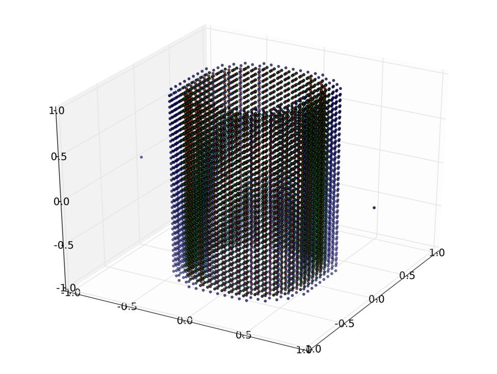
15 High-Dimensional Discontinuity Detection

16 Estimating Distance Functions

17 Numerical Convergence f (x) = j P 1, k i=1 x i 2 < r 2, k d 0, otherwise d N ɛ max Table: ɛ max error in approximated distance function as dimensionality of input space increases. Figure: Convergence with δ

18 Interpolation on Arbitrary Nodes The goal is to construct a practical algorithm for polynomial interpolation on arbitrary nodal sets. Given an unpredictable set of interpolation nodes How can we choose an appropriate basis? How do we avoid ill-conditioning? (x 4, y 4 ) (x 2, y 2 ) (x 1, y 1 ) (x 3, y 3 ) Basis candidates: 1 x y x 2 xy y 2

19 Motivation The goal: find p N = M m=0 c mφ m satisfying p N (x n ) = f n The restatement: find a polynomial space Π X that is correct for the nodal set X Inputs Nodes x Basis construction Form matrix A Solve Ac = f Data f The method computes a subspace of polynomials of the same dimension as the number of nodes.

20 Minimal Element Interpolation Minimal Element Interpolation Method Use discontinuity detection to decompose the input domain into disjoint regions of high regularity Apply least interpolation on each element How do we chose interpolation nodes? Reuse the points constructed when detecting the discontinuities

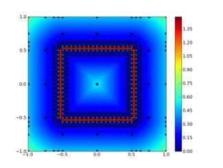
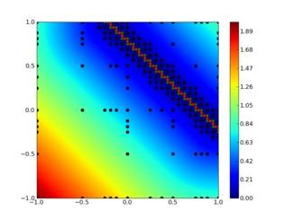
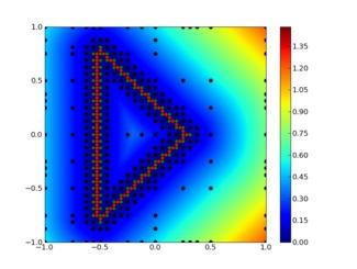
21 Figure: Minimal element approximation of the square circular and triangular manifold discontinuities. Top contour plot of approximation. Bottom contour plot of true function and points used to construct approximation.

22 Table: Square manifold d = m = 2 (490 points) Interior Exterior L 1 error L 2 error L error L 1 error L 2 error L error N = e e e+00 N = e e e+00 N = e e e-01 N = e e e+02 N = e e e-01 N = e e e+00 N = e e e-02 N = e e e-01 N = e e e-03 N = e e e-02

23 Table: Spherical manifold d = m = 2 (574 points) Interior Exterior L 1 error L 2 error L error L 1 error L 2 error L error N = e e e+00 N = e e e+00 N = e e e-02 N = e e e+00 N = e e e-03 N = e e e+01 N = e e e-04 N = e e e+00 N = e e e-04 N = e e e-01 Table: Triangle manifold d = m = 2 (518 points) Interior Exterior L 1 error L 2 error L error L 1 error L 2 error L error N = e e e+00 N = e e e+00 N = e e e+00 N = e e e+01 N = e e e-01 N = e e e+01 N = e e e-01 N = e e e+01 N = e e e-02 N = e e e+01

24 Figure: Minimal element approximation of the circular and triangular manifold discontinuities

25 Table: L 2 error in the interior ε int and exterior ε ext domains. Minimal Element Adaptive Sparse Grid Function N M ε int ε ext N ε int ε ext Sphere e e e e-04 Square e e e e-03 Triangle e e e e-03 Table: Error in the interior defined by the 3D mainfold of spherical discontinuity in 10 dimensions (3495 points) L 1 error L 2 error L error N = e e e-01 N = e e e-02 N = e e e-03 N = e e e-04

26 Conclusions Strengths Independent of any specific shape of discontinuities Discontinuity detection possesses a fast rate of convergence to zero away from the discontinuities The discontinuity detection method scales linearly with total dimension High order convergence in disjoint elements Weaknesses If the dimensionality/surface area of the discontinuity manifold is large representation of the manifold will become infeasible Poor accuracy in regions where not many nodes exist Future Work Extend to discontinuities in derivatives Determine how to select points in dimensions which do not lie on the discontinuity manifold and in regions where function evaluations used by the discontinuity algorithm are sparse