Irrigation Conveyance & Control: Flow Measurement & Structure Design

Transcription

1 BIE 5300/6300 Fall Semester 2004 Irrigation Conveyance & Control: Flow Measurement & Structure Design Lecture Notes Biological & Irrigation Engineering Department Utah State University, Logan, Utah

2 Gary P. Merkley ii BIE 5300/6300 Lectures

3 Preface These lecture notes were prepared by Gary P. Merkley of the Biological & Irrigation Engineering Department at USU for use in the BIE 5300/6300 courses. The material contained in these lecture notes is the intellectual property right of G.P. Merkley, except where otherwise stated. Many thanks are extended to USU engineering students, past and present, whose numerous suggestions and corrections have been incorporated into these lecture notes. Copyright Notice This material has been duplicated by special permission of the copyright holder. It is not to be duplicated or used for purposes other than learning resource support for Utah State University. Any violation of this agreement is punishable under existing copyright laws. Copyright 2000, 2001, 2002, 2003, 2004 BIE 5300/6300 Lectures iii Gary P. Merkley

4 Gary P. Merkley iv BIE 5300/6300 Lectures

5 C o n t e n t s Page 1 Course Introduction Flumes for Open-Channel Flow Measurement Current Metering in Open Channels Current Metering in Open Channels Field Exercise #1 for Open-Channel Flow Measurement Field Exercise #2 for Open-Channel Flow Measurement Weirs for Flow Measurement Weirs for Flow Measurement Broad Crested Weirs Broad Crested Weirs Calibration of Canal Gates Calibration of Canal Gates Flow Measurement in Pipes Flow Measurement in Pipes Canal Design Basics Channel Cross Sections Design of Earthen Canals Sample Earthen Canal Designs Canal Linings Inverted Siphons Culvert Design & Analysis Sample Culvert Designs Culvert Hydraulic Behavior Flumes & Channel Transitions Design Example for a Channel Transition Energy Dissipation Structures Protective Structures Safety Considerations These lecture notes are formatting for printing on both sides of the page, with oddnumbered pages on the front. Each lecture begins on an odd-numbered page, so some even-numbered pages are blank. BIE 5300/6300 Lectures v Gary P. Merkley

6 Gary P. Merkley vi BIE 5300/6300 Lectures

7 Units, Constants and Conversions g/oz gpm/lps (= 60/3.785) gallons/ft gpm/cfs (= 7.481*60) litres/gallon 6.89 kpa/psi 1 cb = 1 kpa 10 mb/kpa, or 100 kpa/bar ft/psi, or 9.81 kpa/m (head of water) 14.7 psi = kpa = m (head of water) = 1,013 mbar = 1 atm 62.4 lbs/ft 3, or 1000 kg/m 3 (max density of pure water at 4 C) kpa/mmhg 1 ppm 1 mg/liter (usually) 1 mmho/cm = 1 ds/m = 550 to 800 mg/liter kw/hp 1 langley = 1 cal/cm MJ/m 2 per cal/cm m/ft km/mile acre/ha 43,560 ft 2 /acre 1,233 m 3 /acre-ft degrees/radian π e ºC = (ºF 32)/1.8 ºF = 1.8(ºC) + 32 Ratio of weight to mass at sea level and 45 latitude: g = m/s 2 BIE 5300/6300 Lectures vii Gary P. Merkley

8 Gary P. Merkley viii BIE 5300/6300 Lectures

9 Lecture 1 Course Introduction I. Textbook and Other Materials What is never measured is never managed Rep. Stephen Urquhart (2003) The main references are Design of Small Canal Structures, USBR; and Water Measurement Manual, USBR. At least one copy of each will be on reserve in the library. Some material will also be referred to from Irrigation Fundamentals, by Hargreaves & Merkley, as well as from other books and sources BIE 5300/6300 lecture notes by G.P. Merkley are required II. Homework All work must be organized and neat There will be some computer programming and or spreadsheet exercises Submitting work late:10% reduction per day, starting after class III. Tests One mid-term exam Final exam is not comprehensive IV. Subject Areas Flow measurement Open channels Full pipe flow Design of conveyance infrastructure Canals, flumes, chutes Canal linings Siphons Culverts Energy dissipation structures V. Why Measure Water? Flow measurement is a key element in: 1. Water Management. Without knowing flow rates it is usually difficult to quantify deliveries to water users, and in this case the evaluation of water management practices is only vague 2. Water Quality Analysis. This relates to concentrations, rate of movement, direction of movement, and dispersion of contaminants, and other issues BIE 5300/6300 Lectures 1 Gary P. Merkley

10 3. Water Rights and Water Law. This includes volumetric delivery allotments, groundwater pumping, and excess water (e.g. irrigation runoff), among others Good quality, fresh water, is becoming more and more scarce as people exploit water resources more aggressively, and as the world population increases This increases the importance of water measurement It is unlikely that the regional and global situations on water availability and water quality will improve in the foreseeable future When a resource is measured, it is implied that it has significant value; when not measured, the implication is of little or no value Nilometer, Cairo, Egypt VI. Some Fundamental Flow Measurement Concepts Most flow measurement devices and techniques are based on the measurement of head (depth or pressure) or velocity One exception to this is the salt dilution method (described below) Here, the term flow rate refers to volumetric rate, or volume per unit time Thus, we apply mathematical relationships between head and discharge, or take products of velocity and cross-sectional area Strictly speaking, all open-channel and most pipe flow measurement techniques cause head loss The inability to make accurate measurements is not necessarily because of instrumentation deficiencies, but is a fundamental property of the physical world you cannot measure something without changing it (paraphrased) W.K. Heisenberg ( ) However, some methods incur negligible losses (e.g. ultrasonic) It is usually desirable to have only a small head loss because this loss typically translates into an increased upstream flow depth in subcritical open-channel flow In open-channel flow measurement, devices can operate under free flow and submerged flow regimes In free flow, we are concerned with the upstream head because critical flow occurs in the vicinity of the flow measurement device. As long as this is true, changes in downstream depth will not affect discharge at that location. In submerged flow, we are concerned with a head differential across the flow measurement device. In this class, the terms flow rate and discharge will be used interchangeably. Gary P. Merkley 2 BIE 5300/6300 Lectures

11 VII. Flow Measurement Accuracy Perhaps the most accurate method for measuring flow rate is by timing the filling of a container of known volume However, this is often not practical for large flow rates Typical flow measurement accuracies are from ±2% to ±20% of the true discharge, but this range can be much greater Measurements of head, velocity, and area are subject to errors for a variety of reasons: 1. Approach Conditions High approach velocity Approach velocity not perpendicular to measurement device 2. Turbulence and Eddies Rough water surface Swirling flow near or at measurement location 3. Equipment Problems Staff gauges, current meters, floats, etc., in disrepair Shifting calibrations on pressure transducers and other meters Poor installation (non-horizontal crest, wrong dimensions, etc.) 4. Measurement Location Local measurements (uniform flow assumption?) Stream gauging stations (need steady flow) 5. Human Errors Misreading water levels, etc. Misuse of equipment, or improper application of equipment VIII. Simple Flow Measurement Methods The following are considered to be special methods, because they are mostly simple and approximate, and because they are not usually the preferred methods for flow measurement in open channels BIE 5300/6300 Lectures 3 Gary P. Merkley

12 Preferred methods are through the use of calibrated structures (weirs, flumes, orifices, and others), and current metering 1. Measurement by Observation In this method one must rely on experience to estimate the discharge in an open channel, simply by observing the flow in the channel and mentally comparing it to similar channels from which the flow rate was measured and known This method is usually not very accurate, especially for large flows, but some very experienced hydrographers can (with some luck) arrive at a close estimate 2. Measurement by Floats The average flow velocity in an open channel can be estimated by measuring the speed of a floating object on the surface of the water This can be done by marking uniform distances along the channel and using a watch to measure the elapsed time from a starting location to respective downstream locations However, in practice, usually only a single distance (say 10 m) is used float water surface 10 m It is a good idea to have more than one measurement point so that the velocity can be averaged over a reach, and to lessen the chance of an error Then, a graph can be made of float travel distance versus time, with the slope equal to the surface velocity of the water Select a location in which the channel is fairly straight, not much change in cross-section, smooth water surface, and no abrupt changes in bed elevation or longitudinal slope Note that wind can affect the velocity of the float, changing the relationship between surface velocity and average flow velocity Gary P. Merkley 4 BIE 5300/6300 Lectures

13 Care should be taken to obtain measurements with the float moving near the center of the surface width of flow, not bumping into the channel sides, and not sinking The float speed will be higher than the average flow velocity in the channel, unless perhaps the float travels near one of the channel banks or is obstructed by vegetation You can estimate the average velocity in the channel by reducing the float speed by some fraction The following table is from the U.S. Bureau of Reclamation It gives coefficients to multiply by the measured float velocity, as a function of average depth, to obtain the approximate average flow velocity in the channel Average Depth (ft) (m) Coefficient >20 > To obtain average depth, divide the cross-sectional area by the top width of the water surface (do not use an area-weighted average of subsection depths) The coefficients in the above table only give approximate results; you can typically expect errors of 10 to 20% in the flow rate What happens to the above coefficient values when the average water depth is below 1 ft (or 0.3 m)? Some hydrographers have used partially submerged wooden sticks which are designed to approximate the mean flow velocity, precluding the need for coefficients as in the above table One end of the stick is weighted so that is sinks further The stick will give the correct velocity only for a small range of water depths The float method is not precise because the relationship between float speed and true average flow velocity is not well known in general Other methods should be used if an accurate measurement is desired BIE 5300/6300 Lectures 5 Gary P. Merkley

14 Sample calculation: The float method is applied in a rectangular channel with a base width of 0.94 m and a uniform water depth of 0.45 m. Ten float travel times are recorded over a distance of 5.49 m (18 ft), with calculated surface velocities: Trial Time (s) V (m/s) Avg: Alternatively, the average surface velocity can be taken as 5.49/7.02 = m/s, which is very close to the average velocity of m/s from the above table (as is usually the case). The surface velocity coefficient can be taken as 0.67, interpolating in the previous table of USBR data, and the cross-sectional area of the channel is (0.45)( 0.94) = 0.42 m 2. Then, the estimated flow rate is: (0.67)(0.783 m/s)(0.42 m 2 ) = 0.22 m 3 /s 3. Dye Method The dye method, or color-velocity method, can be used to measure the flow velocity, similar to the float method However, in this method a slug of dye is injected into the stream, and the time for the slug of dye to reach a downstream location is measured This time can be taken as the average of the time for the first portion of the dye to reach the downstream location, and the time for the last portion of the dye to reach that location (the dye will disperse and elongate as it moves downstream). The test section should not be too long, otherwise the dye will have dispersed too much and it is difficult to visually detect the color differential in the water Usually, it is appropriate to use a test section of approximately 3 m Dyes used in this type of measurement should be nontoxic so as not to pollute the water Food coloring can be used, as can other colored chemicals, such as flouricine Gary P. Merkley 6 BIE 5300/6300 Lectures

15 4. Salt Dilution In this method, an aqueous solution of known salt concentration, C 1, is poured into the stream at a constant rate, q The completely mixed solution is measured at a downstream location, providing the concentration C 2 The downstream location should be at least 5 m (perhaps up to 10 or 15 m) from the point of injection, otherwise incomplete mixing may result in large errors; that is, you might measure a highly-concentrated slug of water, or you might miss the slug altogether, if you try to measure too close to the point of injection After measuring the existing salt concentration in the flow (without adding the concentrated solution), C 0, the stream discharge, Q, can be calculated as, [ ] [ ] tqc + qc = t(q+ q)c2 (1) 0 1 or, Q q C1 C = 2 C 2 C 0 (2) The above two equations represent a mass balance, where: t can be in s (doesn t really matter, because it cancels out); C can be in mg per liter; and q and Q can be in lps This method is not used to measure velocity, but total volumetric flow rate Concentrations are normally expressed as mmho/cm, or ds/m 5. Uniform Flow In this method the channel bed slope, average cross-section, and average depth are measured A roughness value is estimated, and the Manning or Chezy equation is applied to calculate the discharge This method is valid only for steady uniform flow, and is severely limited by an inability to accurately estimate the roughness value And because it is only valid for steady uniform flow, it cannot be applied in general since these flow conditions are often not found in open channels Ideally, both bed slope and water surface slope are measured to verify whether the flow is uniform or not The discharge can be estimated by giving a range of probable flow rates for maximum and minimum roughness values (also estimated), based on the channel appearance and size The roughness can be estimated by experience, or by consulting hydraulics handbooks which provide tables and figures, or photographs BIE 5300/6300 Lectures 7 Gary P. Merkley

16 6. Pitot Tube A simple pitot tube can be positioned into the flow to measure the velocity head One end of the tube is pointed into the flow, and the other end is pointed up vertically out of the water both ends are open The submerged end of the tube is positioned to be essentially parallel to the flow Solving for velocity in the equation for velocity head: V = 2gh (3) This method is best applied for higher flow velocities because it is difficult to read the head differential at low velocities, in which large errors in the estimation of velocity can result IX. Introduction to Flumes Measurement flumes are open-channel devices with a specially-shaped, partially-constricted throat section The flume geometry is often designed to cause the flow regime to pass through critical depth, providing a means for determining the rate of flow from a single (upstream) water depth measurement this is the advantage of free-flow regime When the water surface exceeds specified limits, submerged-flow conditions occur and two water depth measurements are required (upstream and downstream) In channels with small longitudinal bed slopes, it may be desirable to install a flume to operate under conditions of submerged-flow rather than free flow in order to: 1. reduce energy losses 2. place the flume on the channel bed to minimize the increase in upstream water surface elevation (the above two reasons are essentially the same thing) Many different flow measurement flumes have been designed and tested, but only a few are commonly found in practice today a Gary P. Merkley 8 BIE 5300/6300 Lectures

17 X. Flume Classifications There are two principal classes of flumes: short-throated and long-throated Short-throated flumes: Critical flow conditions occur in regions of curvilinear flow (assuming the regime is free flow) These include flumes with side contractions and bottom contractions, and some type of transition section In general, laboratory calibrations are required to obtain flow coefficients for rating Under favorable operating conditions the discharge can be determined with an accuracy of ±2 to ±5% for free flow Long-throated flumes: Critical flow conditions are created in a region of parallel flow in the control section, again, assuming free flow conditions These linear-stream flow conditions are much better theoretically defined; thus, rating relations can be reasonably well predicted Generally, flows larger than 10 lps can be measured with an error of less than ±2% in an appropriately dimensioned flume Broad-crested weirs are an example of long-throated flumes XI. Advantages and Disadvantages of Flumes Advantages 1. capable of operation with relatively small head loss, and a high transition submergence value (compared to sharp-crested weirs) 2. capable of measuring a wide range of free-flow discharges with relatively high tail-water depths, using a single water depth measurement 3. capable of measuring discharge under submerged flow conditions using two water depth measurements 4. both sediment and floating debris tend to pass through the structure 5. no need for a deep and wide upstream pool to reduce the velocity of approach Disadvantages 1. usually more expensive to construct than weirs 2. must be constructed carefully and accurately for satisfactory performance 3. cannot be used as flow control structures (compared to adjustable weirs, orifice gates, and other structures) BIE 5300/6300 Lectures 9 Gary P. Merkley

18 4. often need to use standard design dimensions, unless you want to develop your own calibration curve XII. Free, Submerged, and Transitional Flow When critical flow occurs the flow rate through the flume is uniquely related to the upstream depth, h u That is, the free flow discharge can be obtained with only a single water depth measurement Q f(h ) f = u (4) When the tail-water depth is increased such that the flume operates under submerged-flow conditions, both upstream, h u, and downstream, h d, depth measurements are required. Let S be the submergence ratio, or S = h d/h u. Then, Q s is a function of the head differential, (h u - h d ), and S Qs = f(hu h d,s) (5) The value of submergence which marks the change from free flow to submerged flow, and vice versa, is referred to as the transition submergence, S t. At this condition the discharge given by the free-flow equation is exactly the same as that given by submerged-flow equation XIII. Parshall Flumes The Parshall flume is perhaps the most commonly used open-channel flow- measuring device in irrigation systems in the U.S. and elsewhere It was developed at Colorado State University by Ralph Parshall from Some characteristics of this flume design are: 1. This flume has specially designed converging, throat and diverging sections 2. It has been designed to measure flow from 0.01 to 3,000 cfs (1 lps to 85 m 3 /s), or more 3. Under typical conditions, free-flow accuracy is ±5% of the true discharge 4. Under favorable conditions (calm upstream water surface, precise flume construction, level upstream flume floor) free-flow accuracy can be ±2% of the true discharge 5. The head loss across a comparably-sized sharp-crested weir under free- flow conditions is roughly four times that of a Parshall flume operating under free-flow conditions 6. It is usually designed to operate under free-flow conditions Gary P. Merkley 10 BIE 5300/6300 Lectures

19 7. Size selection is based on the flume width which best fits the channel dimensions and hydraulic properties 8. As a general rule, the width of the throat of a Parshall flume should be about one-third to one-half the width of the upstream water surface in the channel at the design discharge and at normal depth The general forms of the free-flow and submerged-flow equations for flumes, including the Parshall flume, are: Free Flow Submerged Flow Q n f = CfW( hu) f (6) CW(h h) n f Q s u d s = (7) [ (log S+ C )] 10 2 n s where n f and n s are the free-flow and submerged-flow exponents, respectively; and W is the throat width. It is strongly recommended that you use the same units for W and depth (h u and h d ) in Eqs. 6 and 7 (i.e. don t put W in inches and h u in feet) Below are two views of a Parshall flume Note that both h u and h d are measured from the upstream floor elevation, that is, from a common datum This is in spite of the fact that the downstream tap is supposed to be located at an elevation equal to H Y below the upstream floor, as shown in the figure below The diverging outlet section of the flume is not required when the structure is placed at a drop in bed elevation, whereby it would always operate under freeflow conditions The USBR (1974) discusses modified Parshall flumes which fit a particular canal profile The following table gives dimensions (A-H, K, X & Y) and discharge ranges for the 23 standard Parshall flume sizes (see the following figure showing the dimensional parameters) in metric units BIE 5300/6300 Lectures 11 Gary P. Merkley

20 Gary P. Merkley 12 BIE 5300/6300 Lectures

21 Parshall Flume Dimensions in metric units (see the above figure) Dimensions (m) Q (m 3 /s) W (m) A B C D E F G H K X Y min max It is noted that Parshall flumes were developed using English units, but these days we often prefer metric units Anyway, many of the dimensions in English units were not even round numbers, often being specified to the 32 nd of an inch The next table shows Parshall flume dimensions for the same 23 standard sizes, but in feet, rounded to the thousandth of a foot, with discharge ranges in cubic feet per second BIE 5300/6300 Lectures 13 Gary P. Merkley

22 Parshall Flume Dimensions in English units (see the above figure) Dimensions (ft) Q (cfs) W (ft) A B C D E F G H K X Y min max The minimum flow rate values represent the limits of the validity of the free-flow rating equation For submerged flow conditions, a minimum flow rate also applies because if it is very low, the difference between h u and h d will be virtually indistinguishable (perhaps 1 mm or less) The next table gives calibration parameters (C f, C s, n f, n s ) and transition submergence (S t ) for standard Parshall flume sizes (metric units) Use Eq. (3) or (4) to get flow rate in m 3 /s, where depths are in metres The C 2 value in Eq. (4) is equal to about (dimensionless) for all of the standard Parshall flume sizes Standard sizes were developed in English units, so the throat width values show below are odd numbers, but the ft-inch equivalents are given in parentheses Note that S t is transition submergence the value tends to increase with the size of the flume, up to a maximum of about 0.80 Be aware that the S t values in the table below are for the maximum flow rate; for other flow rates it is different Also note that the values in the table below are for a base 10 logarithm in Eq. (4) In practice, under extreme submerged-flow conditions, the head differential, h u - h d, can be less than 1 mm and no measurement is possible with the flume Gary P. Merkley 14 BIE 5300/6300 Lectures

23 Parshall Flume Calibration Parameters for metric units (depth and W in m, flow rate in m 3 /s) Throat Width (m) C f C s n f n s S t (1 ) (2 ) (3 ) (6 ) (9 ) (12 ) (18 ) (24 ) (30 ) (3 ) (4 ) (5 ) (6 ) (7 ) (8 ) (10 ) (12 ) (15 ) (20 ) (25 ) (30 ) (40 ) (50 ) The following table gives calibration parameters (C f, C s, n f, n s ) and transition submergence (S t ) for standard Parshall flume sizes in English units Metric Units BIE 5300/6300 Lectures 15 Gary P. Merkley

24 Parshall Flume Calibration Parameters for English units (depth and W in ft, flow rate in cfs) Throat Width C f C s n f n s S t 1 inches inches inches inches inches inches inches inches inches feet feet feet feet feet feet feet feet feet feet feet feet feet feet English Units It is seen that n f, n s, and S t are dimensionless, but C f & C s depend on the units Also, the submerged-flow coefficient, C s, is for a base-10 logarithm Note that, for 1 ft W 8 ft, the n f value can be approximated as: where W is in ft s t n f W (8) For W > 8 ft, n f is constant, at a value of 1.59 For W > 8 ft, n and S also remain constant at and 0.80, respectively Gary P. Merkley 16 BIE 5300/6300 Lectures

25 References & Bibliography Abt, S.R., Florentin, C.B., Genovez, A., and Ruth, B.C Settlement and Submergence Adjustments for Parshall Flume. ASCE J. Irrig. and Drain. Engrg., 121(5): Blaisdell, F.W Results of Parshall Flume Tests. ASCE J. Irrig. and Drain. Engrg., 120(2): Brater, E.F., and King, H.W Handbook of Hydraulics. McGraw-Hill Book Co., New York, N.Y. Parshall, R.L Improving the Distribution of Water to Farmers by Use of the Parshall Measuring Flume. USDA Soil Conservation Service, in cooperation with the Colorado Agric. Exp. Station, Colorado State Univ., Fort Collins, CO. Parshall, R.L Parshall Flumes of Large Size. USDA Soil Conservation Service, in cooperation with the Colorado Agric. Exp. Station, Colorado State Univ., Fort Collins, CO. Skogerboe, G.V., Hyatt, M.L., and Eggleston, K.O Design & Calibration of Submerged Open Channel Flow Measurement Structures, Part 1: Submerged Flow. Utah Water Research Laboratory, Utah State Univ., Logan, UT. Skogerboe, G.V., Hyatt, M.L., and Eggleston, K.O Design & Calibration of Submerged Open Channel Flow Measurement Structures, Part 2: Parshall Flumes. Utah Water Research Laboratory, Utah State Univ., Logan, UT. USBR Water Measurement Manual. U.S. Bureau of Reclamation, Denver, CO. (also available from Water Resources Publications, LLC, Wright, S.J., and Taheri, B Correction to Parshall Flume Calibrations at Low Discharges. ASCE J. Irrig. and Drain. Engrg., 117(5): BIE 5300/6300 Lectures 17 Gary P. Merkley

26 Gary P. Merkley 18 BIE 5300/6300 Lectures

27 Lecture 2 Flumes for Open-Channel Flow Measurement Superb accuracy in water measurement, Jessica thought. Dune, F. Herbert (1965) I. Procedure for Installing a Parshall Flume to Ensure Free Flow If possible, you will want to specify the installation of a Parshall flume such that it operates under free-flow conditions throughout the required flow range To do this, you need to specify the minimum elevation of the upstream floor of the flume Follow these simple steps to obtain a free-flow in a Parshall flume, up to a specified maximum discharge: 1. Determine the maximum flow rate (discharge) to be measured 2. Locate the high water line on the canal bank where the flume is to be installed, or otherwise determine the maximum depth of flow on the upstream side 3. Select a standard flume size and calculate h u from the free-flow equation corresponding to the maximum discharge capacity of the canal 4. Place the floor of the flume at a depth not exceeding the transition submergence, S t, multiplied by h u below the high water line In general, the floor of the flume should be placed as high in the canal as grade and other conditions permit, but not so high that upstream free board is compromised. The downstream water surface elevation will be unaffected by the installation of the flume (at least for the same flow rate) As an example, a 0.61-m Parshall flume is shown in the figure below The transition submergence, S t, for the 0.61-m flume is 66% (see table) The maximum discharge in the canal is given as 0.75 m 3 /s, which for freeflow conditions must have an upstream depth of (see Eq. 3): h u = (0.75/1.429) 1/1.55 = 0.66 m With the transition submergence of 0.66, this gives a depth to the flume floor of 0.66(0.660 m) = m from the downstream water surface Therefore, the flume crest (elevation of h u tap) should be set no lower than m below the normal maximum water surface for this design flow rate, otherwise the regime will be submerged flow However, if the normal depth for this flow rate were less than m, you would place the floor of the flume on the bottom of the channel and still have free flow conditions The approximate head loss across the structure at the maximum flow rate will be the difference between and m, or m This same procedure can be applied to other types of open-channel measurement flumes BIE 5300/6300 Lectures 19 Gary P. Merkley

28 II. Non-Standard Parshall Flume Calibrations Some Parshall flumes were incorrectly constructed or were intentionally built with a non-standard size Others have settled over time such that the flume is out of level either cross-wise or longitudinally (in the direction of flow), or both Some flumes have the taps for measuring h u and h d at the wrong locations (too high or too low, or too far upstream or downstream) Some flumes have moss, weeds, sediment or other debris that cause the calibration to shift from that given for standard conditions Several researchers have worked independently to develop calibration adjustments for many of the unfortunate anomalies that have befallen many Parshall flumes in the field, but a general calibration for non-standard flumes requires 3-D modeling There are calibration corrections for out-of-level installations and for low-flow conditions III. Hysteresis Effects in Parshall Flumes There have been reports by some researchers that hysteresis effects have been observed in the laboratory under submerged-flow conditions in Parshall flumes The effect is to have two different flow rates for the same submergence, S, value, depending on whether the downstream depth is rising or falling There is no evidence of this hysteresis effect in Cutthroat flumes, which are discussed below IV. Software You can use the ACA program to develop calibration tables for Parshall, Cutthroat, and trapezoidal flumes Download ACA from: You can also download the WinFlume program from: Gary P. Merkley 20 BIE 5300/6300 Lectures

29 V. Submerged-Flow, Constant Flow Rate Suppose you have a constant flow rate through a Parshall flume How will h u change for different h d values under submerged-flow conditions? This situation could occur in a laboratory flume, or in the field where a downstream gate is incrementally closed, raising the depth downstream of the Parshall flume, but with a constant upstream inflow The graph below is for steady-state flow conditions with a m Parshall flume Note that h u is always greater than h d (otherwise the flow would move upstream, or there would be no flow) BIE 5300/6300 Lectures 21 Gary P. Merkley

30 Parshall Flume (W = m) Submerged flow conditions. Constant flow rate: Q s = 1.00 m 3 /s. 0.8 hu hd hd hu Q S Regime (m) (m) (m3/s) free free free free free free submerged submerged submerged submerged submerged submerged submerged submerged submerged submerged Gary P. Merkley 22 BIE 5300/6300 Lectures

31 VI. Cutthroat Flumes The Cutthroat flume was developed at USU from A Cutthroat flume is a rectangular openchannel constriction with a flat bottom and zero length in the throat section (earlier versions did have a throat section) Because the flume has a throat section of zero length, the flume was given the name Cutthroat by the developers (Skogerboe, et A Cutthroat flume al. 1967) The floor of the flume is level (as opposed to a Parshall flume), which has the following advantages: 1. ease of construction the flume can be readily placed inside a concrete-lined channel 2. the flume can be placed on the channel bed The Cutthroat flume was developed to operate satisfactorily under both free-flow and submerged-flow conditions Unlike Parshall flumes, all Cutthroat flumes have the same dimensional ratios It has been shown by experiment that downstream flow depths measured in the diverging outlet section give more accurate submerged-flow calibration curves than those measured in the throat section of a Parshall flume The centers of the taps for the US and DS head measurements are both located ½-inch above the floor of the flume, and the tap diameters should be ¼-inch Cutthroat Flume Sizes The dimensions of a Cutthroat flume are identified by the flume width and length (W x L, e.g. 4 x 3.0 ) The flume lengths of 1.5, 3.0, 4.5, 6.0, 7.5, 9.0 ft are sufficient for most applications The most common ratios of W/L are 1/9, 2/9, 3/9, and 4/9 The recommended ratio of h u /L is equal to or less than 0.33 Free-flow equation For Cutthroat flumes the free-flow equation takes the same general form as for Parshall flumes, and other channel constrictions : Q = C W h ( ) f f f u n (1) where Q f is the free-flow discharge; W is the throat width; C f is the free-flow coefficient; and n f is the free-flow exponent BIE 5300/6300 Lectures 23 Gary P. Merkley

32 That is, almost any non-orifice constriction in an open channel can be calibrated using Eq. 1, given free-flow conditions The depth, h u, is measured from the upstream tap location (½-inch above the flume floor) B = W + L/4.5 Inlet Section 3 1 W 1 6 Flow Outlet Section B = W + L/4.5 Piezometer Tap for h u L u = 2L/9 L d = 5L/9 L = L/3 in Top View L = 2L/3 out Piezometer Tap for h d H L Side View For any given flume size, the flume wall height, H, is equal to h u for Q max, according to the above equation, although a slightly larger H-value can be used to prevent the occurrence of overflow So, solve the above free-flow equation for h u, and apply the appropriate Q max value from the table below; the minimum H-value is equal to the calculated h u Gary P. Merkley 24 BIE 5300/6300 Lectures

33 Submerged-flow equation For Cutthroat flumes the submerged-flow equation also takes the same general form as for Parshall flumes, and other channel constrictions: Q s nf s u d ns 10 CW(h h) = (2) [ (log S)] where C s = submerged-flow coefficient; W is the throat width; and S = h d /h u Equation 2 differs from the submerged-flow equation given previously for Parshall flumes in that the C 2 term is omitted The coefficients C f and C s are functions of flume length, L, and throat width, W The generalized free-flow and submerged-flow coefficients and exponents for standard-sized Cutthroat flumes can be taken from the following table (metric units: for Q in m 3 /s and head (depth) in m, and using a base 10 logarithm in Eq. 2) Almost any non-orifice constriction in an open channel can be calibrated using Eq. 2, given submerged-flow conditions Cutthroat Flume Calibration Parameters for metric units (depth and W in m and flow rate in m 3 /s) W (m) L (m) C f n f S t C s n Discharge (m 3 /s) s min max BIE 5300/6300 Lectures 25 Gary P. Merkley

34 Note that n f approaches 1.5 for larger W values, but never gets down to 1.5 As for the Parshall flume data given previously, the submerged-flow calibration is for base 10 logarithms Note that the coefficient conversion to English units is as follows: C f(english) 1n + f (0.3048) = C 3 f(metric) (3) (0.3048) The next table shows the calibration parameters for English units Cutthroat Flume Calibration Parameters for English units (depth and W in ft and flow rate in cfs) W (ft) L (ft) C f n f S t C s n s Discharge (cfs) min max Unified Discharge Calibrations Skogerboe also developed unified discharge calibrations for Cutthroat flumes, such that it is not necessary to select from the above standard flume sizes A regression analysis on the graphical results from Skogerboe yields these five calibration parameter equations: f = (4) C L W Gary P. Merkley 26 BIE 5300/6300 Lectures

35 f n = L 0.128(W /L) (5) (W /L) s = (6) n 2.003(W /L) L S = (W /L) L t (W / L) (7) C s = ( ) nf ( 1 S ) C log S f 10 t t ns (8) Note that Eqs. 4-8 are for English units (L and W in ft; Q in cfs) The maximum percent difference in the Cutthroat flume calibration parameters is less than 2%, comparing the results of Eqs. 4-8 with the calibration parameters for the 24 standard Cutthroat flume sizes V II. Trapezoidal Flumes Trapezoidal flumes are often used for small flows, such as for individual furrows in surface irrigation evaluations The typical standard calibrated flume is composed of five sections: approach, converging, throat, diverging, and exit However, the approach and exit sections are not necessary part of the flume itself Ideally, trapezoidal flumes can measure discharge with an accuracy of ±5% under free-flow conditions But the attainment of this level of accuracy depends on proper installation, accurate stage measurement, and adherence to specified tolerances in the construction of the throat section Discharge measurement errors are approximately 1.5 to 2.5 times the error in the stage reading for correctly installed flumes with variations in throat geometry from rectangular to triangular sections BIE 5300/6300 Lectures 27 Gary P. Merkley

36 F R W U Plan View A B C B D Side View F S P S G F W Throat End View F P End View Gary P. Merkley 28 BIE 5300/6300 Lectures

37 In the following table with seven trapezoidal flume sizes, the first two flumes are V-notch (zero base width in the throat, and the last five have trapezoidal throat cross sections Flume Dimensions (inches) Description Number A B C D E F G P R S U W 1 Large 60 o -V Small 60 o -V o WSC o 2-45 WSC o WSC o WSC o CSU Note: All dimensions are in inches. WSC are Washington State Univ Calibrations, while CSU are Colorado State Univ Calibrations (adapted from Robinson & Chamberlain 1960) Trapezoidal flume calibrations are for free-flow regimes only (although it would be possible to generate submerged-flow calibrations from laboratory data) The following equation is used for free-flow calibration Q = C h f ft u n ( ) ft (9) where the calibration parameters for the above seven flume sizes are given in the table below: V-Notch Flumes Flume Q C max ft nft Number (cfs) Note: for h u in ft and Q in cfs When the throat base width of a trapezoidal flume is zero (W = 0, usually for the smaller sizes), these are called V-notch flumes Similar to the V-notch weir, it is most commonly used for measuring water with a small head due to a more rapid change of head with change in discharge Flume numbers 1 and 2 above are V-notch flumes because they have W = 0 BIE 5300/6300 Lectures 29 Gary P. Merkley

38 VIII. Flume Calibration Procedure Sometimes it is necessary to develop site-specific calibrations in the field or in the laboratory For example, you might need to develop a custom calibration for a hybrid flume, or a flume that was constructed to nonstandard dimensions To calibrate based on field data for flow measurement, it is desired to find flow rating conditions for both free-flow and submerged-flow To analyze and solve for the value of the unknown parameters in the flow rating equation the following procedure applies: 1. Transform the exponential equation into a linear equation using logarithms 2. The slope and intersection of this line can be obtained by fitting the transformed data using linear regression, or graphically with log-log paper 3. Finally, back-calculate to solve for the required unknown values The linear equation is: Y = a+ bx (10) The transformed flume equations are: Free-flow: ( ) log(q ) = log C W + n log(h u ) (11) f f f So, applying Eq. 10 with measured pairs of Q f and h u, a is log C f and b is n f Submerged-flow: Q s n = s s (h f u h d) [ ] log log(c W) n log (logs) (12) Again, applying Eq. 10 with measured pairs of Q s and h u and h d, a is log C s and b is n s Straight lines can be plotted to show the relationship between log h u and log Q f for a free-flow rating, and between log (h u -h d ) and log Q S with several degrees of submergence for a submerged-flow rating If this is done using field or laboratory data, any base logarithm can be used, but the base must be specified Multiple linear regression can also be used to determine C s, n f, and n s for submerged flow data only this is discussed further in a later lecture Gary P. Merkley 30 BIE 5300/6300 Lectures

39 IX. Sample Flume Calibrations Free Flow Laboratory data for free-flow conditions in a flume are shown in the following table Free-flow conditions were determined for these data because a hydraulic jump was seen downstream of the throat section, indicating supercritical flow in the vicinity of the throat Q (cfs) hu (ft) Take the logarithm of Q and of h u, then perform a linear regression (see Eqs. 10 and 11) The linear regression gives an R 2 value of for the following calibration equation: Q = 4.04h f 1.66 u (13) where Q f is in cfs; and h u is in ft We could modify Eq. 13 to fit the form of Eq. 6, but for a custom flume calibration it is convenient to just include the throat width, W, in the coefficient, as shown in Eq. 13 Note that the coefficient and exponent values in Eq. 13 have been rounded to three significant digits each never show more precision than you can justify Submerged Flow Data were then collected under submerged-flow conditions in the same flume The existence of submerged flow in the flume was verified by noting that there is not downstream hydraulic jump, and that any slight change in downstream depth produces a change in the upstream depth, for a constant flow rate Note that a constant flow rate for varying depths can usually only be obtained in a hydraulics laboratory, or in the field where there is an upstream pump, with an unsubmerged outlet, delivering water to the channel BIE 5300/6300 Lectures 31 Gary P. Merkley

40 Groups of (essentially) constant flow rate data were taken, varying a downstream gate to change the submergence values, as shown in the table below Q (cfs) hu (ft) hd (ft) In this case, we will use n f in the submerged-flow equation (see Eq. 12), where n f = 1.66, as determined above Perform a linear regression for ln[q/(h u h d ) 1.66 ] and ln[-log 10 S], as shown in Eq. 12, giving an R 2 of for Q ( u d) ( log S) 1.93 h h = 1.66 s (14) where Q s is in cfs; and h u and h d are in ft You should verify the above results in a spreadsheet application Gary P. Merkley 32 BIE 5300/6300 Lectures

41 References & Bibliography Abt, S.R., Florentin, C. B., Genovez, A., and B.C. Ruth Settlement and submergence adjustments for Parshall flume. ASCE J. Irrig. and Drain. Engrg. 121(5). Abt, S., R. Genovez, A., and C.B. Florentin Correction for settlement in submerged Parshall flumes. ASCE J. Irrig. and Drain. Engrg. 120(3). Ackers, P., White, W. R., Perkins, J.A., and A.J.M. Harrison Weirs and flumes for flow measurement. John Wiley and Sons, New York, N.Y. Genovez, A., Abt, S., Florentin, B., and A. Garton Correction for settlement of Parshall flume. J. Irrigation and Drainage Engineering. Vol. 119, No. 6. ASCE. Kraatz D.B. and Mahajan I.K Small hydraulic structures. Food and Agriculture Organization of the United Nations, Rome, Italy. Parshall, R.L Measuring water in irrigation channels with Parshall flumes and small weirs. U.S. Department of Agriculture, SCS Circular No Parshall R.L Parshall flumes of large size. U.S. Department of Agriculture, SCS and Agricultural Experiment Station, Colorado State University, Bulletin 426-A. Robinson, A.R Parshall measuring flumes of small sizes. Agricultural Experiment Station, Colorado State University, Technical Bulletin 61. Robinson A. R. and A.R. Chamberlain Trapezoidal flumes for open-channel flow measurement. ASAE Transactions, vol.3, No.2. Trans. of American Society of Agricultural Engineers, St. Joseph, Michigan. Sko gerboe, G.V., Hyatt, M. L., England, J.D., and J. R. Johnson. 1965a. Submerged Parshall flumes of small size. Report PR-WR6-1. Utah Water Research Laboratory, Logan, Utah. Skogerboe, G.V., Hyatt, M. L., England, J.D., and J. R. Johnson. 1965c. Measuring water with Parshall flumes. Utah Water Research Laboratory, Logan, Utah. Skogerboe, G. V., Hyatt, M. L., Anderson, R. K., and K.O. Eggleston. 1967a. Design and calibration of submerged open channel flow measurement structures, Part3: Cutthroat flumes. Utah Water Research Laboratory, Logan, Utah. Skogerboe, G.V., Hyatt, M.L. and K.O. Eggleston 1967b. Design and calibration of submerged open channel flow measuring structures, Part1: Submerged flow. Utah Water Research Laboratory. Logan, Utah. Skogerboe, G.V., Hyatt, M. L., England, J.D., and J. R. Johnson. 1965b. Submergence in a two-foot Parshall flume. Report PR-WR6-2. Utah Water Research Laboratory, Logan, Utah. Sko gerboe, G. V., Hyatt, M. L., England, J. D., and J. R. Johnson. 1967c. Design and calibration of submerged open-channel flow measuring structures Part2: Parshall flumes. Utah Water Research Laboratory. Logan, Utah. Working Group on Small Hydraulic Structures Discharge Measurement Structures, 2 nd ed. International Institute for Land Reclamation and Improvement/ILRI, Wageningen, Netherlands. BIE 5300/6300 Lectures 33 Gary P. Merkley

42 Wright J.S. and B. Taheri Correction to Parshall flume calibrations at low discharges. ASCE J. Irrig. and Drain. Engrg.117(5). Wright J.S., Tullis, B.P., and T.M. Tamara Recalibration of Parshall flumes at low discharges. J. Irrigation and Drainage Engineering, vol.120, No 2, ASCE. Gary P. Merkley 34 BIE 5300/6300 Lectures

43 Lecture 3 Current Metering I. Introduction Six hours the waters run in, and six hours they run out, and the reason is this: when there is higher water in the sea than in the river, they run in until the river gets to be highest, and then it runs out again The Last of the Mohicans, J.F. Cooper (1826) Current metering in open channels is both a science and an art One cannot learn how to do current metering well by only reading a book This is a velocity-area flow measurement method for open-channel flow A current meter is used to measure the velocity at several points in a cross section The velocities are multiplied by respective subsection areas to obtain flow rates II. Types of Current Meters There are many companies that manufacture good quality current meters, and there are many types of current meters, including mechanical and electromagnetic versions Current metering in an irrigation canal Current meters with a rotating unit that senses the water velocity are either verticalshaft or horizontal-shaft types The vertical-axis current meter has a rotating cup with a bearing system that is simpler in design, more rugged, and easier to service and maintain than horizontal- shaft (axis) current meters Because of the bearing system, the vertical-shaft meters will operate at lower velocities than horizontal-axis current meters The bearings are well protected from silty water, the adjustment is usually less sensitive, and the calibration at lower velocities is more stable Two of the commonly used vertical-axis current meters are the Price Type A (or AA) current meter and the Price Pygmy current meter, the latter intended for use with shallow flow depths and relatively low velocities (less than 0.5 fps, or 0.15 m/s) Price AA Current Meter BIE 5300/6300 Lectures 35 Gary P. Merkley

44 The commonly-used Price AA current meter can measure velocities up to about 8 fps (2.4 m/s) None of the Price current meters can accurately measure velocities less than about 0.2 fps (0.07 m/s) Price Type AA Current Meter The horizontal-shaft current meters use a propeller These horizontal-axis rotors disturb the flow less than vertical-axis cup rotors because of axial symmetry in the flow direction Also, the horizontal-shaft current meters are less sensitive to vertical velocity components in the channel Price Pygmy Current Meter Because of its shape, the horizontal-axibecoming fouled by small debris and vegetative material moving with the water current meter is less susceptible to Some common horizontal-axis current meters are the Ott (German), the Neyrpic (France) and the Hoff (USA) Gary P. Merkley 36 BIE 5300/6300 Lectures

45 Ott Current Meters Some recent models have proven to be both accurate and durable when used in irrigation channels Electromagnetic current meters are available that contain a sensor with the point velocity displayed digitally Some earlier models manifested considerable electronic noise under turbulent flow conditions (even the latest models still have problems if near steel-reinforced concrete infrastructure, such as bridge piers) Present models yield more stable velocity readings, with averaging algorithms However, recent lab tests have shown that the Price current meters are more accurate than at least two types of electromagnetic meter throughout a range of velocities, and significantly more accurate at low velocities (J.M. Fulford 2002) Mechanical current meters automatically integrate and average velocities when rotations per specific time interval are counted (e.g. count the rotations of the meter in a 30-s or 60-s interval) The photograph below shows a digital display from an Ott current meter. The number on the left is the elapsed time in seconds (to tenths of a second), and the number on the right is the number of revolutions of the propeller BIE 5300/6300 Lectures 37 Gary P. Merkley

46 With a traditional current meter, y ou use an electronic counter as shown above, earphones that emit a beep for each rotation of the propeller, or other device, using a stopwatch if necessary Then you divide the number of revolutions by the elapsed seconds to get a value in revolutions p er second The longer th e duration (elapsed time) p er measuremen t, the greater the integration eff ect as the propell er speeds up and slows dow n with fluctuatio ns in the flo w (unless the flow is perfectly stable at the location) The revolutions per second are directly proportional to the velocity of the flow, according to the calib ration o f the instrument (se e belo w) III. Care of the Equipment Accuracy in velocity measurements can only be expected when the equipment is properly assembled, adjusted, and maintained The current meter should b e treat ed as a delica te instrument that needs meticulo us care and protective custody, bo th when being used and when being transported The current meter necessarily receives a certain amount of hard usage that may result in damage, such as a broken pivot, chipped bearing, or bent shaft that will result in the current meter giving velocity readings that are lower than actual velocities Measurements near bridge piers and abutments, water depth readings taken at cross-sections having irregular bed profiles with the current meter attached to the measuring line, and floating debris, represent the greatest hazards to the equipment (Corbett, et al. 1943) Damage to current meter equipment during transport is generally due to careless packing or negligence A standard case is provided by all manufacturers of current meter equipment, which should be used before and after taking discharge measurements The equipment case should always be used when transporting the current meter, even when the distance is relatively short Transport of assembled equipment from one location to another is one of the most common sources of damage Gary P. Merkley 38 BIE 5300/6300 Lectures

47 IV. Spin Test A spin test can be performed on a current meter to determine whether it is spinning freely or not; this is done while the current meter is out of the water For a Price-type current meter, the USBR (1981) recommends putting the shaft in a vertical position and giving the cups a quick turn by hand Ideally, the cups should spin for at least 3 minutes, but if it is only about 1½ minutes the current meter can still be used, provided the velocity is not very low The cups should come to a smooth and gradual stop V. Current Meter Ratings Usually, a current meter is calibrated in a towing tank, which is a small, straight open channel with stagnant water The current meter is attached to a carriage that travels on rails (tracks) placed on the top of the towing tank Then, a series of trials are conducted wherein the current meter is towed at different constant velocities For each trial, the constant velocity of the carriage is recorded, as well as the revolutions per second (rev/s) of the current meter These data are plotted on rectangular coordinates to verify that a straight-line relationship exists; then, the equation is determined by regression analysis The table below is an example of a velocity rating based on the rating equation for a current meter: Velocity (m/s) = (rev/s) (1) BIE 5300/6300 Lectures 39 Gary P. Merkley

48 Time (seconds) Sample Velocity Rating for a Current Meter, with Velocity in m/s REVOLUTIONS Of course, if you have a calculator or spreadsheet software, it may be preferable to use the equation directly rather than interpolating in a table, which is based on the equation anyway The calibration equation is always linear, where the constant term is the threshold flow velocity at which the current meter just begins to rotate; thus, current meters have limits on the velocities that can be measured Laboratory nozzles with uniform velocity distributions at a circular cross section are sometimes used (instead of a towing tank) to calibrate current meters, as in the Utah Water Research Lab Gary P. Merkley 40 BIE 5300/6300 Lectures

49 VI. Methods Of Employing Current Meters Wading The wading method involves having the hydrographer stand in the water holding a wading rod with the current meter attached to the rod The wading rod is graduated so that the water depth can be measured. The rod has a metal foot pad which sets on the Wading method in an open channel channel bed The current meter can be placed at any height on the wading rod and is readily adjusted to another height by the hydrographer while standing in the water A tag line is stretched from one bank to the other, which can be a cloth or metal tape This tag line is placed perpendicular to the flow direction The zero length on the tag line does not have to correspond with the edge of the water on one of the banks This tag line is used to define the location of the wading rod each time that a current meter measurement is made (recheck measurements each time, and check units) The wading rod is held at the tag line The hydrographer stands sideways to the flow direction, facing toward one of the banks The hydrographer stands 5-10 cm downstream from the tag line and approximately 50 cm to one side of the wading rod During the measurement, the rod needs to be held in a vertical position and the current meter must be parallel with the flow direction An assistant can signal to the hydrographer whether or not the rod is vertical in relation to the flow direction If the flow velocity at the bank is not zero, then this velocity should be estimated as a percentage of the velocity at the nearest measuring point (vertical) Thus, the nearest measuring point should be as close to the bank as possible in order to minimize the error in the calculated discharge for the section adjacent to the bank Bridge Many of the larger irrigation channels have bridges at various locations, such as headworks and cross regulators, but they may not BIE 5300/6300 Lectures 41 Gary P. Merkley

50 be located at an appropriate section for current meter measurements However, culverts often prove to be very good locations, with current meter measurements usually being made on the downstream end of the culvert where parallel streamlines are more likely to occur Bridges often have piers, which tend to collect debris on the upstream face, that should be removed prior to undertaking current meter measurements Either a hand line or a reel assembly may be used from a bridge In either case, a weight is placed at the bottom of the line, which sets on the channel bed in order that the line does not move as a result of the water flow The current meter is then placed at whatever location is required for each measurement For a hand line assembly, the weight is lowered from the bridge to the channel bed and the reading on the graduated hand line is recorded; then, the weight is lifted until it is setting on the water surface and the difference in the two readings on the hand line is recorded as the water depth Afterwards, the current meter is placed at the appropriate location on the hand line in order to make the velocity measurement If a weight heavier than kg is required in order to have a stable, nearly vertical, cable line, then a crane-and-reel assembly is used The reel is mounted on a crane designed to clear the handrail of the bridge and to guide the meter cable line beyond any interference with bridge members The crane is attached to a movable base for convenience in transferring the equipment from one measuring point (vertical) to another Cableway For very wide canals, or rivers, with water depths exceeding 150 cm, a cable is placed above the water with vertical supports on each bank that are heavily anchored for stability The cable supports a car (box) that travels underneath the cable using pulleys. This car carries the hydrographer and the current meter equipment The cable has markers so that the location across the channel is known A hand line or a cable reel assembly is used depending on the size of the weight that must be used Gary P. Merkley 42 BIE 5300/6300 Lectures

51 Boat For some very wide channels, such as those often encountered in the Indian subcontinent (and m any other places), the installation of a cableway is a significant expense Consequently, a boat is commonly employed instead of the cableway Some friends on the banks should help hold the boat in place with ropes while the velocity measurements are taken Either a hand line or a cable reel assembly is used in this case This method is not as convenient as the wading method, and it takes longer to make measurements, but it is sometimes the best alternative References & Bibliography Fulford, J.M Comparison of Price Meters to Marsh-McBirney and Swoffer Meters. WRD Instrument News, March. BIE 5300/6300 Lectures 43 Gary P. Merkley

52 Gary P. Merkley 44 BIE 5300/6300 Lectures

53 Lecture 4 Current Metering I. Velocity Measurement Techniques Vertical Velocity Method The most complete method for establishing the mean velocity at a vertical section is to take a series of current meter velocity measurements at various depths in the vertical Often, the current meter is placed below the water surface at one-tenth of the water depth and a velocity measurement is made, then the current meter is placed at two- of the water depth; this procedure is continued until the velocity has finally tenths been measured at nine-tenths below the water surface Of particular importance are the velocity measurements at relative water depths of 0.2, 0.6 and 0.8 because they are used in the simpler methods When the above field procedure has been completed for a number of verticals in the cross section, the data are plotted T he relative water depth, which varies from zero at the water surface to unity at the channel bed, is plotted on the ordinate starting with zero at the top of the ordinate scale and unity at the bottom of the ordinate scale V elocity is plotted on the abscissa A smooth curve can be fitted on the data points for each vertical, from which the mean velocit y for the vertical can be determined Also, the relative water depth(s) corresponding with the mean velocity on the velocity profile can be compared between each vertical Because the field procedure and data analysis for this method are time consuming, simpler methods are commonly used Some of the more common methods are described in the following sections However, the vertical velocity method provides an opportunity to determine whether or not the simpler procedures are valid, or if some adjustments are required Two-Point Method The most common methodology for establishing the mean velocity in a vertical is the Two-Point Method Based on many decades of experience, a current meter measurement is made at two relative water depths and 0.8 The average of the two measurements is taken as the mean velocity in the vertical V V + V 2 = (1) BIE 5300/6300 Lectures 45 Gary P. Merkley

54 In some field cases the velocity profile is distorted For example, measurements taken downstream from a structure may have very high velocities near the water surface that can be visually observed, or near the channel bed which can be sensed by the hydrographer when using the wading method If there is any suspicion that an unusual velocity profile might exist in the cross section, the vertical velocity method can be used to establish a procedure for determining the mean velocity in a vertical for that cross section Six-Tenths Method For shallow water depths, say less than 75 cm, the Six- Tenths Method is used However, shallow is a relative term that is dependent on the type (size) of current meter being used A single current meter measurement is taken at a relative water depth of 0.6 below the water surface and the resulting velocity is used as the mean velocity in the vertical In irrigation canals, this method is commonly used at the first vertical from each bank, while the two points method is used at all of the other verticals in the crosssection Frequently, the first vertical from each bank has a low velocity so the discharge in each section adjacent to the left and right (looking downstream) banks represents a very small portion of the total discharge in the cross-section In situations where shallow flow depths exist across most of the cross section, and the six-tenths method must be used because of the type of current meter that is available, then it is likely there will be considerable error in the velocity measurement, perhaps more than ten percent Three-Point Method This is a combination of the previous two methods The mean velocity is calculated as the sum of the results from the previous two methods, divided by two: V 1 V0.2 + V0.8 = + V0.6 (2) 2 2 Integration Method In this approach, experienced hydrographers can slowly lower and raise the current meter two or three times along a vertical line in the stream The resulting integrated velocity along the vertical is then used to determine the flow rate in a cross-section This method is subject to large errors, however, and should only be used for quick checks Gary P. Merkley 46 BIE 5300/6300 Lectures

55 II. Velocity at Vertical Walls Vertical walls are frequently encountered in irrigation systems Usually, this occurs in rectangular channels lined with concrete or brick-and-mortar Even earthen canals will likely have some structures with a rectangular cross section In some cases, there may be a vertical retaining wall along only one side of the canal to stabilize the embankment In such cases, visual observation will usually disclose that the velocity very near the vertical wall is significantly greater than zero These data are given in the table below The mathematical relationship between the parameters is: V V /V V V /V w = w D (3) x x D and, where, V /V 0.65 V V w D x w = Vx = V x /V D V x /V D (4) D = depth of flow measured at the vertical wall; x = horizontal distance from the wall toward the center of the channel (x equals zero at the wall); V D = mean velocity in the vertical at x = D; V x = mean velocity measured in the vertical at a horizontal distance x from the wall (x D); V w = calculated mean velocity in the vertical at the wall, where x = 0; V x /V D = relative mean velocity in the vertical at a horizontal distance x from the wall; V w /V D = relative mean velocity in the vertical at the wall, where x = 0 BIE 5300/6300 Lectures 47 Gary P. Merkley

56 The following table gives some values for the relationship between x/d and V x /V D : x/d V x /V D When applying this procedure in a spreadsheet or other computer application, you can use the following equation to accurately define the same relationship: ( ) ( ) ( ) V x x /D = VD x /D x /D The figure below is a graphical representation of Eq (5) V x /VD x/ D Gary P. Merkley 48 BIE 5300/6300 Lectures

57 The ratio Vx /V D is obtained from the above table after having measured V x at a horizont al distance x from t he wall The accur acy of the estimated mean velocity at the wall will be enhanced by measuring the mean velocity in a vertical located as close to the vertical wall as the current meter equipment will allow Thus, if a current meter measurement could be made at a distance D/4 from the wall, then the estimated mean velocity at the vertical wall would be the mean velocity measured at D/4 from the wall multiplied by the ratio 0.65/0.90, where the 0.90 value is obtained from interpolating in the table In this example, the relative horizontal distance from the wall is x/d = (D/4)/D = 0.25 Note that if x/d = 0, V x /V D = 0.65, giving Vw = Vx (which is logical because the measurement is at the wall) Note also that x should be less than D Special current meters exist for measuring velocities very close to vertical walls, but they are expensive and not very common III. Selection of Measuring Cross Section The most commonly used criterion in selecting a channel cross section for current meter measurements is that it be located in a straight channel Cross sections having large eddies and excessive turbulence are to be avoided A cross section with stagnant water near one of the banks should be avoided Avoid cross sections where the flow depths are shallow (except near the banks) and the flow velocities are too low Rantz (1982) recommends that the flow depths should exceed 15 cm and the flow velocities should exceed 15 cm/s It is preferable to select a cross section with little or no aquatic growth that can cause problems with the rotation of the current meter but this is true for electromagnetic current meters too, although to a lesser extent, because vegetation in the canal tends to cause velocity fluctuations A cross-section is preferred where the channel bed is not highly irregular so that the area of the cross section can be accurately determined An irregular channel bed will affect the velocity profiles IV. Subdivision of a Cross Section into Verticals The current meter is used to measure the mean velocity of each vertical in the cross section In addition, the spacing of the verticals is used in determining the cross-sectional area of each section, where a section is defined as the cross-sectional area of flow between two verticals. BIE 5300/6300 Lectures 49 Gary P. Merkley

58 In natural channels, the measuring cross-section should be subdivided into twenty (20) or more verticals for a relatively smooth channel bed; but for lined canals, twenty verticals is usually excessive and unnecessary For an irregular channel bed, more verticals are needed, not only to better define the cross-sectional area of flow, but also because an irregular bed causes more variation in the velocity distribution Verticals do not need to be spaced closer than 0.3 m across the width of the channel (Corbett et al. 1943), but for small canals the verticals can be closer than that, especially when there are only 3 or 4 verticals across the section For concrete-lined trapezoidal cross-section canals of small and medium size, it is typical to take verticals at the mid-points of the side slopes on each side, and at the two vertices where the side slopes meet the canal bottom, then dividing the base width into 3 to 5 equally-spaced verticals An example earthen canal cross-section is illustrated in the figure below The most important verticals for defining the cross-sectional area of flow are shown in this figure (for this example) The data from the above figure will be used below in sample calculations V. Measuring Water Depths The water depth must be known at each vertical in order to calculate the crosssectional area of flow for two sections, one on each side of the vertical Accurately determining the flow areas is just as important as accurate velocity measurements The greatest sources of error in measuring the depth of water are: 1. an irregular channel bed 2. a channel bed that is soft so that a weight or a rod sinks into the material, indicating a water depth greater than actually exists 3. human error (simple mistakes not paying attention to detail?) Another source of error: water piles up on the upstream edge of the rod and is lower on the downstream edge, requiring the hydrographer to sight across the rod, looking both upstream and downstream to get a reading Gary P. Merkley 50 BIE 5300/6300 Lectures

59 VI. Recording of Data There are various formats for recording current metering data, and various computational procedures (all of which are similar) These days, it is usually convenient to transfer the data to a spreadsheet application and do the computations therein Date: Channel: Station: distance from start point depth observed depth revolutions time at point velocity mean in vertical mean in section mean depth width area flow rate Hydrographers: No. of page(s) Computations Checked by: VII. Computational Procedure The computational procedure for an example current meter discharge measurement is given in the table below (see the figure above also) The major verticals had readings of 0.82, 1.23, 2.22, 3.70 and 4.50 m along the tag line Intermediate verticals were selected as listed in the table The water surface is contained between 0.27 and 4.77 m along the tag line The first cross-section is contained between 0.27 and 0.82 m along the tag line The velocity at the bank is roughly estimated to be 10% of the mean velocity in the vertical at 0.82 m along the tag line (the velocity at the bank is often listed as zero) Because of the shallow water depth at 0.82 m, the six-tenths method was used in making the current meter measurement, which resulted in a velocity of m/s The discharge in this cross section is less than 0.5% of the total discharge BIE 5300/6300 Lectures 51 Gary P. Merkley

60 For the last cross-section, which contains a vertical wall, a set of current meter measurements were made at 4.50 m along the tag line, with the mean velocity in the vertical being m/s The distance, x, from the vertical wall was = 0.27 m The depth of water, D, at the vertical wall was 0.92 m Thus, x/d is 0.27 /0.92 = 0.29 Gary P. Merkley 52 BIE 5300/6300 Lectures

61 The relative mean velocity in the vertical is 0.91, whereas the relative mean velocity at the wall is 0.65 The total flow rate in the cross section is estimated to be m 3 /s (see the following table), but this can be rounded to 1.83 m 3 /s because it is almost certain that the accuracy is less than four significant digits distance velocity (m/s) mean flow from edge (m) depth (m) depth fraction revolutions time (s) at point mean in vertical mean in section depth (m) width (m) area (m2) rate (m3/s) % At vertical wall: (0.65/0.91) = Totals: BIE 5300/6300 Lectures 53 Gary P. Merkley

62 The two tables below give sample current metering data and flow rate calculations (one in Spanish, the other in English) Aforo con Molinete en Sistema de Riego Chacuey Ubicación: Inicio del canal principal Método: Tres Puntos 15 agosto 01 08h30 Sección: Rectangular, de concreto Distancia desde Profundidad Fracción de Velocidad (m/s) Profundidad Ancho Area Caudal el inicio Profundidad del punto promedio de promedio de Promedio (m) (m) los puntos subsección (m) (m) (m2) (m3/s) derecha pared vertical: (0.93)(0.65)/0.893= izquierda pared vertical: (0.85)(0.65)/0.886= Totales: Logan & Northern Canal Company Location: Upstream of Parshall flume Method: Two-point & six-tenths 09 Aug 01 10h30 Section: Earthen Distance Depth Depth Velocity (m/s) Average Width Area Flow from edge Fraction point avg of avg of Depth Rate (m) (m) points subsection (m) (m) (m2) (m3/s) Totals: Gary P. Merkley 54 BIE 5300/6300 Lectures

63 References & Bibliography Sontek Nancy Ridge Dr., Suite A, San Diego, CA. USBR Water Measurement Manual. U.S. Government Printing Office, Denver, CO. BIE 5300/6300 Lectures 55 Gary P. Merkley

64 Gary P. Merkley 56 BIE 5300/6300 Lectures

65 Lecture 5 Field Exercise for Flume Calibration I. Introduction In this field exercise, we will check the dimensions of a flow measurement flume, also applying the: 1. Observation method; 2. Float method; 3. Uniform flow method; and, 4. Dye method. You will write this up as a homework exercise with the following sections: 1. Date, location, participant names; 2. Introduction (describe what was done); 3. Procedure; 4. Data analysis; 5. Summary & conclusions; and, 6. References and or bibliography. Include a few digital photographs in the report (we will bring a camera) You may turn the report in by groups, if desired, but everyone in the group must contribute significantly to the work II. Field Activities (Procedure) Dress appropriately for field work Guess (observation) the flow rate by looking at the channel and or flume Use the float method to estimate the flow rate Use the dye method to estimate the flow rate Take several dimensional and elevational measurements on the flume, including the water surface elevations Notice if the flume is operating under free or submerged conditions Elevational measurements should include at least five points on the upstream floor of the flume, and the top of the flume walls Measure the channel bed elevations downstream of the flume at ft distance intervals for a total distance of at least 300 ft Measure data to define the channel cross section, downstream of the flume, at two locations (try to get representative locations) Estimate the Manning roughness value Write down any notes or observations which might be relevant to the work and the flow measurement results BIE 5300/6300 Lectures 57 Gary P. Merkley

66 Gary P. Merkley 58 BIE 5300/6300 Lectures

67 Lecture 6 Field Exercise for Current Metering I. Introduction In this field exercise, we will do current metering in a canal, at the same locations as the flume from the previous field work We will use three current meters: 1. A Price current meter; 2. A Marsh-McBirney electromagnetic current meter; and, 3. An Ott-type current meter. The results of the current metering will be compared to the known calibration of a measurement flume You will write this up as a homework exercise with the following sections: 1. Date, location, participant names; 2. Introduction (describe what was done); 3. Procedure; 4. Data analysis; 5. Summary & conclusions; and, 6. References and or bibliography. Include a few digital photographs in the report (we will bring a camera) You may turn the report in by groups, if desired, but everyone in the group must contribute significantly to the work II. Field Activities (Procedure) Dress appropriately for field work Use the current meters to measure the flow rate Measure the upstream & downstream depths at the flume, including the water surface elevations BIE 5300/6300 Lectures 59 Gary P. Merkley

68 Gary P. Merkley 60 BIE 5300/6300 Lectures

69 Lecture 7 Weirs for Flow Measurement I. Introduction Weirs are overflow structures built Suppressed rectangular weir across open channels to measure the volumetric rate of water flow The crest of a measurement weir is usually perpendicular to the direction of flow If this is not the case, special calibrations must be made to develop a stage discharge relationship Oblique and duckbill weirs are sometimes used to provide nearly constant upstream water depth, but they can be calibrated as measurement devices Duckbill weir Some general terms pertaining to weirs are: notch... the opening which water flows through crest... the edge which water flows over nappe... the overflowing sheet of water length... the width of the weir notch BIE 5300/6300 Lectures 61 Gary P. Merkley

70 II. Advantages and Disadvantages of Weirs Advantages 1. Capable of accurately measuring a wide range of flows 2. Tends to provide more accurate discharge ratings than flumes and orifices 3. Easy to construct 4. Can be used in combination with turnout and division structures 5. Can be both portable and adjustable 6. Most floating debris tends to pass over the structure Disadvantages 1. Relatively large head required, particularly for free flow conditions. This precludes the practical use of weirs for flow measurement in flat areas. 2. The upstream pool must be maintained clean of sediment and kept free of weeds and trash, otherwise the calibration will shift and the measurement accuracy will be compromised III. Types of Weirs Weirs are identified by the shape of their opening, or notch The edge of the opening can be either sharp- or broad-crested (1) Sharp-crested weir A weir with a sharp upstream corner, or edge, such that the water springs clear of the crest Those most frequently used are sharp-crested rectangular, trapezoidal, Cipoletti, and triangular or 90 V-notch weirs According to the USBR, the weir plate thickness at the crest edges should be from 0.03 to 0.08 inches The weir plate may be beveled at the crest edges to achieve the necessary thickness (2) Broad-crested weir A weir that has a horizontal or nearly horizontal crest sufficiently long in the direction of flow so that the nappe will be supported and hydrostatic pressures will be fully developed for at least a short distance Broad-crested weirs will be covered in detail later in the course Some weirs are not sharp- nor broad-crested, but they can be calibrated for flow measurement Gary P. Merkley 62 BIE 5300/6300 Lectures

71 We irs may also be designed as suppressed or contracted (1) Suppressed weir A rectangular weir whose notch (opening) sides are coincident with the sides of the approach channel, also rectangular, which extend unchanged downstream from the weir It is the lateral flow contraction that is suppressed (2) Contracted weir The sides and crest of a weir are far away from the sides and bottom of the approach channel The nappe will fully contract laterally at the ends and vertically at the crest of the weir Also called an unsuppressed weir Calibration is slightly more complex than for a suppressed weir IV. Types of Flow (1) Free flow Also called modular flow, is a condition in which the nappe discharges into the air This exists when the downstream water surface is lower than the lowest point of the weir crest elevation Aeration is automatic in a contracted weir In a suppressed weir the sides of the structure may prevent air from circulating under the nappe, so the underside of the nappe should be vented (if used for flow measurement) If not vented, the air beneath the nappe may be exhausted, causing a reduction of pressure beneath the nappe, with a corresponding increase in discharge for a given head (2) Submerged flow Also referred to as non-modular flow, is a condition in which the discharge is partially under water, where changes in the downstream depth will affect the flow rate A condition which indicates the change from free-flow to submerged-flow is called transition submergence, where submergence is defined as the ratio of downstream to upstream specific energy (E d /E u ) For practical application of weirs as flow measurement devices, it is preferable that they operate under free-flow conditions so that only the upstream depth need be measured to arrive at a discharge value BIE 5300/6300 Lectures 63 Gary P. Merkley

72 The calibration of free-flow weirs is more accurate that the calibration of submerged-flow weirs V. Approach Velocity and Gauge Location Large errors in flow measurement can occur because of poor flow conditions, high-velocity and turbulence in the area just upstream of weir In general, the approaching flow should be the same as the flow in a long, straight channel of the same size The upstream section of channel is sometimes called the weir pool For best flow measurement accuracy, the velocity of approach to a weir should be less than 0.5 fps, or about 0.15 m/s This value is approximately obtained by dividing the maximum discharge by the product of channel width and water depth (for a rectangular channel section), which measured at the upstream point 4 to 6 times the weir head This point is the preferred staff gauge location upstream of the weir A tranquil flow condition should extend upstream from the weir a distance of 15 to 20 times the head on the weir The weir pool can be a wide channel section just upstream, thereby obtaining a sufficiently low approach velocity Never place a weir in an open-channel reach with supercritical flow; a hydraulic jump will form upstream and the water surface at the weir will not be tranquil You can install a weir in a supercritical channel and a hydraulic jump will occur upstream of the weir, but there will be too much turbulence (unless the sill is very high). Always check the upstream Froude number in weir designs. VI. Guidelines for Designing & Operating Weirs 1. The weir should be set at the lower end of a long pool sufficiently wide and deep to give an even, smooth flow 2. The centerline of the weir notch should be parallel to the direction of the flow 3. The face of the weir should be vertical, not leaning upstream nor downstream 4. The crest of the weir should be level, so the water passing over it will be of the same depth at all points along the crest (does not apply to V-notch weirs, but the centerline of the V-notch opening should be vertical) 5. The upstream edge should be sharp so that the nappe touches the crest only at the leading (upstream) edge 6. Ideally, though not always practical, the height of the crest above the bottom of the pool, P, should be at least three times the depth of water flowing over the weir crest (check this condition for the maximum flow rate) note that some calibrations do not have this restriction, as described below 7. The sides of the pool should be at a distance from the sides of the crest not less than twice the depth of the water passing over the crest (for unsuppressed rectangular weirs): Gary P. Merkley 64 BIE 5300/6300 Lectures

73 B L > 2h 2 u (1) 8. For accurate measurements the depth over the crest should be no more than one-third the length of the crest 9. The depth of water over the crest should be no less than two inches (50 mm), as it is difficult to obtain sufficiently accurate depth readings with smaller depths 10. The crest should be placed high enough so water will fall freely below the weir, leaving an air space under the over-falling sheet of water. If the water below the weir rises above the crest, this free fall is not possible, and the weir is then operating under submerged-flow conditions. 11. To prevent erosion by the falling and swirling water, the channel downstream from the weir should be protected by loose rock or by other material 12. You can assume that the discharge measurement accuracy of a sharp-crested weir under free-flow conditions is within ±2% under the best field conditions 13. Don t design a weir in which the minimum measurable flow rate is less than 2% of the maximum flow rate, because you will not be able to accurately measure such small flows. BIE 5300/6300 Lectures 65 Gary P. Merkley

74 Note that it is not always possible to achieve the above guidelines when using sharp-crested weirs for flow measurement in open channels But some things can be compensated for, such as an approach velocity which is greater than 0.5 fps (0.15 m/s), as described below Also, the P > 3h u restriction is not always necessary (e.g. the C e graphs below have h u /P up to a value of 2.4) As the ratio of P/h u decreases, the calculated flow rate over the weir is increasingly underestimated Never let P < h u unless you are prepared to develop a custom calibration VII. Derivation of the Free-Flow Weir Equations An equation for accurately describing the head-discharge relationship over a weir under free-flow conditions cannot be derived purely from theoretical considerations assuming one-dimensional flow Theoretical calibrations can be derived based on 3-D flow analysis and a few assumptions, but so far this can only be done with models using numerical approximations In terms of one-dimensional flow, the Bernoulli equation can be written from a point upstream of the weir to the crest location, as follows: 2 2 u Vv t L (2) V ht = h+ = Ch + h + 2g Solving for the mean flow velocity at the vena contracta, V v, 2g Gary P. Merkley 66 BIE 5300/6300 Lectures

75 Vv = 2g h t(1 C) hl (3) Taking the liberty to combine some terms, v t (4) V C' 2gh From continuity, Q = A v V v, and expressing the area of the vena contracta in terms of the weir opening, A v = C c A, where C c is the contraction coefficient, = c t (5) Q C AC' 2gh Letting Cd = CcC' 2g, = d t (6) Q C A h For a horizontal-crested rectangular weir, A = hl. Therefore, 3/2 d t d (7) Q = C Lh h C Lh For a V-notch weir, A = h 2 tan(θ/2), and, θ θ Q = C tan h h C tan h /2 d t d (8) θ Letting Cdv = Cd tan, 2 Q= C 5/2 dv h (9) For field calibrations it is useful to apply Eq. 7 for rectangular weirs and Eq. 9 for triangular weirs These coefficients will include the effects of approach velocity, nappe shape, weir opening contraction, and head loss Note that Eqs. 7 and 9 are dimensionally correct for either cfs or m 3 /s, given the above definition for C d Note also that Eq. 9 is of the same form as the free-flow calibration equation for nonorifice open-channel constrictions The general form of Eq. 9 can be used to calibrate most weirs, regardless of whether they are sharp-crested or not, when both the coefficient and the exponent on the h term are taken to be calibration parameters (based on field or lab data) BIE 5300/6300 Lectures 67 Gary P. Merkley

76 VIII. Sharp-Crested Rectangular Weirs A convenient method of including the variation in the velocity of approach and the contraction of the water jet over the weir is to relate C d to the ratio h u /P, where P is the vertical distance from the upstream channel bed to the weir crest A larger discharge for a given h u would be passed when h u /P is large In other words, when h u /P is large, the influence of the vertical component is relatively small, and there is less contraction This is done through a coefficient called C e Kindsvater and Carter (1957) weir equation, for Q in cfs: Q = C L e e 3/2 eh e (10) L = L+ K (11) e u L h = h + K (12) H where L e = the effective weir length L = the measured weir length h e = the effective head h u = the measured head above the weir crest (ft) C e = the effective discharge coefficient K H = a small correction to the measured head (ft) For weirs with L/B = 1 (sup pressed weirs) (a) According to the Kindsvater and Carter tests: h = + (13) C u e P for K H = ft and K L = ft, with Q in cfs and head in feet. (b) According to the Bazin (1886) tests: h = + (14) C u e P for K H = ft and K L = 0, with Q in cfs and head in feet. (c) According to the Schroder and Turner ( ) tests: h = + (15) C u e P Gary P. Merkley 68 BIE 5300/6300 Lectures

77 for K H = ft and K L = 0, with Q in cfs and head in feet. (d) According to USBR tests: h = + (16) C u e P for K H = ft and K L = 0, with Q in cfs and head in feet. It is seen that Eqs. 13 through 16 will give very similar results Note also that K L is either zero or very small, and often negligible You can see that some of the above relationships were developed 100 years ago For weirs with L/B < 1 (unsuppressed weirs) Equations still apply in this case The contraction effect is to decrease the magnitude of the coefficient, C e The relationship of C e to the constriction ratio L/B can be found in figures (see below) presented by Kindsvater and Carter (1957) The K H values remain the same (but multiply the respective K H values in Eqs by to use meters instead of feet) K L values can also be determined graphically (see below) Sharp-crested, rectangular weirs, English units: K L (ft) L/B C e h u in ft, Q in cfs L/B = L/B = 0.9 L/B = L/B = 0.6 L/B = L/B = h/ P u BIE 5300/6300 Lectures 69 Gary P. Merkley

78 Sharp-crested, unsuppressed, rectangular weirs, metric units: K (m) L L/B Note: suppression occurs at L/B = 1 Sharp-crested, unsuppressed, rectangular weirs, metric units: h in m, Q in m /s u C e 2.05 L/B = L/B = L/B = L/B = 0.7 L/B = L/B = 0.5 L/B = 0.4 L/B = L/B = h/p u Gary P. Merkley 70 BIE 5300/6300 Lectures

79 Observe that the abscissa scale in the above graph for C e goes up to a maximum of h u /P = 2.4, which exceeds the recommended maximum of 0.333, as discussed previously in this lecture Nevertheless, the above calibration procedure allows for h u /P > B for Rectangular Weirs in Non-rectangular Sections Note that rectangular-notch weirs in non-rectangular channel sections are always unsuppressed When applying the above calibrations to rectangular weirs in non-rectangular channel sections, let B equal the width of the upstream cross-section at the elevation of the weir crest Equations Instead of Graphs It may be more convenient to approximate the above graphical solutions for K L and C e by equations when applying the relationships on a computer or calculator A rational function fits the C e lines in the above graph (in metric units): C h = α u + P e ce βc e (17) where C e is for Q in m 3 /s, and, L β ce = (18) B and, L α = B L L B B ce 2 (19) A combination of a straight line and a polynomial approximates the K L curve, for K L in meters: For 0 L/B 0.35: For 0.35 < L/B 1.00: L KL = (20) B BIE 5300/6300 Lectures 71 Gary P. Merkley

80 4 3 L L L KL = B B B L B 2 (21) where K L is in meters References & Bibliography Kindsvater and Carter (1957) Gary P. Merkley 72 BIE 5300/6300 Lectures

81 Lecture 8 Weirs for Flow Measurement I. Cipoletti Weirs The trapezoidal weir that is most often used is the so-called Cipoletti weir, which was reported in ASCE Transactions in 1894 This is a fully contracted weir in which the notch ends (sides) are not vertical, as they are for a rectangular weir The effects of end contraction are compensated for by this trapezoidal notch shape, meaning that mathematical corrections for end contraction are unnecessary, and the equation is simpler The side slopes of the notch are designed to correct for end contraction (as manifested in a rectangular weir), splayed out at angle of 14 with the vertical, or nearly 1 horizontal to 4 vertical (tan , not 0.25 exactly) Some researchers have claimed than the side slopes should be greater than 1:4 in order to eliminate the effects of end contraction The sloping sides provides the advantage of having a stable discharge coefficient and true relationship of: Q = CLh 3/2 (1) The discharge equation by Addison (1949) is: 2 Q = g Lh C Lh 3 = 3/2 3/2 cip (2) where L is the weir length (equal to the width of the bottom of the crest, as shown above); and h is the upstream head, measured from the bottom (horizontal part) of the weir crest The units for L & h are feet for Q in cfs, with Ccip = 3.37 The units for L & h are m for Q in m 3 /s, with C cip = 1.86 BIE 5300/6300 Lectures 73 Gary P. Merkley

82 Eq. 2 is of the same form as a rectangular sharp-crested weir Eq. 2 (right-most side) is simpler than that for unsuppressed rectangular and triangular sharp-crested weirs because the coefficient is a simple constant (i.e. no calibration curves are needed) X. V-Notch Weirs Triangular, or V-notch, weirs are among the most accurate open channel constrictions for measuring discharge For relatively small flows, the notch of a rectangular weir must be very narrow so that H is not too small (otherwise the nappe clings to the A small V-notch weir (for furrows) downstream side of the plate) Recall that the minimum h u value for a rectangular weir is about 2 inches (50 mm) But with a narrow rectangular notch, the weir cannot measure large flows without correspondingly high upstream heads The discharge of a V-notch weir increases more rapidly with head than in the case of a horizontal crested weir (rectangular or trapezoidal), so for the same maximum capacity, it can measure much smaller discharges, compared to a rectangular weir A simplified V-notch equation is: Q 5/2 = Ch (3) Gary P. Merkley 74 BIE 5300/6300 Lectures

83 Differentiating Eq. 3 with respect to h, Dividing Eq. 4 by Eq. 3 and rearranging, dq 5 Ch 3/2 = (4) dh 2 dq Q 5 dh 2 h = (5) It is seen that the variation of discharge is around 2.5 times the change in head for a V-notch weir Thus, it can accurately measure the discharge, even for relatively small flows with a small head: h is not too small for small Q values, but you still must be able to measure the head, h, accurately A rectangular weir can accurately measure small flow rates only if the length, L, is sufficiently small, because there is a minimum depth value relative to the crest; but small values of L also restrict the maximum measurable flow rate The general equation for triangular weirs is: h u θ Q = C 2 2gtan (h h ) hx dh (6) d u x 2 0 because, da = 2x dh (7) x tan( / 2) h h = θ (8) u x dq = Cd 2gh da (9) BIE 5300/6300 Lectures 75 Gary P. Merkley

84 Integrating Eq. 6: 8 θ Q = Cd 2gtan h u (10) For a given angle, θ, and assuming a constant value of C d, Eq. 10 can be reduced to Eq. 3 by clumping constant terms into a single coefficient A modified form of the above equation was proposed by Shen (1981): 8 θ Q = 2gCetan h /2 e (11) where, h = h + K (12) e u h Q is in cfs for h u in ft, or Q is in m 3 /s for h u in m The K h and C e values can be obtained from the two figures below 3-1 Note that C e is dimensionless and that the units of Eq. 11 are L T (e.g. cfs, m 3 /s, etc.) Sharp-crested triangular (V-notch weirs): Shen (ibid) produced the following calibration curves based on hydraulic laboratory measurements with sharp-crested V-notch weirs The curves in the two figures below can be closely approximated by the following equations: for K h in meters; and, ( ) Kh θ 1.395θ ( 13) ( ) Ce θ θ (14) for θ in radians Of course, you multiply a value in degrees by π/180 to obtain radians Some installations have an insertable metallic V-notch weir that can be placed in slots at the entrance to a Parshall flume to measure low flow rates during some months of the year Gary P. Merkley 76 BIE 5300/6300 Lectures

85 K h (mm) K h (in c hes) Notch Angle, θ (degrees) 0.60 C e Notch Angle, θ (degrees) XI. Sutro Weir Sutro weirs have a varying cross-sectional shape with depth This weir design is intended to provide high flow measurement accuracy for both small and large flow rates A Sutro weir has a flow rate that is linearly proportional to h (for free flow) A generalized weir equation can be written as: Qf = k +α h β (15) where k = 0 for the V-notch and rectangular weirs, but not as defined below: for the Sutro; and β is BIE 5300/6300 Lectures 77 Gary P. Merkley

86 The Sutro weir functions like a rectangular weir for h d This type of weir is designed for flow measurement under free-flow conditions It is not commonly found in practice XII. Submerged Flow over Weirs Single Curve Villamonte (1947) presented the following from his laboratory results: nf hd s = f = s hu Q Q 1 K Q f (16) For h d 0, K s = 1.0 and the flow is free For h d > h u, there will be backflow across the weir For h u = h d, the value of Q s becomes zero (this is logical) The value of Q f is calculated from a free-flow weir equation The exponent, n f, is that which corresponds to the free-flow equation (usually, n f = 1.5, or n f = 2.5) The figure below shows that in applying Eq. 16, h u & h d are measured from the sill elevation Eq. 16 is approximately correct, but may give errors of more than 10% in the calculated flow rate, especially for values of h d /h u near unity Gary P. Merkley 78 BIE 5300/6300 Lectures

87 Multiple Curves Scoresby (1997) expanded on this approach, making laboratory measurements which could be used to generate a family of curves to define the submerged-flow coefficient, K s The following is based on an analysis of the laboratory data collected by Scoresby (ibid). The flow rate through a weir is defined as: Q n = K C LH f (17) s f u where Q is the flow rate; C f and n f are calibration parameters for free-flow conditions; L is the length of the crest; H u is the total upstream hydraulic head with respect to the crest elevation; and K s is a coefficient for submerged flow, as defined above. As before, the coefficient K s is equal to 1.0 (unity) for free flow and is less than 1.0 for submerged flow. Thus, K 1. 0 Below is a figure defining some of the terms: s (18) V 2 2g EL HGL h u H u hd P weir flow 5h u The coefficient K s can be defined by a family of curves based on the value of H u /P and h d /H u Each curve can be approximated by a combination of an exponential function and a parabola The straight line that separates the exponential and parabolic functions in the graph is defined herein as: BIE 5300/6300 Lectures 79 Gary P. Merkley

88 h (19) d Ks = A + B H u The exponential function is: β h d Ks =α 1 H u (20) The parabola is: K s 2 = h h d d a b c H + u H + u (21) Below the straight line (Eq. 19) the function from Eq. 20 is applied And, Eq. 21 is applied above the straight line In Eq. 19, let A = 0.2 y B = 0.8 (other values could be used, according to judgment and data analysis) In any case, A+B should be equal to 1.0 so that the line passes through the point (1.0, 1,0) in the graph (see below) K < H u /P < h d /H u This curve is defined by Eq. 20, but the values of α and β depend on the value of H u /P Gary P. Merkley 80 BIE 5300/6300 Lectures

89 The functions are based on a separate analysis of the laboratory results from Scoresby (ibid) and are the following: Ht (22) P α= F H G I K J + β= H G FH K J I t P The point at which the two parts of the curves join is calculated in the following: Defining a function F, equal to zero, F H (23) A h β h G B H J + = αg1 ) H J (24 t I K F H t I K h h d d F = A + B α 1 0 Hu Hu β 1 F d h d u H u h = A+αβ 1 H β = (25) With Eqs. 25 and 26, a numerical method can be applied to determine the value of h d /H u Then, the value of K s can be determined as follows: (26) K s h A H d = + B u (27) The resulting values of h d /H u and K s define the point at which the two parts of the curves join together on the graph XIII. Overshot Gates So-called overshot gates (also known as leaf gates, Obermeyers, Langeman, and other names) are weirs with a hinged base and an adjustable angle setting (see the side-view figure below) Steel cables on either side of the gate leaf are attached to a shaft above and upstream of the gate, and the shaft rotates by electric motor to change the setting At large values of the angle setting the gate behaves like a weir, and at lower BIE 5300/6300 Lectures 81 Gary P. Merkley

90 angles it approximates a free overfall (but this distinction is blurred when it is recognized that these two conditions can be calibrated using the same basic equation form) These gates are manufactured by the Armtec company (Canada), Rubicon (Australia), and others, and are easily automated The figure below shows an overshot gate operating under free-flow conditions h u P hinge L θ The calibration equations presented below for overshot gates are based on the data and analysis reported by Wahlin & Replogle (1996) The representation of overshot gates herein is limited to rectangular gate leafs in rectangular channel cross sections, whereby the specified leaf width is assumed to be the width of the cross section, at least in the immediate vicinity of the gate; this means that weir end contractions are suppressed The equation for both free and submerged flow is: 2 2g Q= K C C G h s a e w e (28) where Q is the discharge; θ is the angle of the opening (10 θ 65 ), measured from the horizontal on the downstream side; G w is the width of the gate leaf; and h e is the effective head The effective head is defined as: h e = h u + K H, where K H is equal to m, or ft K H is insignificant in most cases For θ = 90, use the previously-given equations for rectangular weirs For h Q is in m 3 e in m, /s; for h e in ft, Q is in cfs The calibration may have significant error for opening angles outside of the specified range The coefficient C e is a function of θ and can be approximated as: Gary P. Merkley 82 BIE 5300/6300 Lectures

91 h u Ce = P (29) where P is the height of the gate sill with respect to the gate hinge elevation (m or ft) The value of P can be calculated directly based on the angle of the gate opening and the length of the gate leaf (P = L sinθ, where L is the length of the gate) The coefficient C a is a function of the angle setting, θ, and can be adequately described by a parabola: where θ is in degrees Ca = θ θ (30 The submerged-flow coefficient, K s, is taken as defined by Villamonte (1947), but with custom calibration parameters for the overshot gate type. 2 ) Ks = C1 1 h d h u 1.5 C 2 (31) where, and, C = θ for θ< 60 1 C = 1.0 for θ 60 1 C2 = θ θ 2 (32) (33) in which θ is in degrees The submerged-flow coefficient, K s, is set equal to 1.0 when h d 0 See the figure below for an example of an overshot gate with submerged flow BIE 5300/6300 Lectures 83 Gary P. Merkley

92 h u hd P θ X IV. Oblique and Duckbill Weirs What about using oblique or duckbill weirs for flow measurement? The problem is that with large L values, the h u measurement is difficult because small h values translate into large Q Thus, the h u measurement must be extremely accurate to obtain accurate discharge estimations flow duckbill weir XV. Approach Velocity oblique weir inverse duckbill weir The issue of approach velocity was raised above, but there is another standard way to compensate for this The reason this is important is that all of the above calibrations are based on zero (or negligible) approach velocity, but in practice the approach velocity may be significant To approximately compensate for approach velocity, one approach (ha ha!) method is to add the upstream velocity head to the head term in the weir equation For example, instead of this Q = C h n ( ) f f f u (34) use this (where V is the mean approach velocity, Q/A): Gary P. Merkley 84 BIE 5300/6300 Lectures

93 or, n f 2 V Qf = Cf hu + (35) 2g n f 2 Q Q f f = Cf hu + 6) 2 (3 2gA which means it is an iterative solution for Q f, which tends to complicate matters a lot, because the function is not always well-behaved For known h u and A, and known C f and n f, the solution to Eq. 36 may have multiple roots; that is, multiple values of Q f may satisfy the equation (e.g. there may be two values of Q f that are very near each other, and both positive) There may also be no solution (!*%&!#@^*) to the equation Conclusion: it is a logical way to account for approach velocity, but it can be difficult to apply XVI. Effects of Siltation One of the possible flow measurement errors is the effect of siltation upstream of the weir This often occurs in a canal that carries a medium to high sediment load Some weirs have underflow gates which can be manually opened from time to time, flushing out the sediment upstream of the weir The effect is that the discharge flowing over the weir can be increased due to a higher upstream apron, thus producing less flow contraction The approximate percent increase in discharge caused by silting in front of a rectangular weir is given below: Percent Increase in Discharge X/W P/W % 13% 15% 16% 16% % 8% 10% 10% 10% % 4% 5% 6% 6% % 2% 2% 3% 3% 1.00 zero zero BIE 5300/6300 Lectures 85 Gary P. Merkley

94 h u P W X W is the value of P when there is no sediment deposition upstream of the weir X is the horizontal distance over which the sediment has been deposited upstream of the weir if X is very large, use the top of the sediment for determining P, and do not make the discharge correction from the previous table The reason for the increase in discharge is that there is a change in flow lines upstream of the weir When the channel upstream of the weir becomes silted, the flow lines tend to straighten out and the discharge is higher for any given value of h u References & Bibliography Addison Kindsvater and Carter Flinn, A.D., and C. W.D. Dyer The Cipoletti trapezoidal weir. Trans. ASCE, Vol. 32. Scoresby, P Unpublished M.S. thesis, Utah State Univ., Logan, UT. Wahlin T., and J. Replogle Gary P. Merkley 86 BIE 5300/6300 Lectures

95 Lecture 9 Broad Crested Weirs I. Introduction The broad-crested weir is an open-channel flow measurement device which combines hydraulic characteristics of both weirs and flumes Sometimes the name ramp flume is used in referring to broad-crested weirs As with related open-channel measurement devices, the broad-crested weir has an upstream converging section, a throat section, and a downstream diverging section The broad-crested weir can be calibrated for submerged flow conditions; however, it is desirable to design this device such that it will operate under free-flow conditions for the entire range of discharges under which it is intended to function When operating under free-flow conditions, critical flow will occur over the crest (sill), and the discharge is uniquely related to the upstream flow depth in this case, the downstream conditions do not affect the calibration The broad-crested weir can be calibrated in the field or laboratory; however, a major advantage of the structure is that it can be accurately calibrated based on theoretical equations without the need for independent laboratory measurements The flow depth upstream of the measurement structure must always be higher than it would be in the absence of the structure because there is always some head loss Do wnstream of the structure the depth will not be affected; so, the required head loss is manifested (in one way) as an increase in the upstream depth BIE 5300/6300 Lectures 87 Gary P. Merkley

96 h u z u h c h z d d h u 2z - 3z u u L II. Transition Submergence The typical transition submergence ranges for modular flow are: Parshall flume to 80% Cutthroat flume to 88% Broad-crested weir to 95% This means that the broad-crested weir can usually function as a free-flow measurement device with less increase in the upstream water depth, which can be a significant advantage III. Advantages and Disadvantages Advantages 1. the design and construction of the structure is simple, thus it can be relatively inexpensive to install 2. a theoretical calibration based on post-construction dimensions can be obtained, and the accuracy of the calibration is such that the discharge error is less that two percent (this is assuming correct design and installation of the structure) 3. as with other open-channel flow measurement structures operating under free-flow (modular) conditions, a staff gauge which is marked in discharge units can be placed upstream; this allows a direct reading of the discharge without the need for tables, curves, or calculators 4. the head loss across the structure is usually small, and it can be installed in channels with flat slopes without greatly affecting existing upstream flow depths 5. floating debris tends to pass over and through the structure without clogging Disadvantages 1. for water supplies with sediment, there will be deposition upstream of the structure 2. the upstream water depth will be somewhat higher than it was without the structure 3. farmers and other water users tend to oppose the installation of this structure because they believe that it significantly reduces the channel flow capacity. Although this is a false perception for a correctly designed broad-crested weir, it Gary P. Merkley 88 BIE 5300/6300 Lectures

97 does represent an important disadvantage compared to some other flow measurement devices IV. Site Selection The channel upstream of the broad-crested weir should be fairly straight and of uniform cross-section The flow regime in the upstream section should be well into the subcritical range so that the water surface is stable and smooth (F 2 r < 0.20, if possible). For this reason it is best to avoid locating the structure just downstream of a canal gate or turnout, for example, because the water surface is often not stable enough for an accurate staff gauge reading The use of a stilling well and float assembly (or other water level sensing device) to measure water level can partially compensate for fluctuating water levels, although it involves additional cost Preferably, there are no gates or channel constrictions downstream of the structure which would cause non-modular flow In fact, it is desirable to locate the structure just upstream of an elevation drop if possible The presence of adjustable gates downstream complicates the design even more than for fixed constrictions because the depth will depend on both discharge and gate setting Other factors involved in the site selection are the stability of the channel bed and side slopes in the upstream direction (in the case of earthen canals), and the accessibility for measurement readings and maintenance If the upstream channel is not stable, the calibration may change significantly, and sediment can accumulate rapidly at the structure, also affecting the calibration V. Design Considerations One of the important advantages of the broad-crested weir is that it can be accurately calibrated according to theoretical and empirical relationships This means that it is not necessary to install "standard" structure sizes and rely on laboratory calibration data The ability to calibrate the structure using equations instead of measurements is based on the existence of parallel streamlines in the control section over the crest In many other open-channel flow measurement devices the streamlines are not straight and parallel in the control section, and although a theoretical calibration would be possible, it requires complex hydraulic modeling On the other hand, theoretical calibration of the broad-crested weir is relatively simple The broad-crested weir should be located and dimensioned so that the flow is modular over the full operating range of the device If there is a significant drop in the channel bed immediately downstream of the structure, then the height of the crest may not be important in achieving critical depth BIE 5300/6300 Lectures 89 Gary P. Merkley

98 However, the relative dimensions of the structure are important to obtain "favorable" flow conditions over the crest, that is, flow conditions which conform to the inherent assumptions for accurate theoretical calibration Thus, the height and length of the crest are important dimensions with relation to the upstream flow depth In any case, adequate design of the structure dimensions is essentially a process of trial-and-error, and therefore can be greatly facilitated through use of a calculator or computer program Sill Height One of the most important design parameters is the height of the sill above the upstream channel bed This height should be sufficient to provide modular flow for the entire range of discharges that the broad-crested weir is intended to measure; however, it should not be higher than necessary because this would cause undue increases in the upstream water level after installation Thus, a design objective is to determine the minimum crest height for which modular flow can be obtained, and not to exceed this minimum height Excessively tall broad-crested weirs are not a problem in terms of water measurement or calibration, they are only troublesome with respect to unnecessarily raising the upstream water level The lower limit on sill height is based on the Froude number in the upstream channel section (F 2 < 0.20) Upstream and Downstream Ramps r The converging upstream ramp should have a slope of between 2:1 and 3:1 (H:V). If flatter, the ramp is longer than necessary and there will be additional hydraulic losses which detract from the calibration accuracy If the ramp is steeper than 2:1, unnecessary turbulence may be created in the converging section, also causing addition head loss The diverging ramp at the downstream end of the crest should have a slope of between 4:1 and 6:1 (H:V), or should be truncated (non-existent). The 6:1 ratio is preferred in any case, and this same ratio is used in the diverging sections of other flow measurement devices, in both open-channel and pipe flow, to minimize head losses from turbulence If the 6:1 ratio causes an excessively long downstream ramp, then the length should be abruptly truncated (see the figure below), not rounded off flow DS ramp truncated Gary P. Merkley 90 BIE 5300/6300 Lectures

99 Many broad-crested weirs do not have a downstream ramp the structure is terminated with a vertical wall just downstream of the throat section. In many cases, the energy that could be "recovered" by the inclusion of a downstream ramp is not enough to justify the additional expense. Also, the benefits of a downstream ramp are more significant in large broad-crested weirs (more than 1 m high) Most of the head loss across the structure occurs due to turbulence in the diverging section, and in many cases the losses in the converging and throat sections may be neglected in calibration calculations h u h c z u h u u u L z d h d 2z - 3z Lateral Flow Contra ction The side slope in the throat section of the broad-crested weir is usually the same as that in the upstream section, but it does not need to be the same In very wide and earthen channels it is common practice to reduce the width of the throat section and design for a zero side slope (i.e. a rectangular section) When the side slope is reduced it is usually because the vertical flow contraction obtained by the crest height is insufficient to induce modular flow conditions. Therefore, in some cases lateral flow contraction is also required Ratio of h u /L The ratio of upstream head to crest length is limited by a maximum of approximately 0.75, and a minimum of approximately The lower limit is imposed to help maintain a reasonably small ratio of head loss to total upstream head (relative to the crest elevation) The upper limit is meant to avoid a non-hydrostatic pressure distribution on the crest The calibration procedure is valid only for horizontal, parallel streamlines in the control section in the throat. When the ratio is between these limits, the theoretical calibration should be accurate to within two percent of the actual discharge The ratio of upstream flow depth (referenced from the sill elevation) to the throat length is approximately 0.5 for the average discharge over a correctly-designed broad-crested weir The figure below shows dimensions for a sample BCW design BIE 5300/6300 Lectures 91 Gary P. Merkley

100 VI. Modular Limit The modular limit is defined as the ratio of specific energies in the downstream and upstream sections (E d /E u ) at which transitional flow exists The velocity heads in the upstream and downstream sections will normally be small compared to the flow depths, so this ratio may be approximated by the transition submergence, S t = h d /h u for Q f = Q s When the ratio is greater than the modular limit, the structure is submerged and the flow is non- modular Gary P. Merkley 92 BIE 5300/6300 Lectures

101 Under non-modular conditions the theoretical calibration is invalid since it assumes that critical flow occurs somewhere over the crest in the throat section Field calibration of the structure for submerged-flow conditions is possible, but the results will be less accurate and the structure's use as a measurement device will be less convenient Determining Downstream Depth For existing channels with a straight section downstream of the broad-crested weir, and without hydraulic controls such as sluice gates, the value of h d can be determined according to normal flow conditions. That is, for a given discharge, the value of h d can be calculated using the Manning or Chezy equations In the case of a downstream control which causes a backwater effect at the broadcrested weir, the issue becomes complicated since the actual submergence ratio across the structure depends not only on the discharge, but also on the control setting (which creates an M1 profile upstream toward the broad-crested weir). This is a common situation because the water surface profile in most irrigation channel reaches is affected by downstream flow control structures For this reason, it is preferable to have a drop in elevation immediately downstream of the broad-crested weir, or to have a straight canal section without any nearby control structures in the downstream direction Energy Balance and Losses Given an upstream depth and its associated discharge (according to the calibration), the value of downstream specific energy, E d, for the modular limit is calculated by subtracting estimated head losses from the upstream specific energy, E u These head losses include friction and turbulence across the broad-crested weir, and equations exist to approximate the respective values according to crosssectional geometry, expansion ratios, and roughness coefficients (Bos, et al. 1984) Computer programs for developing the theoretical calibration contain these equations; however, it is worth noting that the losses due to wall friction are very minimal, and accurate estimation of roughness coefficients is not necessary for calibration The majority of the losses occur due to the sudden expansion downstream of the throat section, and these losses are either estimated or calculated (using empirical relationships) depending on the downstream ramp dimensions Calculating the Modular Limit The modular limit will vary according to discharge for a given installation, and its calculation can be summarized as follows: 1. Given an upstream depth, channel cross-section, and weir calibration, calculate the discharge (assuming modular flow), and add depth plus velocity head to produce E u BIE 5300/6300 Lectures 93 Gary P. Merkley

102 2. Calculate head losses due to wall friction in the converging and throat sections, then estimate the expansion loss downstream of the throat, and add these two values 3. Subtract the combined losses from E u, giving the value of E d. The modular limit is, then, E d /Eu 4. Determine the downstream depth for the given discharge. This can be done using the Manning equation for uniform flow, or by another equation when a backwater p rofile exists from a downstream control 5. Compare the calculated downstream water level with the value of h d, which is equal to E d minus the corresponding d ownstream velocity head. If the calculated water level is less than or equ al to h d, the flow will be modular because the actual head loss is greater than that required for modular flow Gary P. Merkley 94 BIE 5300/6300 Lectures

103 Lecture 10 Broad Crested Weirs I. Calibration by Energy Balance The complete calibration of a broad-crested weir includes the calculation of head losses across the structure. However, the calibration can be made assuming no losses in the converging and throat sections, and the resulting values will usually be very close to those obtained by the complete theoretical calibration The procedure which is presented below is useful to illustrate the hydraulic principles which govern the broad-crested weir characteristics, and to check the calibration of an existing structure in the field with a programmable calculator The simplified calibration approach does not include the calculation of the modular limit; however, this is an important consideration in the design and operation of a broad-crested weir because the structure is usually intended to operate under modular flow conditions (1) The specific energy of the flow upstream of the broad-crested weir can be set equal to the specific energy over the crest (or sill) of the structure. The energy balance can be expressed mathematically as follows: 2 2 Vu Vc u u c u h + z + = h + z + (1) 2g 2g where h u is the upstream flow depth, referenced from the sill elevation; V u is the average velocity in the upstream section, based on a depth of (h u + z u ); z u is the height of the sill above the upstream bed; h c is the depth over the crest where critical flow is assumed to occur; and V c is the average velocity in the critical flow section over the crest. Note that the z u term cancels from Eq. 1. Recognizing that Q = VA, where Q is the volumetric flow rate (discharge) and A is the area of the flow cross-section, h which can be reduced to, h 2 2 Q Q h + =0 (2) c u 2 2 2gAc 2gAu 2 Q 1 1 h + = 0 (3) c u 2g 2 2 Ac Au BIE 5300/6300 Lectures 95 Gary P. Merkley

104 (2) Critical flow over the crest can be defined by the Froude number, which is equal to unity for critical flow. Thus, the square of the discharge over the crest can be defined as follows: Q 3 2 ga = c (4) Tc where T c is the width of the water surface over the crest. This last equation for Q 2 can be combined with the equation for energy balance to produce the following: h + = 0 (5) 3 Ac 1 1 c hu 2T 2 2 c Ac Au This last equation can be solved by trial-and-error, or by any other iterative method, knowing h u, z u, and the geometry of the upstream and throat cross-sections. The geometry of the sections defines the relationship between h c and A c, and between h u and A u (important: if you look carefully at the above equations, you will see that A u must be calculated based on a depth of h u + z u ). The solution to Eq. 5 gives the value of h c. (3) The final step is to calculate the discharge corresponding to the value of A c, which is calculated directly from h c. This is done using the following form of the Froude number equation: Q 3 ga = c (6) Tc This process is repeated for various values of the upstream flow depth, and in the end a table of values for upstream depth and discharge will have been obtained. From this table a staff gauge can be constructed. This simple calibration assumes that the downstream flow level is not so high that non-modular flow exists across the structure. See the computer program listing on the following two pages In the design of broad-crested weirs it is often necessary to consider other factors which limit the allowable dimensions, and which restrict the flow conditions for which the calibration is accurate Complete details on broad-crested weir design, construction, calibration, and application can be found in the book "Flow Measurement Flumes for Open Channel Systems", 1984, by M.G. Bos, J.A. Replogle, y A.J. Clemmens Gary P. Merkley 96 BIE 5300/6300 Lectures

105 // // Broad crested weir calibration for free flow by energy balance equation. // Written in Object Pascal (Delphi 6) by Gary Merkley. September // unit BCWmain; interface uses Windows, Messages, SysUtils, Classes, Graphics, Controls, Forms, Dialogs, StdCtrls, Buttons; type TWmain = class(tform) btnstart: TBitBtn; procedure btnstartclick(sender: TObject); private function NewtonRaphson(hu:double):double; function EnergyFunction(hc:double):double; function Area(h,b,m:double):double; function TopWidth(h,b,m:double):double; end; var Wmain: TWmain; implementation {$R *.DFM} const g = 9.810; bu = 2.000; mu = 1.250; zu = 1.600; bc = 6.000; mc = 1.250; L = 1.500; // weight/mass (m/s2) // base width upstream (m) // side slope upstream (H:V) // upstream sill height (m) // base width at control section (m) // side slope at control section (H:V) // sill length (m) var hu,au,hc: double; function TWmain.NewtonRaphson(hu:double):double; // // Newton-Raphson method to solve for critical depth. Returns flow rate. // var i,iter: integer; dhc,f,fdhc,change,ac,tc: double; begin result:=0.0; for i:=1 to 9 do begin hc:=0.1*i*hu; for iter:=1 to 50 do begin dhc:=0.0001*hc; F:=EnergyFunction(hc); Fdhc:=EnergyFunction(hc+dhc); change:=fdhc-f; if abs(change) < 1.0E-12 then break; change:=dhc*f/change; hc:=hc-change; if (abs(change) < 0.001) and (hc >= 0.001) then begin Ac:=Area(hc,bc,mc); Tc:=TopWidth(hc,bc,mc); result:=sqrt(g*ac*ac*ac/tc); BIE 5300/6300 Lectures 97 Gary P. Merkley

106 Exit; end; end; end; end; function TWmain.EnergyFunction(hc:double):double; // // Energy balance function (specific energy), equal to zero. // var Ac,Tc: double; begin Ac:=Area(hc,bc,mc); Tc:=TopWidth(hc,bc,mc); result:=hc-hu+0.5*ac*ac*ac*(1.0/(ac*ac)-1.0/(au*au))/tc; end; function TWmain.Area(h,b,m:double):double; // // Calculates cross-section area for symmetrical trapezoidal shape. // begin result:=h*(b+m*h); end; function TWmain.TopWidth(h,b,m:double):double; // // Calculates top width of flow for symmetrical trapezoidal shape. // begin result:=b+2.0*m*h; end; procedure TWmain.btnStartClick(Sender: TObject); // // Entry point for calculations (user clicked the Start button). // var i: integer; F: TextFile; strg: string; Q,humin,humax: double; begin AssignFile(F,'BCWenergy.txt'); Rewrite(F); Writeln(F,' hc (m) hu (m) Q (m3/s)'); humin:=0.075*l; humax:=0.75*l; hu:=humin; for i:=0 to 100 do begin Au:=Area(hu+zu,bu,mu); Q:=NewtonRaphson(hu); strg:=format('%12.3f%12.3f%12.3f',[hc,hu,q]); Writeln(F,strg); hu:=hu+0.03; if hu > humax then break; end; CloseFile(F); end; end. Gary P. Merkley 98 BIE 5300/6300 Lectures

107 II. Calculation of Head Loss Throat (Control Section) Head loss in the throat (where the critical flow control section is assumed to be located) can be estimated according to some elements from boundary layer theory. The equation is (Schlichting 1960): ( h ) f throat 2 CFLV = c (7) 2gR where L is the length of the sill; V c is the average velocity in the throat section; and R is the hydraulic radius of the throat section. The values of V and R can be taken for critical depth in the throat section. The drag coefficient, C F, is estimated by assuming the sill acts as a thin flat plat with both laminar and turbulent flow, as shown in the figure below (after Bos, Replogle and Clemmens 1984). The drag coefficient is calculated by assuming all turbulent flow, subtracting the turbulent flow portion over the length L m, then adding the laminar flow portion for the length L m. Note that C F is dimensionless. m m C = C C + C L L F T,L T,m L, m (8) where C L,m is the thin-layer laminar flow coefficient over the distance m, which begins upstream of the weir crest: C L,m = (9) ( R ) e m When (R e ) L < (R e ) m, the flow is laminar over the entire crest and C F = C L,L, where C L,L is defined by Eq. 9. The C T,L and C T,m coefficients are calculated by iteration from: BIE 5300/6300 Lectures 99 Gary P. Merkley

108 0.544 C C 5.61 C T,x = T,x T, x 1 k ln RexCT,x 4.84x C T,x (10) where x is equal to L or m, for C T,L and C T,m, respectively; Re is the Reynolds number; and k is the absolute roughness height. All values are in m and m 3 /s. Below are some sample values for the roughness, k. Material and Condition Roughness, k (mm) Glass to 0.01 Smooth Metal 0.02 to 0.1 Rough Metal 0.1 to 1.0 Wood 0.2 to 1.0 Smooth Concrete 0.1 to 2.0 Rough Concrete 0.5 to 5.0 The Reynolds number can be calculated as follows: Vx R = (11) ν ( ) e x where ν is the kinematic viscosity (a function of temperature); x is equal to m or L; and V is the average velocity in the throat section for critical flow. If (R e ) L is less than (R e ) m, the boundary layer over the sill is laminar only, and C F = C L,m. Th e value of m can be estimated as: where the units are (m 2 /s)/(m/s) = m Diverging Section ν L m = 350,000 + V k (12) The head loss in the downstream diverging section is estimated as: ( h ) f ds ξ ( V V ) 2 c d = (13) 2g where (h f ) ds is the head loss in the diverging section (m); V c is the average velocity in the control section, at critical depth (m/s); and V d is the average velocity in the downstream section (m/s), using h d referenced to the downstream channel bed elevation (not the sill crest). Gary P. Merkley 100 BIE 5300/6300 Lectures

109 The coefficient ξ is defined as: ξ= log tan z d /Ld ( ) (14) where L d is the length of the downstream ramp; and z d is the height of the downstream ramp, also equal to the difference in elevation between the sill and the downstream bed elevation. Note that the recommended value for the z d /L d ratio is 1/6. If the downstream ramp is not used, L d equals zero. In this case, assume ξ = 1.2. Converging Section After having calculated the C F drag coefficient for the throat section, and assuming the same roughness value for the channel and structure from the gauge location to the con trol section, the upstream losses can be estimated. These are the losses from the gauge location to the beginning of the sill. For the section from the gauge to the beginning of the upstream ramp, the head loss is estimated as: ( h ) f gauge C 2 F Lgauge V = u (15) Ru 2g where L gauge is the distance from the gauge to the beginning of the upstream ramp; V u is the average velocity in the upstream section (at the gauge); and Ru is the hydraulic radius at the gauge. All values are in metric units (m and m/s). For the upstream ramp, the same equation can be used, but the hydraulic radius changes along the ramp. Therefore, ( h ) f us C L V V F u = u r + 2 2g Ru Rr (16) wh ere the values of V r and R r, at the entrance to the throat section (top of the ramp), are estimated by calculating the depth at this location: ( ) h = h h h (17) r c u c BIE 5300/6300 Lectures 101 Gary P. Merkley

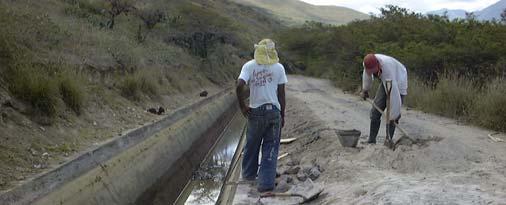
110 III. Photographs of BCW Construction Gary P. Merkley 102 BIE 5300/6300 Lectures

111 BIE 5300/6300 Lectures 103 Gary P. Merkley

112 Gary P. Merkley 104 BIE 5300/6300 Lectures

113 References & Bibliography BIE 5300/6300 Lectures 105 Gary P. Merkley

114 Gary P. Merkley 106 BIE 5300/6300 Lectures

115 Lecture 11 Calibration of Canal Gates I. Suitability of Gates for Flow Measurement Advantages relatively low head loss often already exists as a control device sediment passes through easily Disadvantages usually not as accurate as weirs floating debris tends to accumulate calibration can be complex for all flow conditions II. Orifice and Non-Orifice Flow Canal gates can operate under orifice flow conditions and as channel constrictions In general, either condition can occur under free or submerged (modular or non-modular) regimes Orifice flow occurs when the upstream depth is sufficient to seal the opening in other words, the bottom of the gate is lower than the upstream water surface elevation The difference between free and submerged flow for a gate operating as an orifice is that for free flow the downstream water surface elevation is less than CcG o, where C c is the contraction coefficient and G o is the vertical gate opening, referenced from the bottom of the gate opening (other criteria can be derived from momentum principles) The distinguishing difference between free and submerged flow in a channel constriction is the occurrence of critical velocity in the vicinity of the constriction (usually a very short distance upstream of the narrowest portion of the constriction) This lecture focuses on the calibration of gates under non-orifice flow conditions BIE 5300/6300 Lectures 107 Gary P. Merkley

116 III. Rating Open Channel Constrictions Whenever doing structure calibrations, examine the data carefully and try to identify erroneous values or mistakes Check the procedures used in the field or laboratory because sometimes the people who take the measurements are not paying attention and make errors Never blindly enter data into a spreadsheet or other computer program and accept the results at face value because you may get incorrect results and not even realize it Always graph the data and the calibration results; don t perform regression and other data analysis techniques without looking at a graphical representation of the data and comparison to the results Free Flow Gates perform hydraulically as open channel constrictions (non-orifice flow) when the gate is raised to the point that it does not touch the water surface The general form of the free-flow equation is: Q f n f f u = C h (1) where the subscript f denotes free flow; Q f is the free-flow discharge; C f is the free-flow coefficient; and n f is the free-flow exponent The value of C f increases as the size of the constriction increases, but the relationship is usually not linear The value of n f is primarily dependent upon the geometry of the constriction with the theoretical values being 3/2 for a rectangular constriction and 5/2 for a triangular constriction Sample Free-Flow Constriction Calibration Sample field data for developing the discharge rating for a rectangular openchannel constriction are listed in the table below The discharge rate in the constriction was determined by taking current meter readings at an upstream location, and again at a downstream location Gary P. Merkley 108 BIE 5300/6300 Lectures

117 This is a good practice because the upstream and downstream flow depths are often significantly different, so that the variation in the measured discharge between the two locations is indicative of the accuracy of the current meter equipment and the methodology used by the field staff Date Discharge Water Surface Elevation (m 3 /s) in Stilling Well (m) 21 Jun Jun Jun Jun Note: The listed discharge is the average discharge measured with a current meter at a location 23 m upstream of the constriction, and at another location 108 m downstream. The free-flow equation for the flow depths measured below the benchmark (at m) is: Q f = 0.74 h ( ) 1.55 u x (2) Col. 1 Col. 2 Col. 3 Col. 4 Col. 5 Discharge Water Surface (h u ) sw Tape Measurement (h u ) x (m 3 /s) Elevation (m) (m) (m) (m) Notes: The third column values equal the values in column 2 minus the floor elevation of m. The values in column 5 equal the benchmark elevation of m minus the floor elevation of m, minus the values in column 4. The Tape Measurement in the above table is for the vertical distance from the benchmark down to the water surface If a regression analysis is performed with the free-flow data using the theoretical value of n f = 3/2, or, Q Q = 0.73 h ( ) 1.5 f u sw (3) f ( ) 1.5 = 0.75 hu (4) x The error in the discharge resulting from using n f = 3/2 varies from -1.91% to +2.87%. BIE 5300/6300 Lectures 109 Gary P. Merkley

118 Submerged Flow The general form of the submerged-flow equation is: Q s( u d) ( logs) C h h = s n s n f (5) where the subscript s denotes submerged flow, so that Q s is the submerged-flow discharge, C s is the submerged-flow coefficient, and n s is the submerged-flow exponent Base 10 logarithms have usually been used with Eq. 5, but other bases could be used, so the base should be specified when providing calibration values Note that the free-flow exponent, n f, is used with the term h u - h d Consequently, n f is determined from the free-flow rating, while C s and n s must be evaluated using submerged-flow data The theoretical variation in n s is between 1.0 and 1.5 Note that the logarithm term in the denominator of Eq. 5 can be estimated by taking the first two or three terms of an infinite series (but this is not usually necessary): log e(1 + x) = x x + x x + (6) Graphical Solution for Submerged-Flow Calibration The graphical solution used to be performed by hand on log-log paper before PCs and programmable calculators became widely available This is essentially how the form of the submerged-flow equation was derived in the 1960 s This solution technique assumes that the free-flow exponent, n f, is known from a prior free-flow calibration at the same structure So, assuming you already know n f, and you have data for submerged flow conditions, you can plot Q s versus (h u h d ), as shown in the figure below where there are five measured points Gary P. Merkley 110 BIE 5300/6300 Lectures

119 The above graph has a log-log scale The slope of the parallel lines is equal to n f, as shown above (measured using a linear, not log, scale), and each line passes through one of the plotted data points The five values of Q s at each of the horizontal dashed lines are for h = 1.0 Get another sheet of log-log paper and plot the five Q h = 1.0 values versus - log 10 S, as shown in the figure below Draw a straight line through the five data points and extend this line to log 10 S = 1.0 (as shown above) The value on the ordinate at log 10 S = 1.0 is Cs The slope of the line is n s (measured with a linear scale) You might not prefer to use this method unless you have no computer BIE 5300/6300 Lectures 111 Gary P. Merkley

120 Submerged-Flow Calibration by Multiple Regression Multiple regression analysis can be used to arrive directly at all three values (C s, n f, and n s ) without free-flow data This can be done by taking the logarithm of Eq. 5 as follows: ( ) ( ) logq = logc + n log h h n log logs (7) s s f u d s Equation 7 is linear with respect to the unknowns C s, n f, and n s Such a procedure may be necessary when a constriction is to be calibrated in the field and only operates under submerged-flow conditions You can also compare the calculated n f values for the free- and submerged-flow calibrations (they should be nearly the same) Spreadsheet applications and other computer software can be used to perform multiple least-squares regression conveniently This method can give a good fit to field or laboratory data, but it tends to complicate the calculation of transition submergence, which is discussed below Sample Submerged-Flow Constriction Calibration In this example, a nearly constant discharge was diverted into the irrigation channel and a check structure with gates located 120 m downstream was used to incrementally increase the flow depths Each time that the gates were changed, it took 2-3 hours for the water surface elevations upstream to stabilize Thus, it took one day to collect the data for a single flow rate The data listed in the table below were collected in two consecutive days Date Discharge Tape Measurement Tape Measurement (m 3 /s) from U/S Benchmark (m) from D/S Benchmark (m) 22 Jun Jun Jun Jun Jun Jun Jun Jun Jun Jun Gary P. Merkley 112 BIE 5300/6300 Lectures

121 Q s (h u ) x (h d ) x (m 3 /s) (m) (m) S -log 10 S Q h= A logarithmic plot of the submerged-flow data can be made Each data point can have a line drawn at a slope of n f = 1.55 (from the prior freeat flow data analysis), which can be extended to where it intercepts the abscissa h u - h d = 1.0 Then, the corresponding value of discharge can be read on the ordinate, which is listed as Q h=1.0 in the above table The value of Q h=1.0 can also be determined analytically because a straight line on logarithmic paper is an exponential function having the simple form: then, or, s( u d) ns ( logs) nf s () ns ( logs) C h h nf Qs = = u Q h= 1 C 1 ( ) n s h= 1.0 u d f Q = Q h h ( h h ) nf d (8) (9) Q h= 1.0= s n ( h h ) f u Q d (10) where Q h=1.0 has a different value for each value of the submergence, S Using the term Q h=1.0 implies that h u - h d = 1.0 (by definition); thus, Eq. 10 reduces to: BIE 5300/6300 Lectures 113 Gary P. Merkley

122 s ( ) ( h h ) n f C 1.0 ns Q = = C logs (11) h= 1.0 u nf d s ( ) Again, this is a power function where Q h=1.0 can be plotted against (-log S) on logarithmic paper to yield a straight-line relationship Note that the straight line in such a plot would have a negative slope (-n s ) and that C s is the value of Q h=1.0 when (-log S) is equal to unity For the example data, the submerged-flow equation is: Q ( u d) ( logs) h h = s (12) Transition Submergence By setting the free-flow discharge equation equal to the submerged-flow discharge equation, the transition submergence, S t, can be determined Consider this: then, n ( ) ( logs ) f nf n C f s 1 St hu f u = ns t Ch ns ( ) ( ) ( ) t f t s t nf f S = C logs C 1 S = 0 (13) (14) In our example, we have: or, and, ( ) = ( ) logs S 0.74h ( u d) ( logs) h h u = 1.37 ( ) = ( ) logs S (15) (16) (17) The value of S in this relationship is S t provided the coefficients and exponents have been accurately determined Again, small errors will dramatically affect the determination of S t Gary P. Merkley 114 BIE 5300/6300 Lectures

123 ( ) ( ) t t 0.74 logs = S (18) Equation 18 can be solved to determine the value of S t, which in this case is 0.82 Thus, free flow exists when S < 0.82 and submerged flow exists when the submergence is greater than 82% The table below gives the submergence values for different values of Q s /Q f for the sample constriction rating S Q s /Q f S Q s /Q f f ( u d) ( logs) 1.55 Qs h h 1 = = Q 0.74h u (19) which is also equal to: Q Q s f = ( ) ( logs) S (20) For example, if h u and h d are measured and found to be and 1.337, the first step would be to compute the submergence, S, S = = (21) Thus, for this condition submerged flow exists in the example open-channel constriction In practice, there may only be a trivial solution for transition submergence, in which S t = 1.0. In these cases, the value of C s can be slightly lowered to obtain another mathematical root to the equation. This is a tweaking procedure. Note that it is almost always expected that 0.50 < S t < If you come up with a value outside of this range, you should be suspicious that the data and or the analysis might have errors. BIE 5300/6300 Lectures 115 Gary P. Merkley

124 IV. Constant-Head Orifices A constant-head orifice, or CHO, is a double orifice gate, usually installed at the entrance to a lateral or tertiary canal This is a design promoted for years by the USBR, and it can be found in irrigation canals in many countries The idea is that you set the downstream gate as a meter, and set the upstream gate as necessary to have a constant water level in the mid-gate pool It is kind of like the double doors in the engineering building at USU: they are designed to act as buffers people enter an exit the whereby the warm air doesn t escape so easily when building But, in practice, CHOs are seldom used as intended; instead, one of the gates is left wide open and the other is used for regulation (this is a waste of materials because one gate isn t used at all) Note the missing wheel in the upstream gate, in the above figure Few people know what CHOs are for, and even when they do, it is often considered inconvenient or impractical to operate both gates But these gates can be calibrated, just as with any other gate V. General Hydraulic Characteristics of Gates for Orifice Flow It is safe to assume that the exponent on the head for orifice flow (free and submerged) is 0.50, so it is not necessary to treat it as an empirically-determined calibration parameter The basic relationship for orifice flow can be derived from the Bernoulli equation For orifice flow, a theoretical contraction coefficient, C c, of is equal to π/(π+2), derived from hydrodynamics for vertical flow through an infinitely long slot Field-measured discharge coefficients for orifice flow through gates normally range from 0.65 to about 0.9 there is often a significant approach velocity Radial gates can be field calibrated using the same equation forms as vertical sluice gates, although special equations have been developed for them Gary P. Merkley 116 BIE 5300/6300 Lectures

125 VI. How do You Know if it is Free Flow? If the water level on the upstream side of the gate is above the bottom of the gate, then the flow regime is probably that of an orifice In this case, the momentum f unction (from open-channel hydraulics) can be used to determine whether the flow is free or submerged In some cases it will be obviously free flow or obviously submerged flow, but the following computational procedure is one way to distinguish between free orifice and submerged orifice flow In the figure below, h 1 is the depth just upstream of the gate, h 2 is the depth just downstream of the gate (depth at the vena-contracta section) and h 3 is the depth at a section in the downstream, a short distance away from the gate If the value of the momentum function corresponding to h 2 is greater than that corresponding to h 3, free flow will occur; otherwise, it is submerged The momentum function is: 2 Q M= Ahc + (22) ga where A is the cross-sectional area and h c is the depth to the centroid of the area from the water surface The following table shows the values of A and Ah c for three different channel sections BIE 5300/6300 Lectures 117 Gary P. Merkley

126 Section A Ah c Rectangular Trapezoidal bh m1+ m2 b+ h h 2 2 bh b m1+ m2 h h D ( ) ( )( ) Circular ( sin ) 3 8 θ θ D sin θ / 2 cos θ/ 2 θ sinθ For rectangular and trapezoidal sections, b is the base width For trapezoidal sections, m 1 and m 2 are the inverse side slopes (zero for vertical sides), which are equal for symmetrical sections For circular sections, θ is defined as: 1 2h θ= 2cos 1 D where D is the inside diameter of the circular section There are alternate forms of the equations for circular sections, but which yield the same calculation results. The depth h 2 can be determined in the either of the following two ways: 1. h 2 = C c G o where C c is the contraction coefficient and G o is the vertical gate opening 2. Equate the specific energies at sections 1 and 2, where 2 Q E = h+, then solve for h 2gA 2 2 Calculate M 2 and M 3 using the depths h 2 and h 3, respectively If M 2 M 3, the flow is submerged; otherwise the flow is free Another (simpler) criteria for the threshold between free- and submerged-orifice flow is: CG where C c is the contraction coefficient ( 0.61) c o = hd (23) Gary P. Merkley 118 BIE 5300/6300 Lectures

127 But this is not the preferred way to make the distinction and is not as accurate as the momentum-function approach VII. How do You Know if it is Orifice Flow? The threshold between orifice and nonorifice flow can be defined as: Ch o u = Go (24) where C o is an empirically-determined coefficient (0.80 C o 0.95) Note that if C o = 1.0, then when h u = G o, the water surface is on the verge of going below the bottom of the gate (or vice-versa), when the regime would clearly be nonorifice However, in moving from orifice to nonorifice flow, the transition would begin before this point, and that is why C o must be less than 1.0 It seems that more research is needed to better defined the value of C o In practice, the flow can move from any regime to any other at an underflow (gate) structure: Orifice Free FO Submerged SO Non-orifice FN SN VII. Orifice Ratings for Canal Gates For free-flow conditions through an orifice, the discharge equation is: Q f = CdCvA 2ghu (25) where C d is the dimensionless discharge coefficient; C v is the dimensionless velocity head coefficient; A is the area of the orifice opening, g is the ratio of weight to mass; and h u is measured from the centroid of the orifice to the upstream water level BIE 5300/6300 Lectures 119 Gary P. Merkley

128 The velocity head coefficient, C v, approaches unity as the approach velocity to the orifice decreases to zero In irrigation systems, C v can usually be assumed to be unity since most irrigation channels have very flat gradients and the flow velocities are low The upstream depth, h u, can also be measured from the bottom of the orifice opening if the downstream depth is taken to be about 0.61 times the vertical orifice opening Otherwise, it is assumed that the downstream depth is equal to one-half the opening, and h u is effectively measured from the area centroid of the opening The choice will affect the value of the discharge coefficient If h u is measured from the upstream canal bed, Eq. 4 becomes Qf = CdCvA 2g(hu CgGo) (26) where C g is usually either 0.5 or 0.61, as explained above. If the downstream water level is also above the top of the opening, submerged conditions exist and the discharge equation becomes: ( ) Q = C C A 2g h h (27) s d v u d where h u - h d is the difference in water surface elevations upstream and downstream of the submerged orifice. An orifice can be used as an accurate flow measuring device in an irrigation system If the orifice structure has not been previously rated in the laboratory, then it can easily be rated in the field As mentioned above, the hydraulic head term, (h u - C g G o ) or (h u - h d ), can be relied upon to have the exponent ½, which means that a single field rating measurement could provide an accurate determination of the coefficient of discharge, C d However, the use of a single rating measurement implies the assumption of a constant C d value, which is not the case in general Adjustments to the basic orifice equations for free- and submerged-flow are often made to more accurately represent the structure rating as a function of flow depths and gate openings The following sections present some alternative equation forms for taking into account the variability in the discharge coefficient under different operating conditions Gary P. Merkley 120 BIE 5300/6300 Lectures

129 VIII. Variation in the Discharge Coefficient Henry (1950) made numerous laboratory measurements to determine the discharge coefficient for free and submerged flow through an orifice gate The figure below shows an approximate representation of his data BIE 5300/6300 Lectures 121 Gary P. Merkley

130 Gary P. Merkley 122 BIE 5300/6300 Lectures

131 Lecture 12 Calibration of Canal Gates I. Free-Flow Rectangular Gate Structures For a rectangular gate having a gate opening, G o, and a gate width, W, the freelecture, flow discharge equation can be obtained from Eq. 26 of the previous assuming that the dimensionless velocity head coefficient is equal to unity: ( ) Q = C G G 2g h C G (1) f d o w u g o where G o is the vertical ga te open ing; G w is the gate width; GoG w is the area, A, of the gate opening; and, C g is betwe en 0.5 and The upstream flow depth, h u, can be measured anywhere upstream of the gate, including the u pstream face o f the gate The value of h u will vary only a small amount depending on the upstream location chosen for me asuring h u Consequen tly, the value of the coeffi cient of discharge, C d, will also vary according to the location selected for measuring hu One of the most difficult ta sks in calibratin g a gate st ructure is obtaining a highly accurate measurement of the gate openin g, G o For gates having a threaded rod th at rises as the gate ope ning is increased, the gate opening is read from the top of the hand-wheel to the top of the rod with the gate closed, and whe n set to some openin g, G o This very likely represents a measurement of gate opening from where the gate is totally seated, rather tha n a measureme nt from the gate lip; therefore, the measured value of G o from the threa d rod will usu ally be greater than the true gate opening, unless special precautions are taken to calibrate the thread rod Also, when the gate lip is set at the same elevation as the gate sill, there will undoubtedly be some flow or leakage through the gate This implies that the datum for measuring the gate opening is below the gate sill In fact, there is often leakage from a gate even when it is totally seated because of inadequate maintenance An example problem will be used to illustrate the procedure for determining an appropriate zero datum for the gate opening Sample Calibration Calibration data (listed in the table below) were collected for a rectangular gate structure The data reduction is listed in the next table, where the coefficient of discharge, C d, was calculated from Eq. 27 BIE 5300/6300 Lectures 123 Gary P. Merkley

132 Gate Opening, G o (m) Discharge, Q f (m 3 /s) Upstream Benchmark Tape Measurement (m) Q f (m 3 /s) G o (m) h u (m) Note: The discharge coefficient, C d, was calculated using the following equation: G Qf = CdGoGw 2g hu 2 A rectangular coordinate plot of C d versus the gate opening, G o, is shown in the figure below 0.76 o C d Coefficient of discharge, Cd Gate opening, Go (m) Gary P. Merkley 124 BIE 5300/6300 Lectures

133 Notice that the value of C d continues to decrease with larger gate openings One way to determine if a constant value of C d can be derived is to rewrite Eq. 5 in the following format (Skogerboe and Merkley 1996): Go + ( ) ( ) Qf = Cd Go + Go Gw 2g hu G o 2 G o (2) where G o is a measure of the zero datum level below the gate sill, and ( h ) u Go = h + (3) u G o Assuming values of G o equal to 1 mm, 2 mm, 3 mm, etc., the computations for determining C d can be made from Eq. 3 The results for G o equal to 1 mm, 2 mm, 3 mm, 4 mm, 5 mm, 6 mm, 7 mm, 8 mm and 12 mm (gate seated) are listed in the table below The best results are obtained for G o of 3 mm the results are plotted in the figure below, which shows that C d varies from to with the average value of C d being For this particular gate structure, the discharge normally varies between 200 and 300 lps, and the gate opening is normally operated between mm, so that a constant value of C d = can be used when the zero datum for G o and h u is taken as 3 mm below the gate sill Another alternative would be to use a constant value of C d = for G o = 4 mm and G o greater than 30 mm BIE 5300/6300 Lectures 125 Gary P. Merkley

134 Gary P. Merkley 126 BIE 5300/6300 Lectures

135 BIE 5300/6300 Lectures 127 Gary P. Merkley

136 II. Submerged-Flow Rectangular Gate Structures Assuming that the dimensionless velocity head coefficient in Eq. 27 is unity, the submerged-flow discharge equation for a rectangular gate having an opening, G o, and a width, W, becomes: ( ) Q = C G G 2g h h (4) s d o w u d where G o G w is the area, A, of the orifice Field calibration data for a rectangular gate structure operating under submerged-flow conditions are listed in the table below Note that for this type of slide gate, the gate opening can be measured both on the left side, (G o ) L, and the right side, (G o ) R, because the gate lip is not always horizontal The calculations are shown in the second table below Discharge, Q s (m 3 /s) (G o ) left (m) Gate Opening (G o ) right (m) Benchmark Tape Measurements Upstream (m) Downstream (m) Q s G o hu h d h u - h d (m 3 /s) (m) (m) (m) (m) C d As in the case of the free-flow orifice calibration in the previous section, a trialand-error approach can be used to determine a more precise zero datum for the gate opening In this case, the submerged flow equation would be rewritten as: ( ) ( Qs = Cd Go + Go Gw 2g hu d ) h (5) Gary P. Merkley 128 BIE 5300/6300 Lectures

137 where G o is the vertical distance from the gate sill down to the zero datum level, as previously defined in Eq. 2 Q s G o h u - h d C d (m 3 /s) (m) (m) G o = 4 mm G o = 6 mm G o = 8 mm Note: The discharge coefficient, C d, was calculated from Eq. 32: As before, the criteria for determining G o is to obtain a nearly constant value of the discharge coefficient, C d The above table has the example computational results for determining the discharge coefficient, C d, according to adjusted gate openings, G o, under submerged flow conditions III. Calibrating Medium- and Large-Size Gate Structures A different form of the submerged-flow rating equation has been used with excellent results on many different orifice-type structures in medium and large canals The differences in the equation involve consideration of the gate opening and the downstream depth as influential factors in the determination of the discharge coefficient The equation is as follows: ( ) Q = C h G 2g h h (6) s s s w u d and, C s β Go =α h (7) s where h s is the downstream depth referenced to the bottom of the gate opening, α and β are empirically-fitted parameters, and all other terms are as described previously BIE 5300/6300 Lectures 129 Gary P. Merkley

138 h u G o h s h d Note that C s is a dimensionless number The value of the exponent, β, is usually very close to unity In fact, for β equal to unity the equation reverts to that of a constant value of C s equal to α (the h s term cancels) The next table shows some example field calibration data for a large canal gate operating under submerged-flow conditions The solution to the example calibration is: α = 0.796, and β = This particular data set indicates an excellent fit to Eqs. 6 and 7, and it is typical of other large gate structures operating under submerged-flow conditions G o Data Discharge h Set (m 3 /s) (m) (m) (m) G o /h s C s Note: the data are for two identical gates in parallel, both having the same opening for each data set, with a combined opening width of 2.20 m. Gary P. Merkley 130 BIE 5300/6300 Lectures h s

139 A similar equation can be used for free-flow through a large gate structure, with the upstream depth, h u, replacing the term h s, and with (h u - G o /2) replacing (h u - h d ) As previously mentioned, the free-flow equation can be calibrated using (h u G o ) instead of (h u - G o /2) The following figure shows a graph of the 18 data points; the straight line is the regression results which gives α and β alpha = beta = s) ln(c ln(go/hs) IV. Radial Gate Orifice-Flow Calibrations This structure type includes radial (or Tainter ) gates as calibrated by the USBR (Buyalski 1983) for free and submerged orifice-flow conditions The calibration of the gates follows the specifications in the USBR REC-ERCsubmerged orifice flow, and corrections for the type of gate lip seal 83-9 technical publication, which gives calibration equations for free and The calibration requires no field measurements other than gate dimensions, but you can add another coefficient to the equations for free flow and orifice flow in an attempt to accommodate calibration data, if available Three gate lip seal designs (see figure below) are included in the calibrations: BIE 5300/6300 Lectures 131 Gary P. Merkley

140 1. Hard-rubber bar; 2. Music note; and, 3. Sharp edge The gate lip seal is the bottom of the gate leaf, which rests on the bottom of the channel when the gate is closed The discharge coefficients need no adjustment for the hard-rubber bar gate lip, which is the most common among USBR radial gate designs, but do have correction factors for the other two lip seal types These are given below for free and submerged orifice flow G r h u G o P h d The gate radius divided by the pinion height should be within the range 1.2 G r /P 1.7 The upstream water depth divided by the pinion height should be less than or equal to 1.6 (h u /P 1.6) If these and other limits are observed, the accuracy of the calculated flow rate from Buyalski s equations should be within 1% of the true flow rate Gary P. Merkley 132 BIE 5300/6300 Lectures

141 Free Orifice Flow Free, or modular orifice flow is assumed to prevail when the downstream momentum function corresponding to C c G o, where G o is the vertical gate opening, is less than or equal to the momentum function value using the downstream depth. Under these conditions the rating equation is: F f = Q f - CfcdaGoGw 2gh u = 0 (8) where C fcda is the free-flow discharge coefficient; G o is the vertical gate opening (m or ft); G w is the width of the gate opening (m or ft); and h u is the upstream water depth (m or ft); C fcda is dimensionless C fcda is determined according to a series of conic equations as defined by Buyalski (1983) from an analysis of over 2,000 data points The equations are lengthy, but are easily applied in a computer program Eccentricity 2 G AFE r = P + (9) 2 G BFE r = P (10) G o FE = AFE BFE P (11) Directrix where G r is the gate radius (m or ft); and P is the pinion height (m or ft) G AFD r = P 2 (12) BIE 5300/6300 Lectures 133 Gary P. Merkley

142 G r BFD = P (13) Go FD = BFD 1.0- AFD P 2 (14) Focal Distances Go Go FX1 = P P Go Go FX1 = > P P (15) and, Go FY1 = (16) P h FXV = u FX 1 P (17) The correction on C fcda for the music note gate lip seal design is: Go Ccorrect = (music note) P (18) The correction on C fcda for the sharp edge gate lip seal design is: Go Ccorrect = (sharp edge) P (19) For the hard-rubber bar gate lip seal design, C correct = 1.0. The preceding corrections on C fcda for the music note and sharp edge gate lip seal designs were chosen from the linear options proposed by Buyalski (ibid). Gary P. Merkley 134 BIE 5300/6300 Lectures

143 Finally, C = ( + ) fcda C correct FE FD FXV FXV + FY 1 (20) Radial gates in parallel at a check structure Submerged Orifice Flow The submerged orifice rating equation is: F s = Q s - Cscd a GG o w 2gh u = 0 (21) where C scda is the submerged-flow discharge coefficient; and all other terms are as previously defined; both Cscda and C ds are dimensionless Note that the square-root term does not include the downstream depth, hd, but it is included in the lengthy definition of C scda As in the free-flow case, C scda is determined according to a series of conic equations: Directrix G ADA = r 26.7 P 1 (22) BIE 5300/6300 Lectures 135 Gary P. Merkley

144 P ADB = (23) G r G AD = ADA o + ADB P 1 (24) G r BDA = P (25) G r BDB = (26) P G o BD = BDA P + BDB (27) h d DR = AD + BD P (28) D= DR (29) Eccentricity G r AEA = P (30) G r AEB = P (31) 1 G AE AEA o = + AEB P (32) Gary P. Merkley 136 BIE 5300/6300 Lectures

145 G r BEK = P (33) G BE = BEK o 0.44 P 2 (34) ER = AE( D) + BE (35) ER E = ln D (36) Vector V 1 Focal Distance 1 ( ) ED = E V (37) P AFA = (38) G r G r AFB = (39) P G o AF = AFA + AFB P (40) P BFA = Gr (41) BIE 5300/6300 Lectures 137 Gary P. Merkley

146 P BFB = (42) G r P BF = BFA + BFB Go (43) FY = BF ( ) AF h d P (44) If FY 0, then let FY = 0 and FX = 0. Otherwise, retain the calculated value of FY and, FX = V + FY V (for FY > 0) (45) hu hd VX = V1 FX P P (46) The correction on C scda for the music note gate lip seal design is: Go Ccorrect = (music note) P (47) The correction on C s cda for the shar p edge gate lip seal design is: Go Ccorrect = (sharp edge) P (48) For the hard-rubber bar gate lip seal design, C correct = 1.0 The preceding corrections on C scda for the music note and sharp edge gate lip seal designs were chosen from the linear options proposed by Buyalski (ibid) Finally, Gary P. Merkley 138 BIE 5300/6300 Lectures

147 2 2 2 Cscda = C correct E ( D + VX) VX + FY (49) References & Bibliography Buyalski, C.P Discharge algorithms for canal radial gates. Technical Report REC-ERC U.S. Bureau of Reclamation, Denver, CO. 232 pp. Brater, E.F., and H.W. King Handbook of hydraulics. 6 th edition. McGraw-Hill Book Company, New York, N.Y. 583 pp. Buyalski, C.P Discharge algorithms for canal radial gates. Technical Report REC-ERC U.S. Bureau of Reclamation, Denver, CO. 232 pp. Chow, V.T Open-channel hydraulics. McGraw-Hill Book Company, New York, N.Y. 680 pp. Daugherty, R.L., and J. B. Franzini Fluid mechanics with engineering applications. 7 th edition. McGraw-Hill Book Company, New York, N.Y. 564 pp. Davis, C.V. and K.E. Sorensen (eds.) Handbook of applied hydraulics. McGraw-Hill Book Company, New York, N.Y. French, R.H Open-channel hydraulics. McGraw-Hill Book Company, New York, N.Y. 705 pp. Hu, W.W Hydraulic elements for USBR standard horseshoe tunnel. J. of the Transportation Engrg. Div., ASCE, 99(4): Hu, W.W Water surface profile for horseshoe tunnel. Transportation Engrg. Journal, ASCE, 106(2): Press, W.H., S. A. Teukolsky, W. T. Vetterling, and B. P. Flannery Numerical recipes in C: the art of scientific computing. 2 nd Ed. Cambridge Univ. Press, Cambridge, U.K. 994 pp. Shen, J Discharge characteristics of triangular-notch thin-plate weirs. Water Supply Paper 1617-B. U.S. Geological Survey. Skogerboe, G.V., M.L. Hyatt, R.K. Anderson, and K.O. Eggleston Cutthroat flumes. Utah Water Research Laboratory Report WG pp. Skogerboe, G.V., L. Ren, and D. Yang Cutthroat flume discharge ratings, size selection and installation. Int l Irrig. Center Report, Utah State Univ., Logan, UT. 110 pp. Uni-Bell Plastic Pipe Association Handbook of PVC pipe: design and construction. Uni-Bell Plastic Pipe Association, Dallas, TX. Villamonte, J.R Submerged-weir discharge studies. Engrg. News Record, p BIE 5300/6300 Lectures 139 Gary P. Merkley

148 Gary P. Merkley 140 BIE 5300/6300 Lectures

149 Lecture 13 Flow Measurement in Pipes I. Introduction There are a wide variety of methods for measuring discharge and velocity in pipes, or closed conduits Many of these methods can provide very accurate measurements Others give only rough estimates But, in general, it is easier to obtain a given measurement accuracy in pipes when compared to measurement in open channels Some of the devices used are very expensive and are more suited to industrial and municipal systems than for agricultural irrigation systems II. Pitot Tubes The pitot tube is named after Henri Pitot who used a bent glass tube to measure velocities in a river in France in the 1700s The pitot tube can be used not only for measuring flow velocity in open channels (such as canals and rivers), but in closed conduits as well There are several variations of pitot tubes for measuring flow velocity, and many of these are commercially available Pitot tubes can be very simple devices with no moving parts More sophisticated versions can provide greater accuracy (e.g. differential head meters that separate the static pressure head from the velocity head) The pitot static tube, shown in the figure below, is one variation of the device which allows the static head (P/γ) and dynamic (total) head (P/γ + V 2 /2g) to be separately measured BIE 5300/6300 Lectures 141 Gary P. Merkley

150 The static head equals the depth if open-channel flow Calibrations are required because the velocity profile can change with the flow rate, and because measurement(s) are only a sampling of the velocities in the pipe The measurement from a pitot tube can be accurate to ±1% of the true velocity, even if the submerged end of the tube is up to ±15% out of alignment from the flow direction The velocity reading from a pitot tube must be multiplied by cross-sectional area to obtain the flow rate (it is a velocity-area method) Pitot tubes tend to become clogged unless the water in the pipe is very clean Also, pitot tubes may be impractical if there is a large head, unless a manometer is used with a dense liquid like mercury III. Differential Producers This is a class of flow measurement devices for full pipe flow Differential producers cause a pressure differential which can be measured and correlated to velocity and or flow rate in the pipe Examples of differential producers: Venturis Nozzles Orifices Measured P at a differential producer depends on: IV. Venturi Meters Flow rate Fluid properties Element geometry The principle of this flow measurement device was first documented by J.B. Venturi in 1797 in Italy Venturi meters have only a small head loss, no moving parts, and do not clog easily Gary P. Merkley 142 BIE 5300/6300 Lectures

151 The principle under which these devices operate is that some pressure head is converted to velocity head when the cross- sectional area of flow decreases (Bernoulli equation) Thus, the head differential can be measured between the upstream section and the throat section to give an estimation of flow velocity, and this can be multiplied by flow area to arrive at a discharge value The converging section is usually about 21º, and the diverging section is usually from 5 to 7º h Head loss 21º 5 º - 7º D 1 D 2 Flow D 1 A form of the calibration equation is: Q= CA 2 2g h(sg 1) 1 β 4 (1) where C is a dimensionless coefficient from approximately (small throat velocity and diameter) to (large throat velocity and diameter); β is the ratio of D 2 /D 1 ; D 1 and D 2 are the inside diameters at the upstream and throat sections, respectively; A 2 is the area of the throat section; h is the head differential; and sg is the specific gravity of the manometer liquid The discharge coefficient, C, is a constant value for given venturi dimensions Note that if D 2 = D 1, then β = 1, and Q is undefined; if D 0 > D 1, you get the square root of a negative number (but neither condition applies to a venturi) The coefficient, C, must be adjuste d to accommodate variations in water temperature BIE 5300/6300 Lectures 143 Gary P. Merkley

152 The value of β is usually between 0.25 and 0.50, but may be as high as 0.75 Venturi meters have been made out of steel, iron, concrete, wood, plastic, brass, bronze, and other materials Most modern venturi meters of small size are made from plastic (doesn t corrode) Many commercial venturi meters have patented features The upstream converging section usually has an angle of about 21 from the pipe axis, and the diverging section usually has an angle of 5 to 7 (1:6 divergence, as for the DS ramp of a BCW, is about 9.5 ) Straightening vanes may be required upstream of the venturi to prevent swirling flow, which can significantly affect the calibration It is generally recommended that there should be a distance of at least 10D 1 of straight pipe upstream of the venturi The head loss across a venturi meter is usually between 10 and 20% of h This percentage decreases for larger venturis and as the flow rate increases Venturi discharge measurement error is often within ±0.5% to ±1% of the true flow rate value V. Flow Nozzles Flow nozzles operate on the same principle as venturi meters, but the head loss tends to be much greater due to the absence of a downstream diverging section There is an upstream converging section, like a venturi, but there is no downstream diverging section to reduce energy loss Gary P. Merkley 144 BIE 5300/6300 Lectures

153 Flow nozzles can be less expensive than venturi meters, and can provide comparable accuracy The same equation as for venturi meters is used for flow nozzles The head differential across the nozzle can be measured using a manometer or some kind of differential pressure gauge The upstream tap should be within ½D 1 to D 1 upstream of the entrance to the nozzle The downstream tap should be approximately at the outlet of the nozzle (see the figure below) H GL Head loss Flow D 1 D 2 A Flow Nozzle in a Pipe The space between the nozzle and the pipe walls can be filled in to reduce the head loss through the nozzle, as seen in the following figure HGL Head loss Flow D 1 D 2 A Solid Flow Nozzle in a Pipe BIE 5300/6300 Lectures 145 Gary P. Merkley

154 VI. Orifice Meters These devices use a thin plate with an orifice, smaller than the pipe ID, to create a pressure differential The orifice opening is usually circular, but can be other shapes: Square Oval Triangular Others The pressure differential can be measured, as in venturi and nozzle meters, and the same equation as for venturi meters can be used However, the discharge coefficient is different for orifice meters It is easy to make and install an orifice meter in a pipeline easier than a nozzle Orifice meters can give accurate measurements of Q, and they are simple and inexpensive to build But, orifice meters cause a higher head loss than either the venturi or flow nozzle meters As with venturi meters and flow nozzles, orifice meters can provide values within ±1% (or better) of the true discharge As with venturi meters, there should be a straight section of pipe no less than 10 diameters upstream Some engineers have used eccentric orifices to allow passage of sediments the orifice is located at the bottom of a horizontal pipe, not in the center of the pipe cross section The orifice opening can be sharp (beveled) for better accuracy But don t use a beveled orifice opening if you are going to use it to measure flow in both directions These are the beveling dimensions: upstream downstream ½D D 1 to 0.02D 1 C L 30 to 45 deg ½D 2 Gary P. Merkley 146 BIE 5300/6300 Lectures

155 The upstream head is usually measured one pipe diameter upstream of the thin plate, and the downstream head is measured at a variable distance from the plate Standard calibrations are available, providing C values from which the discharge can be calculated for a given h value In the following, the coefficient for an orifice plate is called K, not C The coefficient values depend on the ratio of the diameters and on the Reynold s number of approach; they can be presented in tabular or graphical formats h Head loss vena contracta Flow D 1 D 2 D 1 0.5D 1 An Orifice Meter in a Pipe In the figure below, the Reynold s number of approach is calculated for the pipe section upstream of the orifice plate (diameter D 1, and the mean velocity in D 1 ) Note also that pipe flow is seldom laminar, so the curved parts of the figure are not of great interest An equation for use with the curves for K: Pu P Q KA d = 2 2g + zu + z d γ γ (2) The above equation is the same form as for canal gates operating as orifices The ratio β is embedded in the K term Note that z u equals z d for a horizontal pipe (they are measured relative to an arbitrary elevation datum) Note that P u /γ is the same as h u (same for P d /γ and h d ) Also, you can let h = h u - h d BIE 5300/6300 Lectures 147 Gary P. Merkley

156 P d is often measured at a distance of about ½D 1 downstream of the orifice plate, but the measurement is not too sensitive to the location, within a certain range (say ¼ D 1 to D 1 downstream) The following graph shows the K value for an orifice meter as a function of the ratio of diameters when the Reynold s number of approach is high enough that the K value no longer depends on R e 0.70 Orifice Meter Coefficient for High Reynold's Number K D 2 /D 1 Gary P. Merkley 148 BIE 5300/6300 Lectures

157 Orifice Plate Calibrations A perhaps better way to calibrate sharp-edged orifice plates in pipes is based on the following equations Flow rate can be calculated through the orifice using the following equation: Q= C A d 2 2g h(sg 1) 1 β 4 (3) where C d is a dimensionless orifice discharge coefficient, as defined below; A 2 is the cross-sectional area of the orifice plate opening; g is the ratio of weight to mass; h is the change in piezometric head across the orifice; and, β is a dimensionless ratio of the orifice and pipe diameters: β= D D 2 1 (4) where D 2 is the diameter of the circular orifice opening; and, D 1 is the inside di ameter of t he upstream pipe In Eq. 3, sg is the specific gravity of the manometer fluid, and the constant 1 represents the specific gravity of pure water The specific gravity of the manometer liquid must be greater than 1.0 Thus, if a manometer is used to measure the head differential across the orifice plate, th e term h(sg - 1) represents the head in depth (e.g. m or ft) of water If both ends of the manometer were open to the atmosphere, and there s no water in the manometer, then you will see h = 0 But if both ends of the manometer are open to the atmosphere, and you pour some water in one end, you ll see h > 0, thus the need for the (sg 1) term Note that the specific gravity of water can be slightly different than when the water is not pure, or when the water temperatu re is not exactly 5 C See the figure below Note al so that the manom eter liquid must not be water soluble! BIE 5300/6300 Lectures 149 Gary P. Merkley

158 flow Head of water = h(sg - 1) sg = 1 h sg > 1 The inside pipe diameter, D 1, is defined as: ( ) ( ) D1 = 1+αp T C 20 D1 (5) meas in which T C is the water temperature in C; (D 1 ) meas is the measured inside pipe diameter; and α p is the coefficient of linear thermal expansion of the pipe material (1/ C) The coefficient of linear thermal expansion is the ratio of the change in length per degree Celsius to the length at 0 C See the following table for linear thermal expansion values Gary P. Merkley 150 BIE 5300/6300 Lectures

159 Metal Plastic Other Material Coefficient of Linear Thermal Expansion (1/ C) Cast iron Steel Tin Copper Brass Aluminum Zinc PVC ABS PE Glass Wood Concrete For the range 0 to 100 C, the following two equations can be applied for the density and kinematic viscosity of water The density of pure water: ρ= (10) T (10) T (10) T + 1,000.2 (6) where ρ is in kg/m 3 ; and T is in C The kinematic viscosity of pure water: ν= T ,707.5T + 551,173 (7) where ν is in m 2 /s; and T is in C Similarly, the orifice diameter is corrected for thermal expansion as follows: ( ) ( ) D2 = 1+αop T C 20 D2 (8) meas where α op is the coefficient of linear thermal expansion of the orifice plate material (1/ C); and (D 2 ) meas is the measured orifice diameter Note that the water temperature must be substantially different than 20 C for the thermal expansion corrections to be significant The coefficient of discharge is defined by Miller (1996) for a circular pipe and orifice plate in which the upstream tap is located at a distance D 1 from the plate, and the downstream tap is at a distance ½D 1 : BIE 5300/6300 Lectures 151 Gary P. Merkley

160 C = β 0.184β d β 91.71β + β + 1 β R e (9) in which R e is the Reynolds number. Similar C d equations exist for other orifice plate configurations, and for venturis The C d expression for venturis is much simpler than that for orifice plates The Reynold s number is a function of the flow rate, so the solution is iterative The calculated value of C d is typically very near to 0.6, so if this is taken as the initial value, usually only one or two iterations are needed: References & Bibliography Miller, R.W Flow measurement engineering handbook. 3 rd Ed. McGraw-Hill Book Co., New York, N.Y. USBR Flow measurement manual. Water Resources Publications, LLC. Highlands Ranch, CO. 1. Specify T, h, α p, and α op 2. Calculate or specify ρ and ν 3. Calculate D 1 and D 2 4. Calculate β = D 1 /D 2 5. Let C d = Calculate Q 7. Calculate R e 8. Calculate C d Repeat steps 6-8 until Q converges to the desired precision Gary P. Merkley 152 BIE 5300/6300 Lectures

161 Lecture 14 Flow Measurement in Pipes I. Elbow Meters An elbow in a pipe can be used as a flow measuring device much in the same way as a venturi or orifice plate The head differential across the elbow (from inside to outside) is measured, and according to a calibration the discharge can be estimated The taps are usually located in the center of the elbow (e.g. at a 45 angle for a 90 elbow), but can be at other locations toward the upstream side of the elbow Some companies manufacture elbow meters for flow measurement, but almost any pipe elbow can be calibrated Elbow meters are not as potentially accurate as venturi, nozzle, and orifice meters Typical accuracy is about ±4% of Q One advantage of elbow meters is that there need not be any additional head loss in the piping system as a result of flow measurement The graph below is a sample calibration curve for a 1½-inch elbow meter in a USU hydraulic lab where the head differential (inside to outside tap) is measured in inches of mercury, using a manometer (data are from Dr. L.S. Willardson) 4.0 Calibration for a 1.5-inch Elbow Meter 3.5 Head differential (inches of Hg) Discharge (cfs) BIE 5300/6300 Lectures 153 Gary P. Merkley

162 II. Variable Area Meters These are vertical cylinders with a uniformly expanding cross-section in the upward direction A float inside the cylinder stabilizes at a certain elevation depending on the flow rate through the cylinder Note that the outside walls are usually transparent to allow direct readings by eye III. Horizontal Trajectory Method From physics, an accelerating object will travel a distance x in time t according to the following equation (based on Newton s 2 nd law): x 2 at = vot+ (1) 2 where x is the distance; v o is the initial velocity at time 0; t is the elapsed time; and a is the acceleration Flow emanating from a horizontal pipe will fall a height y over a distance x The horizontal component (x-direction) has almost no acceleration, and the vertical component (y-direction) has an initial velocity of zero The vertical acceleration is equal to the ratio of weight to mass, or g = 9.81 m/s 2 2 (32.2 ft/s ) Therefore, 2 gt x = vot and, y = (2) 2 Gary P. Merkley 154 BIE 5300/6300 Lectures

163 Then by getting rid of t, knowing that Q = VA, and the equation for the area of a circle, the flow rate is calculated as follows: Q = 2 πd x (3) 2y 4 g where D is the inside diameter of the circular pipe This equation is approximately correct if x and y are measured to the center of mass of the discharge trajectory Errors occur because in practice it is difficult to measure exactly to the center, and because of possible wind and other turbulent effects Also, the pipe might not be exactly horizontal (although a correction could take this into account, according to the same analysis given above) Tables of coefficient values derived from experiments allow x and y to be measured from the top of the trajectory However, measurements can be difficult because the flow is often very turbulent at a distance from the pipe end The previous equation can be simplified as: 2 x Q = 3.151CD (4) y where C is a coefficient to adjust the calculated discharge value when the ratios of x/d or y/d are smaller than 8 and 5, respectively (otherwise, C equals unity) Equation 4 is valid for x, y and D in ft, and Q in cfs The following table is for C values for use with Eq. 4 BIE 5300/6300 Lectures 155 Gary P. Merkley

164 y/d x/d This method can also be used for pipes flowing partially full (i.e. A < πd 2 /4), and experimental data are available to assist in the estimation of discharge for these conditions IV. California Pipe Method This is the horizontal pipe method for partially-full pipes It is somewhat analogous to the calibration for a weir or free overfall The following equation is in English units: 1 a Q = D (5) D where a and D are defined in the figure below (ft); and Q is discharge in cfs The ratio a/d is limited to: a/d > 0.45 This method was published in the 1920 s Measurement accuracy is only ±10%, at best The pipe must be exactly horizontal (level), with circular cross section The pipe must discharge freely into the air, unsubmerged Gary P. Merkley 156 BIE 5300/6300 Lectures

165 V. Vertical Trajectory Method As with pipes discharging horizontally into the air, there is a method to measure the flow rate from vertical pipes This is accomplished by assuming a translation of velocity head into the measurable height of a column of water above the top of the pipe Thus, to estimate the flow rate from pipes discharging vertically into the air it is only necessary to measure the: 1. inside diameter of the pipe, D; and, 2. the height of the jet, H, above the pipe This is a nice idea on paper, but in practice, it can be difficult to measure the height of the column of water because of sloshing, surging, and splashing Also, the act of measuring the height of the column can significantly alter the measured value The table below gives flow rate values in gpm for several pipe diameters in inches Jet Pipe Diameter (inch) Height (inch) (gpm) (gpm) (gpm) (gpm) (gpm) (gpm) (gpm) (gpm) ½ ½ ½ From Utah Engineering Experiment Station Bulletin 5, June Jet Height (first column) is the height from the top of the pipe to the top of the jet. BIE 5300/6300 Lectures 157 Gary P. Merkley

166 VI. Vortex Shedding Meters The vortex shedding meter can be accurate to within ±½% to ±1% of the true discharge The basic principal is that an object placed in the flow will cause turbulence and vortices in the downstream direction, and the rate of fluctuation of the vortices can be measured by detecting pressure variations just downstream This rate increases with increasing velocity, and it can be used to give an estimate of the discharge This requires calibration for a particular pipe material, pipe size, element shape and size, fluid type, and temperature It is essentially a velocity-area flow measurement method, but it is calibrated to give discharge directly Gary P. Merkley 158 BIE 5300/6300 Lectures

167 Vortex shedding meters are commercially available and are used with a variety of fluids, not only with water, and can operate well over a large pressure range and high flow velocities Size selection for these meters is important in order to avoid cavitation There need not be any moving parts in the meter This meter can be used for velocities up to approximately 50 m/s, or 180 kph The response of the device is linear for Reynolds numbers of 10,000 or more Errors can result from pipe vibration due to external machinery or other causes, or when the velocity is too low; however, some sophisticated devices have been developed and tested to correct for such errors VII. Ultrasonic Meters 1. Doppler An emitted pressure wave reflects off a deflector plate Difference between transmitted and reflected frequencies correlates to flow velocity Liquid does not have to be clean in fact, it may not work well if the liquid is too clean because it needs particles to reflect the signal 2. Transit-time Also called time-of-flight The liquid should be fairly clean with this method Devices generates high-frequency ( 1 MHz) pressure wave(s) Time to reach an opposing wall (inside the pipe) depends on: a) Flow velocity b) Beam orientation (angle) c) Speed of sound through the liquid medium Upstream straightening vanes may be needed to avoid swirling flow May have a single or multiple transmitted sound beams VIII. Other Measurement Devices Collins meters Commercial propeller flow meters Electromagnetic flow meters Volumetric tank BIE 5300/6300 Lectures 159 Gary P. Merkley

168 Weight tank References & Bibliography Brater, E.F. and H.W. King Handbook of hydraulics. McGraw-Hill. Daugherty, R.L. and J.B. Franzini Fluid mechanics with engineering applications. McGraw-Hill. Ginesi, D Putting new technology to work in flow measurement. Chilton s I&CS 60:2: Greve, F.W Measurement of pipe flow by the coordinate method. Purdue Engrg. Experiment Station Bulletin #32. Israelson, O.W. and V.E. Hansen Irrigation principles and practices. John Wiley, 3 rd Ed., pp King, L.G Drainage laboratory manual. BIE Dept., USU (BIE 605 course notes). Ledoux, J.W Venturi tube characteristics. Trans. ASCE, vol. 91. Lucas, G.P. and J.T. Turner Influence of cylinder geometry on the quality of its vortex shedding signal. Proc. Int l Conference on Flow Measurement (FLOWMECO 1985), Univ. of Melbourne, Australia, pp Miller, R.W Flow measurement engineering handbook. 3 rd Ed. McGraw-Hill Book Co., New York, N.Y. Sovik, R.E Flow measurement - some new considerations. Mech. Engrg., May, 107(5): Tily, P Practical options for on-line flow measurement. Process Engrg., London, 67(5): U.S. Bureau of Reclamation Water measurement manual. 2 nd Ed., Denver, CO. Gary P. Merkley 160 BIE 5300/6300 Lectures

169 Lecture 15 Canal Design Basics I. Canal Design Factors There are a number of criteria to consider when designing canals Below is a list of main criteria, not necessarily in order of importance: 1. Flow rate capacity requirements (demand) 2. Expected flow rate entering the canal (supply) 3. Construction cost 4. Safety considerations 5. Hydraulic operational characteristics 6. Water management needs 7. Maintenance requirements 8. Environmental conservation 9. Need for emergency spill structures 10. Cross-channel surface drainage needs 11. Need for drainage directed into the canal 12. Right-of-way (easements) along the canal path 13. Secondary uses (clothes washing, swimming, others) 14. Aesthetics Historically, flow rate capacity and construction cost have been the dominant design criteria, but it is better to take into account all of the above factors before finalizing a design This is not to say that you necessarily have to dwell on an issue like aesthetics, for example BIE 5300/6300 Lectures 161 Gary P. Merkley

170 However, issues such as dynamic operation, maintenance requirements and need for spillways have often been given only cursory attention during the design phase, requiring subsequent post-construction modifications to the infrastructure Water management and operational needs are very similar Secondary uses can include things like navigation (large canals), clothes washing, other domestic uses, aquatic production, bathing, and many others Remember that every design has both common and unique (site-specific) features, compared to other canals II. Capacity-Based Design This is an important consideration because a canal must have sufficient capacity, but not too much Construction and maintenance costs increase significantly with larger canals Actual required delivery system capacity depends on: 1. size of the irrigated area 2. cropping patterns (crop types, planting & rotation schedules) 3. climatological conditions 4. conveyance efficiencies 5. on-farm efficiencies 6. availability & exploitation of other water sources (conjunctive use) 7. type of delivery schedule (continuous, rotation, on-demand) 8. non-agricultural water needs It is often recommendable to allow for a safety factor by increasing capacities by 10% to 20% in case crops change, an expansion in irrigated area occurs, conveyance losses increase, and other possible factors The magnitude of design safety factors is very subjective and debatable Capacity requirements can change with different crop types, different total area, different planting schedules, and different efficiencies due to maintenance and rehabilitation (or lack thereof) On-demand delivery schedules require higher capacities because the combined requirements will tend to peak higher at some point during each growing season (on-demand delivery schemes can fail when there is not enough water or not enough conveyance capacity) Administrative losses can be significant, especially if the delivery schedule is very flexible (need extra water running through the system to buffer sudden turnout deliveries, else spill the excess) Gary P. Merkley 162 BIE 5300/6300 Lectures

171 The required design flow rate capacity is usually known from independent calculations For example, irrigation project canal capacities are based on peak crop evapotranspiration requirements and net irrigated area A typical main canal capacity is approximately 1 lps per irrigated hectare Irrigation canal capacity may also be partially based on non-irrigation requirements, such as municipal supply, industry, fishery & wildlife conservation, and others Of course, the capacity of the canals will depend on location, whereby the capacity requirements tend to decrease in the downstream direction due to deliveries in upstream reaches But, if the capacity for each reach is known based on crop water and other requirements, and one or more canal layouts have been identified, the design problem becomes one of cross-sectional shape and size, and longitudinal bed slope An important point in capacity-based designs is that most canal designs are static, based only on the hydraulic ability to carry up to a specified maximum flow rate The problem with this is that many designs did not consider the dynamics of canal operation, nor the type of delivery schedules envisioned This oversight has caused many operational difficulties and has limited the operational flexibility of many systems, sometimes severely The dynamics of canal operation can be taken into account through designphase modeling, either with physical models or mathematical models In earthen canals, and for canals in general, the most efficient cross section is a secondary consideration to erodibility, maintenance, safety, and convenience The ratio of flow depth, h, to canal bottom width, b, usually varies from 1:2 to 1:4 for small canals, and from 1:4 to 1:8 in large canals Freeboard can be designed into the canal size at ¼ of the maximum water depth plus one foot (maximum of 6 ft) Less freeboard is required if the canal is carefully controlled during operation Top width of the bank should allow for a vehicle to pass on one side; the other side can be more narrow III. System Layout Considerations A primary concern in the layout of the system is that it serves the purpose of conveying and distributing water to key locations in the area of service Another concern is that the excavation and earthen fill volumes not be excessive When large volumes of excavation and or fill are required, the construction costs can increase tremendously In fill areas, compaction of the soil material is very important, to avoid settlement problems and possible structural failure BIE 5300/6300 Lectures 163 Gary P. Merkley

172 In reaches constructed over fill, the seepage losses tend to be high, even if the canal is lined For these reasons, canals are often designed to follow the existing topography for the design bed slope, which often means routing the canals indirectly so that earth moving work can be minimized, or at least held to an acceptable level The selection of longitudinal bed slope should also take into account the existing slopes of the terrain, so as to minimize deviations in canal routing Curves in canals should not be too sharp; following are some recommended limits: Central Arizona Project canal (USBR) Channel Capacity (m 3 /s) Minimum Curve Radius (m) < ,000 > 90 1,500 In bends, the radius of curvature should usually be between 3 and 7 times the top width of flow at maximum design discharge (larger radius for larger canals) IV. Designing for Maximum Discharge and Uniform Flow For a known design discharge, known longitudinal bed slope, and selected crosssectional shape, the Manning or Chezy equation can be solved for the required depth Or, for a known design discharge, known longitudinal bed slope, and specified maximum depth, the Manning equation can be solved for the required base width of a rectangular section In general, the equation can be solved for any unknown, where all other parameters are specified You can also go to the field and measure everything but roughness under steady, uniform flow conditions, then calculate the value of n Avoid critical flow at or near design discharge (unstable water surface) V. Manning Equation The Manning equation has been used to size canals all over the world It is an empirical equation for approximating uniform flow conditions in open channels A roughness factor, n, is used in the equation Gary P. Merkley 164 BIE 5300/6300 Lectures

173 This factor is dependent on the type and condition of the canal lining But in reality, the factor also depends on the Reynold s number, N R (that is, the size and shape of the cross section, not just the roughness of the lining material) In practice, it is often erroneously assumed that n is independent of N R In Metric units: 1 Q AR S n 2/3 = o (1) where Q is in m 3 /s; A is cross-section flow area (m 2 ); R is hydraulic radius (m), equal to A divided by wetted perimeter; and S o is the longitudinal bed slope (dimensionless) In English units, a coefficient must be added to the equation: 1 ( m / ft) 1/ (2) In English units: /3 Q = AR S o (3) n where Q is in cfs; A is in ft 2 ; and R is in (ft) An alternative to the Manning equation is the Chezy equation VI. Chezy Equation The Chezy equation is an alternative to the Manning equation, and can be applied as described above It is also an empirical equation for approximating uniform flow conditions in open channels, but it has more of a theoretical basis The Chezy equation has a diagram analogous to the Moody diagram for the Darcy-Weisbach equation (pipe flow head loss) that takes the Reynold s number into account, which makes it technically more attractive than the Manning equation Another advantage is that the Chezy equation can be applied successfully on steeper slopes than the Manning equation Q = CA RS o (4) where Q is in m 3 /s; A is cross-section flow area (m 2 ); R is hydraulic radius (m), equal to A divided by wetted perimeter; and S o is the longitudinal bed slope (dimensionless) BIE 5300/6300 Lectures 165 Gary P. Merkley

174 VII. Chezy C Value The units of C are m ½ /s Note that the numerical value of C increases for smoother surfaces, which is opposite to the behavior of Manning s n The relationship between C and Manning s n is (for m and m 3 /s): The relationship between C and the Darcy-Weisbach f is: C C 1/ 6 R = (5) n 8g f (6) Thus, C can be defined as a function of relative roughness (ε/r) and Reynold s number, and the resulting graph looks much like the Moody diagram, vertically inverted Reynold s number can be defined like this: 4RV N = (7) ν R where R is the hydraulic radius (m), A/W p ; V is the mean flow velocity in a cross section (m/s); and ν is the kinematic viscosity of water (m 2 /s) For a full circle: 2 A πr r R = = = (8) W 2 π r 2 p whereby 4R = D (diameter), so use 4R in general for non-circular sections Kinematic viscosity is a function of water temperature Water Temperature ( C) Kinematic Viscosity (m 2 /s) Gary P. Merkley 166 BIE 5300/6300 Lectures

175 BIE 5300/6300 Lectures 167 Gary P. Merkley

176 For laminar flow (N R < 2000) and units of m and m 3 /s: C = N R (9) which is analogous to the Blasius equation (Darcy-Weisbach f) For turbulent smooth flow (N R > 2000 & ε 0) and units of m and m 3 /s: C 17.7 log 0.28C = 10 NR (10) For turbulent transitional flow (N R > 2000 & ε > 0) and units of m and m 3 /s: ε /R 0.28C C = 17.7 log NR (11) For turbulent rough flow (N R > 20,000 & ε > 0), where C is no longer a function of N R, and units of m and m 3 /s: C 17.7 log 12 ε /R = 10 (12) which gives the flat (horizontal) lines for fully turbulent flow To determine the threshold between turbulent transition and turbulent rough flow for a given ε/r ratio, first determine C from Eq. 11, then calculate N R as: N R 75C = (13) ε /R Other equations exist to define the C value as a function of N R and relative roughness, and these can be found in hydraulics textbooks & handbooks For R in ft, A in ft 2, and Q in cfs, multiply C by: That is, in English units: = (14) Q = 2.006CA RS o (15) Gary P. Merkley 168 BIE 5300/6300 Lectures

177 where Q is in cfs; A is in ft 2 ; and R is in ft Note that for all but laminar flow, you must iterate to solve for C This can be done quickly and easily in a computer program, and the results can be presented as in the graph above VIII. Chezy Epsilon Values Epsilon (roughness height) values depend on channel lining material type & condition: Material & Condition ε (m) Very smooth and essentially seamless concrete Smooth concrete with joints between panels Rough concrete surfaces Very rough concrete surfaces to Gunite with a smooth finish to Untreated gunite to References & Bibliography Davis, C.V. and K.E. Sorensen (eds.) Handbook of applied hydraulics. McGraw-Hill Book Company, New York, N.Y. Labye, Y., M.A, Olsen, A. Galand, and N. Tsiourtis Design and optimization of irrigation distribution networks. FAO Irrigation and Drainage Paper 44, Rome, Italy. 247 pp. USBR Design of small canal structures. U.S. Government Printing Office, Washington, D.C. 435 pp. BIE 5300/6300 Lectures 169 Gary P. Merkley

178 Gary P. Merkley 170 BIE 5300/6300 Lectures

179 Lecture 16 Channel Cross Sections I. Channel Cross Section Parameters Common cross-sectional shapes are rectangular, trapezoidal and circular Geometrically, rectangular cross-sections are just special cases of trapezoidal sections Circular cross sections are hydraulically more efficient than other crosssectional shapes, but they are only used for small channel sizes Circular cross sections are usually made of precast concrete mixes, and elevated above the ground Tunnels designed for open-channel flow are sometimes built with special cross sections (e.g. horseshoe sections) The standard horseshoe cross section has a semicircular top portion, and an intersection of three larger circles for the lower portion it can be considered a modification of a circular section A semi-circular channel cross section is the best shape for an open-channel, including open-channel flow in tunnels, but the horseshoe shape has been used in dozens of tunnels to allow for greater floor width, thereby facilitating the passage of equipment through the tunnel Standard horseshoe cross section (bold curves): diameter of upper section is half of the diameter of the three larger circles BIE 5300/6300 Lectures 171 Gary P. Merkley

180 Trapezoidal cross sections can be symmetrical or non-symmetrical For trapezoidal cross sections, the inverse side slope (H:V) is usually between zero and 2.0 Common inverse side slopes are zero (rectangular section), 1.0 and 1.5 There are tradeoffs between low and high values of side slope: 1. canals with low inverse side slopes occupy less land area 2. high inverse side slopes are more stable and may require less maintenance 3. high inverse side slopes are safer, if animals or people could fall into the canal, because it is easier to climb out 4. rectangular cross sections can be simpler to build, when lined with concrete (especially for small cross sections) 5. it may be easier to build and install structures and transitions for rectangular sections 6. medium-range side slopes correspond to greater hydraulic efficiency Compound sections are not uncommon For example, a combination of a trapezoidal and rectangular section: Gary P. Merkley 172 BIE 5300/6300 Lectures

181 II. Freeboard Recommendations Freeboard means the extra depth of a canal section, above the water surface for 100% flow rate capacity, usually for uniform-flow conditions A freeboard value should be added to the maximum expected depth to allow for: 1. deviations between design and construction (these are ubiquitous, only varying in magnitude from place to place) 2. post-construction, non-uniform land settlement 3. operational flexibility (including operator mistakes) 4. accommodate transient flow conditions 5. provide a more conservative design (in terms of flow capacity) 6. increase in hydraulic roughness due to lining deterioration, weed growth, and for other reasons 7. wind loading 8. other reasons Thus, with freeboard, under maximum flow conditions (full supply level, FSL), canal overflow is not impending If the canal starts to overflow, enormous erosive damage can occur in just a few minutes According to Murphy s Law, these things usually happen about 3:00 am, when no one is around. Then, everyone finds out at about 6:30 am after it has been spilling for hours. Many reaches of canal in many countries are routinely operated with virtually no freeboard, and disasters often occur BIE 5300/6300 Lectures 173 Gary P. Merkley

182 A canal which is overtopping the banks and spilling water. A canal with impending spillage (zero freeboard). Gary P. Merkley 174 BIE 5300/6300 Lectures

183 Traditional wisdom says that the minimum design freeboard for small canals is 1 ft ( m), so this would be the minimum for most any canal, but for very small canals it would certainly be excessive For canals with flow rates up to 3,000 cfs (85 m 3 /s), the freeboard should be up to 4 ft (1.2 m), and for intermediate flow rates, the freeboard should be 1 ft plus 25% of the maximum expected water depth However, the design freeboard can extend above the lined portion of a concretelined canal, and it often does (the berm of a lined canal is almost always higher than the top of the lining) Also, considerable judgment is required to know what the required freeboard might actually be, including knowledge of the operational modes in the canal (these will help determine the need for freeboard) Special analysis should go into the determination of required freeboard for canals with capacities exceeding 3,000 cfs, but such analysis can also be included for any size canal The analysis should also include economic criteria, because on large and or long canals, a difference of a few centimeters in freeboard is likely to mean a difference of millions of dollars in construction costs Nevertheless, the USBR published data on freeboard guidelines for up to 20,000 cfs (560 m 3 /s) capacities, and these are found in the plots below To put things in perspective, note that very few irrigation canals exceed a capacity of 100 m 3 /s; most main canals have a capacity of less than 20 m 3 /s BIE 5300/6300 Lectures 175 Gary P. Merkley

184 III. Trapezoidal Cross Section Symmetrical section: A = hb ( + mh) (16) T = b+ 2mh (17) p 2 W = b+ 2h m + 1 (18) Gary P. Merkley 176 BIE 5300/6300 Lectures

185 2 w h m 1 = + (19) m = h c T b 2 2 4w (T b) 2 h 2hm = b + 2A 3 (20) (21) h 2 h 4hm = b + 2A 3 (22) where h is the depth from the bottom (or invert ) of the cross section up to the centroid of the cross-sectional area; and h c is the depth from the water surface down to the area centroid: IV. Nonsymmetrical Trapezoidal Cross Section hc = h h (23) [ ] A = hb+ 0.5(m + m )h 1 2 ( ) T = b+ h m + m Wp = b+ h m m w = h m + 1 or h m + 1 (24) (25) (26) (27) BIE 5300/6300 Lectures 177 Gary P. Merkley

186 2 h h h = b m m 2A ( ) c h 2h h = b m m 2A ( ) 1 2 (28) (29) V. Circular Cross Section D T β h c h h In the following, angle β is in radians 1 2h β= 2cos 1 D (30) or, 2 D A = ( β sinβ ) (31) h r π A = (h r) 2hr h + r sin + r 2 (32) Gary P. Merkley 178 BIE 5300/6300 Lectures

187 where r = D/2 β 2h T = D sin D 1 = 1 2 D 2 (33) W p = βd 2 (34) D β h= 1 cos 2 2 (35) D 2 h = ( 2 hd h ) 3/2 2 3A (36) hc = h h (37) 7.0 Circular Channel with D = Beta, T, A, Wp beta Top Width Area Wetted Perimeter Hydraulic Radius Depth to Centroid Hydraulic radius & depth to centroid Depth Nondimensional curves of circular cross-section geometry. BIE 5300/6300 Lectures 179 Gary P. Merkley

188 VI. Standard Horseshoe Cross Section r r/2 h 3 h 2 h 1 The following is for a standard horseshoe cross section Divide the depth into three segments Note that h 1 + h 2 + h 3 = r (see the above figure) Determine h 1 by solving for the intersection of two of the circles then, 1+ 7 h1 = r 1 4 h r = h (38) (39) and, h 3 = r 2 (40) In the following, all angles are in radians Gary P. Merkley 180 BIE 5300/6300 Lectures

189 Top width (at water surface): For 0 < h h 1 : h T = 2r 1 1 r 2 (41) For h 1 < h r/2: or, r r 2 r r T = r h r h T = 2 r h r 2 2 r 2 (42) (43) For r/2 < h < r: 2h T = r 1 1 r 2 (44) and T = 0 when h = 0 or h = r Cross-sectional area: For 0 h h 1 : For h 1 < h r/2: 2 1 h r A = (h r) h( 2r h) + r sin + r π 2 (45) 2 1 A = r α2 α1 [ cot( α1) cot( α2) ] Aa + Ab + 4 A (46) where A 1 is the cross-sectional area corresponding to h = h 1 ; cot(α 1 ) is the cotangent of α 1, equal to 1/tan(α 1 ); and, 1 BIE 5300/6300 Lectures 181 Gary P. Merkley

190 2 2 r h2 ϕ 1 = (47) h 2 ϕ = 2 r 2 α = tan r h 2 r h 2 ( ϕ ) α = tan ( ϕ ) (48) (49) (50) and, 2 1 r r = Aa r h ϕ 2 1 r A = r h b 2 ϕ (51) (52) Note that h 2 = r/2-h 1 Note that α 1 and A b are constants for a given value of r Note that α 2 = π/2 and A a = 0 when h = r/2 Another way to calculate this (h 1 < h r/2) area is by integration: r A = 2 xdy+ A = 2 + r y dy A y2 y2 2 2 y y (53) which yields the following expression: y y A = ry+ y r y + r sin + A r y1 1 (54) where y 2 and y 1 are the integration limits: Gary P. Merkley 182 BIE 5300/6300 Lectures

191 r = (55) y2 h 2 y rc = (56) where, and, 1+ 7 C1 = C 1 C 1 1 C C = sin (57) (58) Finally, applying the integration limits: A = r C + sin h r r h + A 2r h r r 2 r 2 1 (59) where A 1 is the area corresponding to h = h 1 (Eq. 45) Equation 59 is preferred over Eq. 46 because it is simpler and yields the same result for h 1 < h r/2 For r/2 < h r: r r 1 2h r A = h h( r h) sin r where A 2 is the area corresponding to h = r/2 (Eq. 59) Depth to area centroid: For 0 h h 1 : ( ) r π 1 h h(2r h) 2 h = sin 1 hr 2h A 2 + r 3A A 2 (60) 3r (61) BIE 5300/6300 Lectures 183 Gary P. Merkley

192 where A is as calculated by Eq. 45; and h is the depth measured from the area centroid to the bottom of the cross section For h 1 < h r/2, the moment of area with respect to x is: Mx = ( yx) dy y = r + 2 r y x 2 2 ( ) 2 2 M = r ydy+ 2 y r y dy ry 2 Mx = r y /2 2 2 y2 y1 dy (62) where y 1 and y 2 are integration limits, exactly as defined above for crosssectional area. Applying the integration limits: where, r r 2 2 r x = 3 M r C h r h C C3 = C1 3/2 3/2 (63) (64) where C 3 is a constant; and C 1 is as defined in Eq. 57 The value of M x will be negative because it is calculated based on coordinate origins at h = r/2, so the depth to centroid for a given depth, h, must be shifted upward by the amount r/2: h x r M = + x (65) 2 A x which will be a positive value, with A x being the cross-sectional area corresponding to the same integration limits, y 1 and y 2 : 2 1 2h r r 2 r Ax = r C2 + sin h r r h 2r (66) and C 2 is also as previously defined Gary P. Merkley 184 BIE 5300/6300 Lectures

193 The composite value of h must account for the calculations up to h = h 1, so for depths from h 1 to r/2, the following area-weighted relationship is used to obtain the exact depth to the area centroid: h = r Mx Ax + + Ah 1 2 A 1 x A + A x 1 (67) where A 1 and h 1 are the values corresponding to h = h 1 (Eqs. 45 and 61) For r/2 < h r, the moment of area with respect to x is: 3 r 2 3/2 Mx = [ h(r h) ] (68) 12 3 The cross-sectional area from r/2 up to some h value is: r r 1 2h r Ax = h h(r h) + sin 2 4 r 2 (69) which is Eq. 60 minus the A 2 term The composite value of h must account for the calculations up to h = r/2, so for depths from r/2 to r, the following area-weighted relationship is used to obtain the exact depth to the area centroid: h = r Mx Ax + + Ah 2 2 A 2 x A + A x 2 (70) where A 2 and h 2 are the values corresponding to h = r/2 (Eqs. 59 and 67) Wetted perimeter: For 0 h h 1 : h 1 Wp = 2rcos 1 r (71) For h 1 < h r/2: BIE 5300/6300 Lectures 185 Gary P. Merkley

194 r 2h C 2r Wp = 2r cos cos Wp 1 + (72) where C 1 is as defined in Eq. 57; and W p1 is the wetted perimeter corresponding to h = h 1 (Eq. 71) Note that the term cos -1 (-C 1 /2) is a constant, based on h 1 For r/2 < h r: 2h π r 2 1 Wp = r cos 1 + Wp 2 (73) where W p2 is the wetted perimeter corresponding to h = r/2 (Eq. 72) 1.0 Standard Horseshoe Cross Section T/r, A/r 2, and h bar /r Top width Area Centroid depth Wetted perimeter W p /r Depth, h/r Nondimensional geometric values in a standard horseshoe cross section. The increase in area with the standard horseshoe cross section (compared to a circular section with a diameter of r) is only about 5.6% for a full section Gary P. Merkley 186 BIE 5300/6300 Lectures

195 VII. Efficient Canal Sections Sometimes it is useful to apply an efficient cross section to maximize channel capacity for a given bed slope and roughness However, other considerations such as side slope stability, safety, and lining material may be more important Comparisons between the most efficient section and other sections show that relative changes in the section often do not affect the capacity significantly capacity is much more sensitive to changes in roughness and bed slope VIII. Most Efficient Trapezoidal Canal Section How to calculate the most efficient trapezoidal cross section? Minimize the wetted perimeter with respect to cross-sectional area of flow (or depth), or maximize the hydraulic radius (R = A/W p ) Express the wetted perimeter as a function of A, m, and h, where h is depth Keep area, A, as a constant, otherwise you will get W p = 0 for the most efficient section Differentiate W p with respect to depth, h, and set it equal to zero For a symmetrical trapezoidal cross section: A = h(b + mh) (1) p 2 W = b+ 2h m + 1 (2) 1. Write the wetted perimeter in terms of A, h, and m (get rid of b by combining Eqs. 1 and 2): A b = mh (3) h A 2 Wp = mh+ 2h m + 1 (4) h 2. Differentiate W p with respect to h (A and m constant) and equate to zero (to minimize W p for a given area): Wp A 2 = 2 m + 2 m + 1 = 0 h h (5) BIE 5300/6300 Lectures 187 Gary P. Merkley

196 3. Solve Eq. 5 for A 2 2 A = h 2 m + 1 m (6) 4. For R = A/W p, use Eq. 6 to obtain R = 5. Now, manipulate Eq h 2 m + 1 m 2 b+ 2h m + 1 (7) R = 2 2 bh + 2h m + 1 bh mh 2 b+ 2h m (8) R = 2 h b 2h m h b+ mh 2 b+ 2h m + 1 ( ) (9) hwp A R = = h R (10) W p 6. Therefore, h = 2R, or, h R = (11) 2 You could also directly manipulate Eq. 6 to get the same result: 2A = hw p 7. For the most efficient rectangular section, A bh h R = = = W b + 2h 2 p (12) which results in b = 2h (bed width twice the maximum flow depth). 8. For the most efficient trapezoidal section we will get W p = T + b, where T is the top width of flow (b+2mh), which for a symmetrical trapezoid means that the length of each side slope (for depth h) is T/2. It also means that b = T/2, and this corresponds to half of a regular six-sided polygon, or a hexagon. The interior angle of a hexagon is 120 degrees, so m = 1/tan(60 ) = Gary P. Merkley 188 BIE 5300/6300 Lectures

197 IX. Parabolic Canal Section Suppose you have a parabolic channel section Define half of a symmetrical parabolic section as: h 2 = Kx (13) The cross-sectional area of flow (for half of the section) is: 3/2 h h h 2h A = x dh = dh = 0 0 K 3 K (14) The wetted perimeter (again, half of the section) is: p x 0 ( ) ( ) 2 ( ) 2 (15) W = lim f x + x f x + x or, W p 2 df = dx 1/ dx (16) where f = Kx 2. This derivation can be described graphically as follows: BIE 5300/6300 Lectures 189 Gary P. Merkley

198 where the curve is broken up (discretized) into successive linear segments ( ) ( ) ( s f x+ x f x + x (17) ) For y = f(x) = Kx 2, Then, W p 2 df 2 2 = 4K x dx (18) h/k 2 2 4K x 1dx (19) 0 = + After integration (using integration tables), the wetted perimeter for half of the parabolic section is: h h 1 1 h h 1 Wp = K ln 2K K + K K K K 2 4K 4K (20) which of course is a function of both K (curvature) and depth (h) An analysis of the hydraulic radius for such a parabolic section shows that the hydraulic radius decreases monotonically as K increases from an infinitesimally small value, so there is no most efficient value of K Chow (1959) has some equations (exact and approximate) for various channel section shapes, including the parabola defined in this case References & Bibliography Davis, C.V. and K.E. Sorensen (eds.) Handbook of applied hydraulics. McGraw-Hill Book Company, New York, N.Y. Hu, W.W Hydraulic elements for USBR standard horseshoe tunnel. J. of the Transportation Engrg. Div., ASCE, 99(4): Hu, W.W Water surface profile for horseshoe tunnel. Transportation Engrg. Journal, ASCE, 106(2): Labye, Y., M.A, Olsen, A. Galand, and N. Tsiourtis Design and optimization of irrigation distribution networks. FAO Irrigation and Drainage Paper 44, Rome, Italy. 247 pp. USBR Linings for irrigation canals. U.S. Government Printing Office, Washington, D.C. 149 pp. Gary P. Merkley 190 BIE 5300/6300 Lectures

199 Lecture 17 Design of Earthen Canals I. General Much of this information applies in general to both earthen and lined canals Attempt to balance cuts and fills to avoid waste material and or the need for borrow pits along the canal It is expensive to move earth long distances, and or to move it in large volumes Many large canals zigzag across the terrain to accommodate natural slopes; this makes the canal longer than it may need to be, but earthwork is less Canals may also follow the contours along hilly or mountainous terrain Of course, canal routing must also consider the location of water delivery points In hilly and mountainous terrain, canals generally follow contour gradients equal to the design bed slope of the canal Adjustments can be made by applying geometrical equations, but usually a lot of hand calculations and trial-and-error are required As previously discussed, it is generally best to follow the natural contour of the land such that the longitudinal bed slope is acceptable Most large- and medium-size irrigation canals have longitudinal slopes from to m/m A typical design value is m/m, but in mountainous areas the slope may be as high as m/m: elevation change is more than enough With larger bed slopes the problems of sedimentation can be lessened In the technical literature, it is possible to find many papers and articles on canal design, including application of mathematical optimization techniques (e.g. FAO Irrig & Drain Paper #44), some of which are many years old The design of new canals is not as predominant as it once was II. Earthen Canal Design Criteria A borrow pit An earthen channel Design cross sections are usually trapezoidal Field measurements of many older canals will also show that this is the range of averaged side slopes, even though they don t appear to be trapezoidal in shape BIE 5300/6300 Lectures 191 Gary P. Merkley

200 When canals are built on hillsides, a berm on the uphill side should be constructed to help prevent sloughing and landslides, which could block the canal and cause considerable damage if the canal is breached III. Earth Canal Design: Velocity Limitations In designing earthen canals it is necessary to consider erodibility of the banks and bed -- this is an empirical exercise, and experience by the designer is valuable Below are four methods applied to the design of earthen channels The first three of these are entirely empirical All of these methods apply to open channels with erodible boundaries in alluvial soils carrying sediment in the water 1. Kennedy Formula 1. Kennedy Formula 2. Lacey Method 3. Maximum Velocity Method 4. Tractive-Force Method Originally developed by British on a canal system in Pakistan Previously in wide use, but not used very much today V C h C ( ) 2 o = 1 avg (1) where V o is the velocity (fps); and h avg is the mean water depth (ft) The resulting velocity is supposed to be just right, so that neither erosion nor sediment deposition will occur in the channel The coefficient (C 1 ) and exponent (C 2 ) can be adjusted for specific conditions, preferably based on field measurements C 1 is mostly a function of the characteristics of the earthen material in the channel C 2 is dependent on the silt load of the water Below are values for the coefficient and exponent of the Kennedy formula: Table 1. Calibration values for the Kennedy formula. C 1 Material 0.56 extremely fine soil 0.84 fine, light sandy soil 0.92 coarse, light sandy soil 1.01 sandy, loamy silt 1.09 coarse silt or hard silt debris Gary P. Merkley 192 BIE 5300/6300 Lectures

201 C 2 Sediment Load 0.64 water containing very fine silt 0.50 clear water 1.2 Kennedy Formula (clear water: C 2 = 0.50) Velocity, V o (m/s) C1 = 0.56 C1 = 0.84 C1 = 0.92 C1 = 1.01 C1 = Depth, d b (m) Figure 1. Velocity values versus water depth for the Kennedy formula with clear water. 2. Lacey Method Developed by G. Lacey in the early part of the 20 th century based on data from India, Pakistan, Egypt and elsewhere Supports the Lindley Regime Concept, in which Lindley wrote: when an artificial channel is used to convey silty water, both bed and banks scour or fill, changing depth, gradient and width, until a state of balance is attained at which the channel is said to be in regime There are four relationships in the Lacey method All four must be satisfied to achieve regime conditions BIE 5300/6300 Lectures 193 Gary P. Merkley

202 1. Velocity 2. Wetted Perimeter 3. Hydraulic Radius 4. Bed Slope where, S V Wp = 1.17 fr (2) = 2.67 Q (3) R = Q/f (4) 2/3 f = (5) 1/ Q f = 1.76 d m (6) and, d m is the mean diameter of the bed and side slope materials (mm); V is the mean velocity over the cross-section (fps); W p is the wetted perimeter (ft); R is the hydraulic radius (ft); S is the longitudinal bed slope (ft/ft); and Q is discharge (cfs) The above relationships can be algebraically manipulated to derive other dependent relationships that may be convenient for some applications For example, solve for S in terms of discharge Or, solve for d m as a function of R and V Here are two variations of the equations: and, 11/12 V = d m / S 1/ 6 1/12 V = Q d m (7) (8) A weakness in the above method is that it considers particle size, d m, but not cohesion & adhesion Lacey General Slope Formula: V = R S (9) N a where N a is a roughness factor, defined as: N = f 0.9nR a (10) where n is the Manning roughness factor Gary P. Merkley 194 BIE 5300/6300 Lectures

203 This is for uniform flow conditions Applies to both regime and non-regime conditions Appears similar to the Manning equation, but according to Lacey it is more representative of flow in alluvial channels 3. Maximum Velocity Method This method gives the maximum permissible mean velocity based on the type of bed material and silt load of the water It is basically a compilation of field data, experience, and judgment Does not consider the depth of flow, which is generally regarded as an important factor in determining velocity limits Table 2. Maximum permissible velocities recommended by Fortier and Scobey Material Clear water Velocity (fps) Water with colloidal silt Fine sand, colloidal Sandy loam, non-colloidal Silt loam, non-colloidal 2 3 Alluvial silt, non-colloidal Firm loam soil Volcanic ash Stiff clay, highly colloidal Alluvial silt, colloidal Shales and hard "pans" 6 6 Fine gravel Coarse gravel 4 6 Cobble and shingle Table 3. USBR data on permissible velocities for non-cohesive soils Particle diameter (mm) Mean velocity (fps) Material Silt Fine sand Medium sand Coarse sand Fine gravel Medium gravel Coarse gravel Fine pebbles Medium pebbles Coarse pebbles Large pebbles BIE 5300/6300 Lectures 195 Gary P. Merkley

204 IV. Introduction to the Tractive Force Method This method is to prevent scouring, not sediment deposition This is another design methodology for earthen channels, but it is not 100% empirical, unlike the previously discussed methods It is most applicable to the design of earthen channels with erodible boundaries (wetted perimeter) carrying clear water, and earthen channels in which the material forming the boundaries is much coarser than the transported sediment The tractive force is that which is exerted on soil particles on the wetted perimeter of an earthen channel by the water flowing in the channel The tractive force is actually a shear stress multiplied by an area upon which the stress acts A component of the force of gravity on the side slope material is added to the analysis, whereby gravity will tend to cause soil particles to roll or slide down toward the channel invert (bed, or bottom) The design methodology treats the bed of the channel separately from the side slopes The key criterion is whether the tractive + gravity forces are less than the critical tractive force of the materials along the wetted perimeter of the channel If this is true, the channel should not experience scouring (erosion) from the flow of water within Thus, the critical tractive force is the threshold value at which scouring would be expected to begin This earthen canal design approach is for the prevention of scouring, but not for the prevention of sediment deposition The design methodology is for trapezoidal or rectangular cross sections This methodology was developed by the USBR V. Forces on Bed Particles The friction force (resisting particle movement) is: Ws tanθ (11) where θ is the angle of repose of the bed material and W s is the weight of a soil particle Gary P. Merkley 196 BIE 5300/6300 Lectures

205 Use the angle of repose for wet (not dry) material θ will be larger for most wet materials Note that tan θ is the angle of repose represented as a slope 42 Angle of Repose for Non-Cohesive Earthen Material Angle of repose (degrees) Very angular Moderately angular Slightly angular Slightly rounded Moderately rounded Very rounded Soil particle size (mm) 100 Figure 2. Angle of repose (degrees from horizontal), θ, for non-cohesive earthen materials (adapted from USBR Hyd Lab Report Hyd-366). The shear force on a bed particle is: at bed (12) where a is the effective particle area and T bed (lbs/ft 2 or N/m 2 ) is the shear stress exerted on the particle by the flow of water in the channel When particle movement is impending on the channel bed, expressions 1 and 2 are equal, and: or, W tanθ = at (13) s bed T bed W tanθ a = s (14) BIE 5300/6300 Lectures 197 Gary P. Merkley

206 VI. Forces on Side-Slope Particles The component of gravity down the side slope is: Ws sinφ (15) where φ is the angle of the side slope, as defined in the figure below Figure 3. Force components on a soil particle along the side slope of an earthen channel. If the inverse side slope is m, then: φ= tan m 1 1 (16) The force on the side slope particles in the direction of water flow is: at side (17) where T side is the shear stress (lbs/ft 2 or N/m 2 ) exerted on the side slope particle by the flow of water in the channel Note: multiply lbs/ft 2 by 47.9 to convert to N/m 2 Combining Eqs. 15 & 17, the resultant force on the side slope particles is downward and toward the direction of water flow, with the following magnitude: s φ+ a Tside (18) W sin The resistance to particle movement on the side slopes is due to the orthogonal component of Eq. 15, W s cosφ, as shown in the above figure, multiplied by the coefficient of friction, tan θ Thus, when particle movement is impending on the side slopes: Gary P. Merkley 198 BIE 5300/6300 Lectures

207 Solving Eq. 19 for T side : s s W cosφtanθ = W sin φ+ a Tside (19) Ws Tside = cos φtan θ sin φ (20) a Applying trigonometric identities and simplifying: 2 Ws t side = φ θ 2 T cos tan 1 a an φ tan θ (21) or, 2 Ws s side = θ 2 T tan 1 a in φ sin θ (22) VII. Tractive Force Ratio As defined in Eq. 14, T bed is the critical shear on bed particles As defined in Eqs , T side is the critical shear on side slope particles The tractive force ratio, K, is defined as: K T = side (23) T bed where T side and T bed are the critical (threshold) values defined in Eqs. 4 & 9-11 Then: 2 2 sin φ tan K = 1 = cosφ 1 sin θ tan 2 2 φ θ (24) VIII. Design Procedure The design procedure is based on calculations of maximum depth of flow, h Separate values are calculated for the channel bed and the side slopes, respectively BIE 5300/6300 Lectures 199 Gary P. Merkley

208 It is necessary to choose values for inverse side slope, m, and bed width, b to calculate maximum allowable depth in this procedure Limits on side slope will be found according to the angle of repose and the maximum allowable channel width Limits on bed width can be set by specifying allowable ranges on the ratio of b/h, where b is the channel base width and h is the flow depth Thus, the procedure involves some trial and error Step 0 Specify the desired maximum discharge in the channel Identify the soil characteristics (particle size gradation, cohesion) Determine the angle of repose of the soil material, θ Determine the longitudinal bed slope, S o, of the channel Step 1 Determine the critical shear stress, T c (N/m 2 or lbs/ft 2 ), based on the type of material and particle size from Fig. 3 or 4 (note: N/m 2 per lbs/ft 2 ) Fig. 3 is for cohesive material; Fig. 4 is for non-cohesive material Limit φ according to θ (let φ θ) Step 2 Choose a value for b Choose a value for m Step 3 Calculate φ from Eq. 16 Calculate K from Eq. 24 Determine the max shear stress fraction (dimensionless), K bed, for the channel bed, based on the b/h ratio and Fig. 6 Determine the max shear stress fraction (dimensionless), K side, for the channel side slopes, based on the b/h ratio and Fig. 7 Gary P. Merkley 200 BIE 5300/6300 Lectures

209 100 Permissible T c for Cohesive Material Tc (N/m 2 ) 10 Lean clay Clay Heavy clay Sandy clay Void Ratio Figure 4. Permissible value of critical shear stress, T c, in N/m 2, for cohesive earthen material (adapted from USBR Hyd Lab Report Hyd-352). About Figure 4: The void ratio is the ratio of volume of pores to volume of solids. Note that it is greater than 1.0 when there is more void space than that occupied by solids. The void ratio for soils is usually between 0.3 and 2.0. BIE 5300/6300 Lectures 201 Gary P. Merkley

210 100 Permissible T c for Non-Cohesive Material Clear water Low content of fine sediment High content of fine sediment Coarse, non-cohesive material Tc (N/m 2 ) 10 size for which gradation gives 25% of the material being larger in size Average particle diameter (mm) Figure 5. Permissible value of critical shear stress, T c, in N/m 2, for noncohesive earthen material (adapted from USBR Hyd Lab Report Hyd-352). The three curves at the left side of Fig. 5 are for the average particle diameter The straight line at the upper right of Fig. 5 is not for the average particle diameter, but for the particle size at which 25% of the material is larger in size This implies that a gradation (sieve) analysis has been performed on the earthen material particle gradation 75% 25% smallest largest Gary P. Merkley 202 BIE 5300/6300 Lectures

211 The three curves at the left side of Fig. 5 (d 5 mm) can be approximated as follows: Clear water: c 3 2 T = d d d (25) Low sediment: c 3 2 T = d 0.241d d (26) High sediment: 3 2 T = d d d c (27) where T c is in N/m 2 ; and d is in mm The portion of Fig 5. corresponding to coarse material (d > 5 mm) is approximated as: Coarse material: T = 2.17d c 0.75 (28) Equations are for diameter, d, in mm; and T c in N/m 2 Equations give T c values within ±1% of the USBR-published data Note that Eq. 28 is exponential, which is required for a straight-line plot with loglog scales BIE 5300/6300 Lectures 203 Gary P. Merkley

212 Figure 6. K bed values as a function of the b/h ratio. Notes: This figure was made using data from USBR Hydraulic Lab Report Hyd-366. The ordinate values are for maximum shear stress divided by γhs o, where γ = ρg, h is water depth, and S o is longitudinal bed slope. Both the ordinate & abscissa values are dimensionless. Gary P. Merkley 204 BIE 5300/6300 Lectures

213 Figure 7. K side values as a function of the b/h ratio. Notes: This figure was made using data from USBR Hydraulic Lab Report Hyd-366. The ordinate values are for maximum shear stress divided by γhs o, where γ = ρg, h is water depth, and S o is longitudinal bed slope. Both the ordinate and abscissa values are dimensionless. BIE 5300/6300 Lectures 205 Gary P. Merkley

214 Regression analysis can be performed on the plotted data for K bed & K side This is useful to allow interpolations that can be programmed, instead of reading values off the curves by eye The following regression results give sufficient accuracy for the max shear stress fractions: b Kbed for 1 b /h 4 h b Kbed for 4 b / h 10 h (29) for trapezoidal cross sections; and, K side AB+ B+ C( b/h) D ( b/h) D (30) where, 2 ( ) ( ) A = m m (31) ( ) B = e m 7.23 ( ) C = e m 5.63 D = e 35.2 m ( ) 3.29 (32) (33) (34) for 1 m 3, and where e is the base of natural logarithms Equations 29 give K bed to within ±1% of the values from the USBR data for 1 b/h 10 Equations give K side to within ±2% of the values from the USBR data for 1 m 3 (where the graphed values for m = 3 are extrapolated from the lower m values) The figure below is adapted from the USBR, defining the inverse side slope, and bed width The figure below also indicates locations of measured maximum tractive force on the side slopes, K side, and the bed, K bed These latter two are proportional to the ordinate values of the above two graphs (Figs. 6 & 7) Gary P. Merkley 206 BIE 5300/6300 Lectures

215 Step 4 Calculate the maximum depth based on K bed : h max = KTc K γs bed o (35) Recall that K is a function of φ and θ (Eq. 13) Calculate the maximum depth based on K side : h max = KTc K γs side o (36) where γ is 62.4 lbs/ft 3, or 9,810 N/m 3 Note that K, K bed, K side, and S o are all dimensionless; and T c /γ gives units of length (ft or m), which is what is expected for h The smaller of the two h max values from the above equations is applied to the design (i.e. the worst case scenario) Step 5 Take the smaller of the two depth, h, values from Eqs. 35 & 36 Use the Manning or Chezy equations to calculate the flow rate If the flow rate is sufficiently close to the desired maximum discharge value, the design process is finished If the flow rate is not the desired value, change the side slope, m, and or bed width, b, checking the m and b/h limits you may have set initially Return to Step 3 and repeat calculations There are other ways to attack the problem, but it s almost always iterative BIE 5300/6300 Lectures 207 Gary P. Merkley

216 For a very wide earthen channel, the channel sides become negligible and the critical tractive force on the channel bed can be taken as: T c γ hs (37) o Then, if S o is known, h can be calculated IX. Definition of Symbols a effective particle area (m 2 or ft 2 ) b channel base width (m or ft) h depth of water (m or ft) h max maximum depth of water (m or ft) K tractive force ratio (function of φ and θ) K bed maximum shear stress fraction (bed) K side maximum shear stress fraction (side slopes) m inverse side slope S o longitudinal bed slope T bed shear stress exerted on a bed soil particle (N/m 2 or lbs/ft 2 ) T c critical shear stress (N/m 2 or lbs/ft 2 ) T side shear stress exerted on a side slope soil particle (N/m 2 or lbs/ft 2 ) W s weight of a soil particle (N or lbs) φ inverse side slope angle γ weight of water per unit volume (N/m 3 or lbs/ft 3 ) θ angle of repose (wet soil material) References & Bibliography Carter, A.C Critical tractive forces on channel side slopes. Hydraulic Laboratory Report No. HYD-366. U.S. Bureau of Reclamation, Denver, CO. Chow, V.T Open-channel hydraulics. McGraw-Hill Book Co., Inc., New York, NY. Davis, C.S Handbook of applied hydraulics (2 nd ed.). McGraw-Hill Book Co., Inc., New York, NY. Labye, Y., M.A. Olson, A. Galand, and N. Tsiourtis Design and optimization of irrigation distribution networks. FAO Irrigation and Drainage Paper 44, United Nations, Rome, Italy. 247 pp. Lane, E.W Critical tractive forces on channel side slopes. Hydraulic Laboratory Report No. HYD-295. U.S. Bureau of Reclamation, Denver, CO. Lane, E.W Progress report on results of studies on design of stable channels. Hydraulic Laboratory Report No. HYD-352. U.S. Bureau of Reclamation, Denver, CO. Smerdon, E.T. and R.P. Beasley Critical tractive forces in cohesive soils. J. of Agric. Engrg., American Soc. of Agric. Engineers, pp Gary P. Merkley 208 BIE 5300/6300 Lectures

217 Lecture 18 Sample Earthen Channel Designs I. Example A : Design Procedure for an Earthen Canal Design an earthen canal section in an alluvial soil such that the wetted boundaries do not become eroded The canal will follow the natural terrain at an estimated S o = ft/ft with a preliminary design side slope of 1.5:1.0 (h:v) The bed material has been determined to be a non-cohesive coarse light sand with an average particle diameter of 10 mm, 25% of which is larger than 15 mm Thus, 15 mm will be used to determine T c in Fig. 5 Tests have shown that the angle of repose for the bed material is approximately 34, measured from the horizontal For the Manning equation, use a roughness value of The design discharge (Q max ) is 650 cfs The source of water is such that there will be a low content of fine sediment The canal can be assumed to be straight, even though there will be bends at several locations Design the section using a trapezoidal shape with a bed width to depth ratio, b/h, of between 1.0 and 5.0 The design should also be such that the canal bed and sides do not erode Adjust the side slope if necessary, but keep it within the range 0.5:1 to 2.0:1 (h:v) Note that φ < θ must be true to allow for a stable side slope 1. Design the canal using the tractive force method 2. Compare the results for the case in which it is assumed that the channel is very wide (i.e. critical tractive force = γhs o ) 3. Compare with results from the Kennedy formula 4. Compare with results from the Lacey method 5. Compare with results from the maximum velocity method using Table 2, and again using Table 3 Solution to Example A Design Problem: 1. Tractive Force Method Critical Tractive Force The critical tractive force can be estimated from Figure 5 (see above) The material is non-cohesive, and 25% of the particles are larger than 15 mm This gives T c 16.3 N/m 2 (0.34 lbs/ft 2 ) for the 15 mm abscissa value BIE 5300/6300 Lectures 209 Gary P. Merkley

218 Angle of Repose The angle of repose, θ, is given as 34 Then, the ratio of T side to T bed is: Tside sin φ K = = 1 = 1 3.2sin T 2 sin θ bed 2 2 φ (1) Design requirements for this example call for a side slope between 0.5 & 2.0 Actually, the range is restricted to 1.5 to 2.0 because the preliminary design side slope of 1.5:1 corresponds to an angle φ = 33.7 This is less than the angle of repose, θ = 34, but it is very close Make a table of K values: Maximum Shear Stress Fractions Table 1. K values for different side slopes m φ K From Figure 7 (see above), the maximum shear stress fraction for sides, K side, is approximately equal to 0.74 in the range 1.0 < (b/h) < 5.0, and for side slopes from 1.5 to 2.0 Take K side as a constant for this problem: K side 0.74 The maximum shear stress fraction on the channel bed, K bed, will fall on the curve for trapezoidal sections, and will vary from 0.79 to 0.97 within the acceptable range1.0 < (b/h) < 5.0 Make a table of K bed values according to b/h ratio (from Figure 6): Table 2. Values of K bed for different b/h ratios b/h K bed Gary P. Merkley 210 BIE 5300/6300 Lectures

219 Manning Equation The Manning roughness, n, is given as The longitudinal bed slope is given as ft/ft The side slope can be any value between 1.5 and 2.0 Construct a table of depths (normal depths) for the maximum design discharge of 650 cfs, then make another table showing bed width to depth ratios: Table 3. Flow depths (ft) for 650 cfs b (ft) inverse side slope, m Table 4. Bed width to depth ratios for 650 cfs b (ft) inverse side slope, m Note: bold values fall outside the acceptable range of 1.0 < (b/h) < 5.0. In Table 4 it is seen that the bed width must be less than 35 ft, otherwise the required b/h ratio will be greater than 5.0 Also, it can be seen that bed widths less than 10 ft will have problems because the b = 10 and m = 1.5 combination gives b/h < 1.0 Allowable Depth for Tractive Force: Side Slopes Taking K side from Figure 7, the maximum allowable depth according to the tractive force method for side slopes is: TK c sin φ hmax = = = sin K γs side o ( )( )( ) where the unit weight of water is taken as γ = 62.4 lbs/ft φ (2) BIE 5300/6300 Lectures 211 Gary P. Merkley

220 Make a table of h max values (essentially independent of b/h) for different values of the angle φ: Table 5. Maximum depth values for different side slopes m φ h max Now the design possibilities will narrow further Compare depths calculated by the Manning equation for 650 cfs with the maximum allowable depths by tractive force method, according to side slope traction (combine Tables 3 & 5): Table 6. Ratio of Manning depths to h max for 650 cfs b (ft) inverse side slope, m Note: bold values are out of range (uniform flow depths are too high). From the above table it is seen that the side slope must now be between 1.6 and 2.0, otherwise the required flow depths will exceed the limit imposed by the tractive force method for side slopes Allowable Depth for Tractive Force: Channel Bed Again, taking K bed from Figure 6, the maximum allowable depth according to the tractive force method for the channel bed is: KTc sin φ hmax = = = 1 3.2sin φ (3) K γs K K 2 ( )( ) bed o bed bed where K bed is a function of the b/h ratio Gary P. Merkley 212 BIE 5300/6300 Lectures

221 Table 7. Maximum allowable depths (ft) according to bed criterion b (ft) side slope, m n/a n/a n/a n/a n/a Note: bold depth values are not acceptable. Comparing with Table 3 from Manning equation, most of the depths required for 650 cfs at m = 1.6 are higher than allowed by tractive force method (bed criterion) However, the combination of m= 1.6 and b = 30 falls within acceptable limits Final Tractive Force Design The allowable depths according to the bed criterion are all less than the allowable depths (for the same m values) from the side slope criterion Therefore, use the bed criterion as the basis for the design The permissible values for m = 2.0 are all much higher than those from the Manning equation Permissible values for m = 1.9, 1.8, and 1.7 are also higher than those from the Manning equation For m = 1.6, only the b = 30 ft bed width is within limits (less than that required by the Manning equation for 650 cfs) Make a judgment decision based on economics, convenience of construction, area occupied by the channel (channel width), safety considerations, and other factors Reject the 30-ft bed width; it will be wider than necessary Due to lack of other information, recommend the 20-ft bed width and 1.7 side slope option At this point it would not be useful to consider other intermediate values of b and m For b = 20 ft and m = 1.7, the depth will be about 7.91 ft (allowable is 8.9 ft from Table 4), and the mean flow velocity at 650 cfs is: V = 2.5 fps 2. Tractive Force Method: Assume very wide channel In this case, K is equal to 1.0, and, BIE 5300/6300 Lectures 213 Gary P. Merkley

222 Tc 0.34 hmax = = = 19.8 ft (4) γs (62.4)( ) Thus, the depth would have to be less than 19.8 ft This is a much less conservative value than that obtained above (OK) 3. Kennedy Formula For a coarse light sand, C = 0.92 For fine sediment in water, m = Then, m ( ) 0.64 V = CD = = 3.5 fps o (5) This is more than the tractive force design velocity of 2.5 fps. (OK) 4. Lacey Method Mean diameter of bed material, d m = 10 mm The hydraulic radius at 650 cfs from the tractive force design is R = A/W p = 265/51 = 5.2 ft Then, f = 1.76 dm = 5.57 (6) V = 1.17 fr = 1.17 ( 5.57)( 5.2) = 6.3 fps (7) This is also more than the tractive force design velocity of 2.5 fps. (OK) 5. Maximum Velocity Method From Table 1, the maximum permissible velocity for coarse light sand, say fine gravel, is 5.0 fps for water transporting colloidal silt For the same material and clear water, the maximum is 2.5 fps -- a large difference based on a fairly subjective determination Also, from the given information of this example problem, an exact match the materials listed in Table 1 is not possible From Table 2, for coarse sand, the maximum permissible velocity is 1.8 fps Gary P. Merkley 214 BIE 5300/6300 Lectures

223 II. Example B : Design Procedure for an Earthen Canal Design an earthen canal section using the tractive force method such that the bed and side slopes are stable The design flow rate is 90 m 3 /s and the water is clear The earthen material is non-cohesive fine sand with average particle size of 0.5 mm and an angle of repose of 27 Assume that the inverse side slope is fixed at m = 3.0 for this design. Use a Manning s n of 0.02 Determine the minimum bed width, b Determine the maximum longitudinal bed slope, S o Recommend a freeboard value for the design discharge Make a sketch to scale of the channel cross section and the water surface at the design discharge Solution to Example B Design Problem: 1. Convert to English units 90 m 3 /s = 3,178 cfs 2. Check angle of repose θ = 27, or rad (angle of repose) φ = tan -1 (1/m) = tan -1 (1/3.0) = rad (18.4 ) φ < θ, so the side slopes are potentially stable 3. Tractive force ratio, K 2 2 sin φ sin (0.322) K = 1 = 1 = sin θ sin (0.471) 4. Critical shear stress, T c From Figure 5, for non-cohesive material, with an average particle size of 0.5 mm and clear water, T c 0.03 lb/ft 2 5. Max shear stress fractions Arbitrarily limit b/h to a minimum of 1 and maximum of 9 (note that b/h < 1 is usually not reasonable or feasible for an earthen channel) This is a very wide range of b/h values anyway The table below shows K bed and K side for 1 b/h 9 The K side values are extrapolated from the curves for 1 m 2 because in our case, m = 3 BIE 5300/6300 Lectures 215 Gary P. Merkley

224 b/h K bed K side Uniform flow depths Calculate uniform flow depths for various b and S o values, using n = 0.02 and the Manning equation Note that b will have to be fairly large because it is an earthen channel and the design discharge is rather large itself The uniform flow calculations are done in a computer program and the results are given in the table below Uniform flow depths (in ft) for varying b & S o (Manning; n = 0.02) b (ft) Longitudinal bed slope, S o Base width to depth ratio, b/h Calculate b/h values for each of the uniform-flow depths in the above table Values in the following table are shown in bold where greater than the specified maximum of 9 Gary P. Merkley 216 BIE 5300/6300 Lectures

225 Bed width to depth ratios (b/h) for varying b & S o Longitudinal bed slope, S o b (ft) The following two tables are interpolated K bed and K side values Values shown in bold (following two tables) are greater than 1.0 and considered to be infeasible Interpolated K bed values Longitudinal bed slope, S o b (ft) Interpolated K side values Longitudinal bed slope, S o b (ft) Ratio of max depth to uniform flow depth Using the interpolated max shear stress fractions, apply the following equations to calculate maximum water depth: BIE 5300/6300 Lectures 217 Gary P. Merkley

226 h max = KTc K γs bed o and, h max = KTc K γs side o where the smaller of the two values is taken for the design Bold values in the following two tables have a uniform flow depth which exceeds the calculated maximum depth, and are removed from consideration Ratio of max depth (based on K bed ) to uniform-flow depth Longitudinal bed slope, S o b (ft) Ratio of max depth (based on K side ) to uniform-flow depth Longitudinal bed slope, S o b (ft) It is clear that the bed slope must be less than S o = ft/ft This is a very small slope But there is a large range of possible bed widths The lower b values will result in great depths, and the higher b values will take up a wide swath of land. Most feasible will probably be a compromise between these extremes, perhaps 60 < b < 90 ft. To complete one design possibility, recommend b = 80 ft & S o = ft/ft This corresponds to a uniform flow depth of h = 15.4 ft (see above) Gary P. Merkley 218 BIE 5300/6300 Lectures

227 9. Freeboard Using the freeboard curves from the previous lecture, with Q = 3,178 cfs, the height of the bank above the water surface should be about 4.5 ft Then, the depth of the channel is = 19.9 ft. Round up to 20 ft. 10. Cross-section sketch 20.0 ft 15.4 ft ft References & Bibliography Carter, A.C Critical tractive forces on channel side slopes. Hydraulic Laboratory Report No. HYD-366. U.S. Bureau of Reclamation, Denver, CO. Chow, V.T Open-channel hydraulics. McGraw-Hill Book Co., Inc., New York, NY. Davis, C.S Handbook of applied hydraulics (2nd ed.). McGraw-Hill Book Co., Inc., New York, NY. Labye, Y., M.A. Olson, A. Galand, and N. Tsiourtis Design and optimization of irrigation distribution networks. FAO Irrigation and Drainage Paper 44, United Nations, Rome, Italy. 247 pp. Lane, E.W Critical tractive forces on channel side slopes. Hydraulic Laboratory Report No. HYD-295. U.S. Bureau of Reclamation, Denver, CO. Lane, E.W Progress report on results of studies on design of stable channels. Hydraulic Laboratory Report No. HYD-352. U.S. Bureau of Reclamation, Denver, CO. Smerdon, E.T. and R.P. Beasley Critical tractive forces in cohesive soils. J. of Agric. Engrg., American Soc. of Agric. Engineers, pp BIE 5300/6300 Lectures 219 Gary P. Merkley

228 Gary P. Merkley 220 BIE 5300/6300 Lectures

229 Lecture 19 Canal Linings I. Reasons for Canal Lining Installing plastic canal 1. To save water (reduce seepage) lining (courtesy R.W. Hill) 2. To stabilize channel bed and banks (reduce erosion) 3. To avoid piping through and under channel banks 4. To decrease hydraulic roughness (flow resistance) 5. To promote movement, rather than deposition, of sediments 6. To avoid waterlogging of adjacent land 7. To control weed growth 8. To decrease maintenance costs and facilitate cleaning 9. To reduce excavation costs (when extant material is unsuitable) 10. To reduce movement of contaminated groundwater plumes The most common and (usually) most important reason is to reduce seepage losses (and this may be for a variety of reasons) The assumption that lining will solve seepage problems is often unfounded, simply because poor maintenance practices (especially with concrete linings) will allow cracking and panel failures, and tears and punctures in flexible membranes Seepage losses from canals can be beneficial in that it helps recharge aquifers and makes water accessible to possibly larger areas through groundwater pumping. The extent of aquifers is more continuous than that of canals and canal turnouts. But, pumping ($energy$) is usually necessary with groundwater, unless perhaps you are downhill and there is an artesian condition (this is the case in some places). Administrative losses and over-deliveries can add up to a greater volume of water than seepage in many cases (that means that canal lining is not always the most promising approach to saving water in the distribution system) Sometimes, only the bottom of a canal is lined when most of the seepage has been found to be in the vertical direction It may be advisable to perform soil compaction testing under concrete linings to determine if steps need to be taken to avoid subsequent settlement of the canal Lining to decrease maintenance costs can backfire (costs may actually increase) Concrete pipe is an alternative to lined canals, but for large capacities the pipes tend to cost more Many billions of dollars have been spent world-wide during the past several decades to line thousands of miles of canals BIE 5300/6300 Lectures 221 Gary P. Merkley

230 II. Some Types of Lining and Costs Type Typical Costs 1. Soil Lime Bentonite clay High-swell Bentonite & coarse clay or other bridging material Geosynthetic clay liner ( Bentomat ) Soil mixed with portland cement Thin compacted earth (6-12 inches) Thick compacted earth (12-36 inches) 2. Fly Ash... $3.00/yd 2 3. Masonry (stone, rock, brick) 4. Concrete (portland cement) 5. Plastic Nonreinforced concrete... $5.00/yd 2 Reinforced concrete (with steel) Gunite, a.k.a. shotcrete, a.k.a. cement mortar (hand or pneumatically applied; w/o steel reinforcement)... $12.00/yd 2 Gunite, a.k.a. shotcrete, a.k.a. cement mortar (hand or pneumatically applied; w/ steel reinforcement)... $15.00/yd 2 Polyvinyl Chloride (PVC)... $5.00/yd 2 Oil Resistant PVC Chlorinated Polyethylene (PE) Low Density Polyethylene... $4.00/yd 2 High Density Polyethylene... $10.00/yd 2 Polyurethane foam with or without coatings 6. Asphalt (bituminous) Sprayed ( blown ) asphalt Asphaltic Concrete... $4.00/yd 2 7. Synthetic Rubber Butyl Rubber... $8.00/yd 2 Neoprene Rubber Shotcrete over geosynthetic... $37.00/yd 2 Concrete over geosynthetic... $26.00/yd 2 Gary P. Merkley 222 BIE 5300/6300 Lectures

231 III. Comments on Different Lining Materials The USBR has had a Pneumatic application of shotcrete long-standing research program on canal lining materials and installation techniques (began in 1946, but essentially discontinued in recent years) There are many publications with laboratory and field data, design guidelines and standards, and other relevant information (but you have to dig it all up because it doesn t come in one book) Many technical articles can be found in the journals on canal lining materials, construction methods, and experience with different types of linings Earthen Linings Earthen linings usually require significant over-excavation, and transport of suitable material (in large volumes) from another site Many earthen linings are 2-3 ft thick; thin linings are 6-12 inches thick Clay linings can crack after only a few cycles of wetting and drying, causing increased seepage loss. Bentonite clay swells considerably when wet, but cracks may not completely seal after the canal has been dried, then filled with water again. Bentonite is a special kind of clay, usually made of up decomposed volcanic ash, and containing a high percentage of colloidal particles (less than cm in diameter) High-swell Bentonite may swell 8 to 12 times in volume when wetted; other types may swell less than 8 times in volume Bentonite disperses well when mixed with soft water, but may flocculate (clump up) when mixed with hard water. Flocculation can be avoided by adding one or more dispersing agents (e.g. tetrasodium pyrophosphate, sodium tripolyphosphate, sodium hexametaphosphate). Low-swell Bentonite tends to flocculate easier. Repeated drying-wetting cycles can cause loss of lining density, loss of stability, and progressive deterioration of the lining Other than Bentonite, clay linings may be of montmorillonite, or montmorillonite - chlorite Some clay linings have been treated with lime to stabilize the material. The addition of lime to expansive soils (e.g. Bentonite) improves workability and increases structural strength BIE 5300/6300 Lectures 223 Gary P. Merkley

232 Portland Concrete Small concrete-lined canals are usually non-reinforced Rubber strip at panel joint Steel reinforcement (rebar or steel mesh) is also not commonly used on large canals anymore unless there are compelling structural reasons The elimination of steel reinforcement from concrete canal linings saves about 10 to 15% of the total cost (USBR 1963) During the past several years it has become popular to install concrete linings in small canals at the same time as final excavation and finishing, often using a laser to control the alignment and longitudinal slope Some underwater concrete lining operations have been performed in recent years on full canals (so as not to disrupt delivery operations) Careful shaping, or finishing, of the native soil is an important step in the preparation for concrete lining simply because it can greatly reduce the required volume of concrete (significantly lowering the cost) Manual concrete lining of a canal reach (every other panel is poured first to facilitate formwork) Gary P. Merkley 224 BIE 5300/6300 Lectures

233 Reinforced concrete can contain rebar and or wire mesh. Reinforcement is usually for structural reasons, but also to control cracking of the lining Concrete panel joints may have rubber strips to prevent seepage Weep holes or flap valves are often installed in cut sections of a concrete-lined canal to relieve back pressures which can cause failure of the lining Flap valves may be installed both in side slopes and in the canal bed Some concrete-lined canals have (measured) high seepage loss rates, particularly in fill sections of canal, and in soils with high permeability (usually sandy soils) -- but, seepage rates are rarely measured; they are assumed based on tables in books British researchers report that their investigations show that if 0.01% of the area of a concrete canal lining is cracked (0.01% are cracks), the average seepage rate may be the same as that of an unlined canal Soil mixed with Portland cement, especially sandy soil, can be an acceptable cost-saving approach to canal lining IV. Concrete Lining Thickness Lining thickness is often chosen in a somewhat arbitrary manner, but based on experience and judgment, and based on the performance of existing linings on other canals Thinner linings may crack, but this does not have to be a problem if the cracks are sealed during routine maintenance (not all concrete-lined canals enjoy routine maintenance) Concrete lined channels often have high seepage loss rates due to cracks and unsealed panel joints Grooves are often specified to control the location and extent of cracking, which can be expected even under the best conditions The selection of lining thickness is an economic balance between cost and durability (canals perceived to be very important will have more conservative designs -- municipal supplies, for example) The USBR has suggested the following guidelines: Lining Type Thickness (inch) Discharge (cfs) Unreinforced concrete , ,500-3, > 3,500 Asphaltic concrete , > 1,500 Reinforced concrete , > 2,000 BIE 5300/6300 Lectures 225 Gary P. Merkley

234 Lining Type Thickness (inch) Discharge (cfs) Gunite (shotcrete) > 400 Plastic and Rubber Plastic linings are also referred to as geomembranes or flexible membrane linings Plastic canal linings have been in use for approximately 40 years Plastic and rubber linings are covered with soil, soil and rock, bricks, concrete, or other material for 1. protection ozone attack and UV radiation puncture due to maintenance machinery and animal feet, etc. vandalism 2. anchoring flotation of the lining (high water table) resist gravity force along side slope wind loading Plastic linings are typically 10 to 20 mil (0.010 to inches, or 0.25 to 0.5 mm) -- thicker membranes are usually recommendable because of increased durability, and because the overall installation costs only increase by about 15% for a doubling in thickness The USBR previously used 10 mil plastic linings, but later changed most specifications to 20 mil linings Plastic linings of as low as 8 mil (PE), and up to 100 mil have been used in canals and retention ponds Low density polyethylene (LDPE) is made of nearly the same material as common trash bags (such as Hefty and Glad brands), but these trash bags have a thickness of only mils Plastic canal linings are manufactured in rolls, 5 to 7 ft in width, then seamed together in a factory or shop to create sheets or panels of up to 100 ft (or more) in width Rubber membrane linings can have a thickness ranging from 20 to 60 mil Flexible plastic and synthetic rubber linings are susceptible to damage (punctures, tears) both during and after installation Flatter than normal side slopes (say 3:1) are sometimes preferred with plastic linings to help prevent the possible migration of the lining down the slope, and to help prevent uncovering of the lining by downward movement of soil Gary P. Merkley 226 BIE 5300/6300 Lectures

235 Correctly installed plastic and synthetic rubber linings are completely impervious, provided they have not been damaged, and provided that the flow level in the channel does not exceed the height of the lining Plastic liners will age and lose plasticizer, causing a loss of flexibility and greater potential for damage. Increased plasticizer during fabrication has been shown to be effective in this regard plas-ti-ciz-er (plas'tuh sie zuhr) n. a group of substances that are used in plastics to impart viscosity, flexibility, softness, or other properties to the finished product Some canals in central Utah have had plastic linings for more than 30 years, and most of it is still in good condition (measured seepage is essentially zero in the lined sections, but some evidence of puncture/tearing has been found) Plastic lining material is sometimes used to retrofit existing concrete-lined canals after the concrete lining canal fails and or continued maintenance is considered infeasible Preparing a canal section for buried membrane lining (courtesy R.W. Hill) In the former Soviet Union, thin PE lining has been placed under precast slabs of concrete lining in some canals In India, some canals have been lined with plastic (PE) on the bottom, and bricks or tiles on the side slopes Polyethylene (PE) is the lowest cost geomembrane material, PVC is next lowest. Some newer materials such as polyolefin are more expensive Exposed and Buried Membranes Exposed membrane linings have been tried, but tend to deteriorate quickly for various reasons Exposed membrane linings have recently been installed in some full (operating) canals BIE 5300/6300 Lectures 227 Gary P. Merkley

236 Buried membrane lining should have a cover layer of soil of approximately 1/12 th of the water depth, plus 10 inches Some vegetation can penetrate these types of linings (asphaltic too), so sometimes soil sterilant is applied to the soil on the banks and bed before lining Fly Ash Fly ash is a fine dust particulate material (roughly the size of silt) produced by coal-burning power plants, usually in the form of glassy spheres Fly ash contains mostly SiO 2 (silicon dioxide), Al 2 O 3 (aluminum oxide), and Fe 2 O 3 (iron oxide) Fly ash is often mixed with soil to form canal linings, the mixture being more dense and less permeable than soil alone Fly ash is sometimes mixed with both soil and portland cement V. References & Bibliography ASAE Standards. Amer. Soc. Agric. Engr., St. Joseph, MI. Davis, C.V. and K.E. Sorensen (eds.) Handbook of applied hydraulics. McGraw-Hill Book Company, New York, N.Y. Frobel, R.K EPDM rubber lining system chosen to save valuable irrigation water. Proc. of the USCID conference, October 13-15, Salt Lake City, UT. USBR Buried asphalt membrane canal lining. USBR research report No. 12, Denver Federal Center, Denver, CO. USBR Linings for irrigation canals. USBR technical report, Denver, CO. USBR Performance of plastic canal linings. USBR technical report REC-ERC-84-1, Denver Federal Center, Denver, CO. USBR Synthetic rubber canal lining. USBR technical report REC-ERC-71-22, Denver Federal Center, Denver, CO. USBR Tests for soil-fly ash mixtures for soil stabilization and canal lining. USBR technical report REC-ERC-86-9, Denver Federal Center, Denver, CO. USBR Water operation and maintenance. USBR technical bulletin No. 170, Denver Federal Center, Denver, CO. Gary P. Merkley 228 BIE 5300/6300 Lectures

237 Lecture 20 Inverted Siphons Portions of the following were adapted from the USBR publication Design of Small Canal Structures (1978) I. Introduction Siphons, or inverted siphons, are used to convey water across a natural depression, under a road, or under a canal Siphons are usually made of circular concrete pipe or PVC, connecting two canal reaches in series Some siphons have rectangular cross-sections Siphons may have a straight lateral alignment, or may have changes in direction Entrance Cebadas Inverted Siphon (Riobamba, Ecuador) Exit S li Relative Elevation (m) Road to Cebadas Cebadas River Distance (m) When going across a depression, the siphon should be completely buried, usually with a minimum of about 1 m of cover Siphons are like culverts, but instead of sloping down from inlet to outlet, they slope down, then back up to the outlet Also, siphons usually have only one pipe (not two or three in parallel, as with many culverts) Some siphons have multiple pipes in parallel; for example, when the original flow capacity is to be increased In general, siphons are longer than culverts BIE 5300/6300 Lectures 229 Gary P. Merkley

238 Open-channel flumes are alternatives to siphons, but may be more expensive to build and/or to maintain, and may not be aesthetically acceptable Siphons can be very dangerous (the time to travel from inlet to outlet is usually longer than a someone can hold their breath) Siphons can be very problematic with sediment-laden water because sediment may tend to deposit at the low point(s) With large siphons, periodic cleaning is possible, but may be impractical with smaller siphons Also, cleaning usually means a significant interruption in water delivery service Sometimes gravel and rock can enter the siphon However, trash racks and/or screens should always be provided at the inlet II. Structural Components of Siphons 1. Pipe Most siphons are built out of pre-cast Siphon installation (USBR) concrete pipe (PCP), reinforced with steel in larger diameters Concrete pipe head class can go up to 200 ft (86 psi) or more Pre-stressed concrete cylinder pipe has steel wire wrapped around the pipe with a mortar coating Pre-stressed concrete pipe is typically used on large siphons (over 10 ft in diameter), with lengths of 20 ft, and placed in trench with a special vehicle Pre-stressed concrete pipe was previously considered the most economical option for large siphons, but experience has shown that the wire may corrode in only years of service (e.g. Salt River project in Arizona) Older siphons have been built out of asbestos-concrete (AC) mixtures, but this has been discontinued in the USA due to health risks from exposure to asbestos Siphons can also be built with plastic or steel pipe, including other less common possibilities (even wood) USBR siphon designs always have a single pipe, or barrel, but this is not a design restriction in general, and you can find siphons with two or more pipes in parallel USBR siphon designs always have circular pipe cross-sections A siphon in the Narmada canal in India was recently built to carry 40,000 cfs (1,100 m 3 /s) across a depression; it has multiple rectangular conduits in parallel Gary P. Merkley 230 BIE 5300/6300 Lectures

239 The Central Arizona Project (CAP) has four large siphons with 21-ft diameter prestressed concrete pipe; some of these have already been replaced because of corrosion and subsequent structural failure 2. Transitions Transitions for siphons are the inlet and outlet structures Most siphons have inlet and outlet structures to reduce head loss, prevent erosion and piping, and maintain submergence ( hydraulic seal ) It can be very hazardous to omit inlet and outlet structures because these locations are often at steep embankments that would erode very quickly in the event of a breach or overflow An emergency spillway is sometimes located just upstream of a siphon inlet Transitions in smaller siphons may be of the same design at the inlet and outlet, and standard designs can be used to reduce costs With larger siphons, it may be desirable to do a site-specific transition design, possibly with different designs for the inlet and outlet 3. Gates and Checks Gates and checks can be installed: (a) at the entrance of a siphon to control the upstream water level (b) at the outlet of a siphon to control upstream submergence Operation of a gate at the entrance of a siphon may ensure hydraulic seal, but will not ensure full pipe flow in the downhill section(s) of pipe at discharges below the design value It is not common to install a gate at the outlet of a siphon (this is never done in USBR designs) 4. Collars Concrete pipe repairs on an inverted siphon Collars may be used, as with culverts, to prevent piping and damage due to burrowing animals However, with siphons they are not always necessary because the inlet and outlet structures should be designed and built to direct all water into the entrance and exit all water to the downstream channel BIE 5300/6300 Lectures 231 Gary P. Merkley

240 5. Blowoff and Vent Structures A blow-off structure is a valved outlet on top of the pipe at a low point in the siphon Smaller siphons often do not have a blow-off structure These structures are used to help drain the siphon in an emergency, for routine maintenance, or for winter shut-down Blow-off structures may have man holes (or person access holes ) on large siphons to allow convenient entry for manual inspection Blow-off structures can be used to periodically remove sediment from the pipe Continuous-acting vents are installed in some siphons to remove air during operation (this is usually an after thought when blow-back (surging) problems are manifested) Others have simple vertical pipes to vent air from the pipe, but these can have the opposite effect Air can become trapped, especially in long siphons, during filling; filling of the siphon should be gradual, not sudden Some blow-off structures are of the clamshell type, with top and bottom leafs off of a tee at the bottom of the siphon Clamshell blow-offs are not so common, but have definite advantages in terms of avoiding cavitation (handling high velocity flows at large heads) compared to butterfly valves, for example 6. Canal Wasteways A wasteway (side-spill weir) is sometimes built in the canal just upstream of a siphon inlet to divert the canal flow in the case of clogging of the siphon or other emergency situation Also, the inlet to a siphon should always have trash racks and/or screens to prevent rocks and other debris from entering the pipe If the inlet is at a canal turnout, the design should have a forebay to calm the turbulence before entering the siphon; otherwise, air entrainment may be significant 7. Safety Features In operation, siphons can appear to be harmless, especially in a large canal, but can be deadly Just upstream of the siphon entrance the following may be used: posted signs with warnings ladder rungs on the canal banks steps on the canal banks cable with floats across the water surface safety net with cables and chains gratings or trash racks Gary P. Merkley 232 BIE 5300/6300 Lectures

241 III. Design of Siphons The design of siphons has many similarities to the design of culverts; however, unlike the design of culverts: 1. siphons are usually designed for full pipe flow 2. siphons are usually designed to minimize head loss 3. siphons take the water down, then back up USBR siphon designs are generally for an assumed 50-year useful life 1. Pipe Velocity Limit According to the USBR, pipe velocities at design discharge should be between 3.5 and 10 fps Recent USBR designs have mostly called for 8 fps velocity Many small culverts are designed for 10 fps In general, lower pipe velocities are fine for small siphons, but in large capacity and or long siphons it is justifiable to design for higher velocities Long siphons can cost much less with even a slightly smaller pipe size 2. Head Losses Culverts are usually designed for full pipe flow from inlet to outlet (the outlet is almost always submerged, and it is highly unlikely that open channel flow would prevail throughout the siphon the change in elevation is usually too great) Total head loss is the sum of: inlet, outlet, pipe, and minor head losses Convergence losses at the entrance are usually negligible, but divergence losses at the exit (outlet) can be significant Most of the loss in a siphon is from pipe friction Outlet losses are typically about twice the inlet losses Minor losses in pipe bends are usually insignificant Most siphons are designed to carry the full design discharge without causing an M1 profile (backwater) in the upstream channel to achieve this, it is important to carefully estimate head losses If the total siphon head loss at the design discharge exceeds available head (difference in upstream and downstream canal elevations and water depths) the siphon will operate at a lower discharge and cause the upstream water level to increase A hydraulic jump in the descending part of the siphon (upstream side) will greatly increase the head loss, and may cause problems of surging and blow-back Blow-back occurs when air is entrained into the water due to a hydraulic jump in the pipeline, or due to movement of a hydraulic jump within the pipe; water and air periodically surge backwards through the inlet BIE 5300/6300 Lectures 233 Gary P. Merkley

242 Gary P. Merkley 234 BIE 5300/6300 Lectures

243 Blow-back is usually more problematic in siphons with relatively flat descending (upstream) slopes -- a small change in the downstream head can cause a hydraulic jump to move within the pipe at the upstream end 3. Hydraulic Seal The hydraulic seal is the minimum required upstream head, relative to the upper edge of the siphon pipe at the siphon inlet, to prevent the entrainment of air at that location The hydraulic seal recommended by the USBR is equal to 1.5 h v, where h v is the difference in velocity heads in the upstream open channel and in the pipe (when flowing full) For a more conservative value of the hydraulic seal, use 1.5h pipe, where h pipe is the velocity head in the siphon pipe when flowing full hydraulic seal siphon inlet 4. Design Steps Determine the route that the siphon will follow Determine the required pipe diameter according to the design discharge and allowable velocity Determine the appropriate transition structure types at the inlet and outlet, or design custom transitions for the particular installation Design the siphon layout according to the existing terrain, and the proposed (or existing) canal elevations at the inlet and outlet Determine the pressure requirements of the pipe according to the head (at the lowest point) during operation Determine the total head loss in the siphon at the design discharge If the head loss is too high, choose a larger pipe or different pipe material; or, consider adjusting the canal elevations at the inlet and outlet Use Fig. 2-7 on page 30 of Design of Small Canal Structures (USBR) to determine whether blow-back might be a problem, and make adjustments if necessary BIE 5300/6300 Lectures 235 Gary P. Merkley

244 IV. Siphon Pressure Rating What is the maximum pressure in the inverted siphon pipe? This must be calculated at the design stage so that a suitable pipe is selected. The maximum pressure is equal to the maximum of: 1. Water surface elevation at the outlet minus the elevation of the lowest point in the siphon (unless there is a closed valve at the outlet); or 2. Water surface elevation at the inlet minus the elevation of the lowest point in the siphon, minus the friction loss from the entrance to the low point. In any case, the maximum pressure will be at, or very near, the location of minimum elevation in an inverted siphon If a gate or valve is at the siphon exit, and it is completely closed, the maximum pressure will be according to #2, without subtracting friction loss (i.e. full pipe, zero flow condition); otherwise, the zero flow condition pertains to #1 Note that the above assumes that an open channel is upstream of the siphon entrance, and an open channel is at the siphon exit Note that in order to calculate friction loss, you need to assume a pipe diameter (ID) and a pipe material Due to possible water surging in the pipe, the pressure may be somewhat higher than that calculated above, so consider adding a 10% safety factor References & Bibliography USBR Design of small canal structures. U.S. Government Printing Office, Washington, D.C. 435 pp. Gary P. Merkley 236 BIE 5300/6300 Lectures

245 Lecture 21 Culvert Design & Analysis Much of the following is based on the USBR publication: Design of Small Canal Structures (1978) I. Cross-Drainage Structures Cross-drainage is required when a canal will carry water across natural drainage (runoff) channels, or across natural streams; otherwise, the canal may be damaged In some cases, cross-drainage flows are collected in a small channel paralleling the canal, with periodic cross-drainage structures over or under the canal; this is especially prevalent where there are poorly defined natural drainage channels In culvert design for carrying runoff water, usually one of the big questions is what the capacity should be When the canal capacity is less than the natural channel capacity, it may be economical to build an inverted siphon so the canal crosses the natural channel With siphon crossings, it is not nearly as important to accurately estimate the maximum flow in the natural channel because the structure is for the canal flow In other cases, it may be more economical to provide cross-drainage by building a culvert to accommodate natural flows after the canal is constructed In these cases, the cross-drainage structure does one of the following: 1. Carry water under the canal 2. Carry water over the canal 3. Carry water into the canal Here are the common cross-drainage solutions: 1. Culverts These are often appropriate where natural flows cross a fill section of the canal Culverts may tend to clog with weeds, debris, rock, gravel, and or sediments, especially at or near the inlet 2. Over-chutes These are appropriate where the bottom of the natural channel is higher than the full supply level of the canal For example, over-chutes might be used in a cut section of the canal Canal over-chute & bridge BIE 5300/6300 Lectures 237 Gary P. Merkley

246 Open-channel over-chutes can carry debris and sediment that might clog a culvert, but pipe over-chutes may be equally susceptible to clogging 3. Drain Inlets II. Alignment With these structures, the flow of the natural channel is directed into the canal These may be appropriate where the natural flows are small compared to the canal capacity, and or when the natural flows are infrequent These may be appropriate when the canal traverses a steep slope, and cross-drainage might cause excessive downhill erosion, compromising the canal These may be less expensive than over-chute or culvert structures, but may require more frequent maintenance of the canal Drain inlets may be problematic insofar as rocks, sediment and other debris can clog the inlet and or fill the canal near the inlet, obstructing the canal flow Align the culvert along natural open channels where possible so that the natural runoff pattern is not disturbed any more than necessary If the natural drainage channel is not perpendicular to the canal, it is best to have a skewed alignment of the culvert One or more bends in the culvert can be used to help follow the natural channel, especially in longer culverts If there is no apparent natural runoff channel, consider using the shortest straight path from inlet to outlet In some cases it may be unnecessary or undesirable to follow a natural channel III. Barrel Profile Knowing the inlet and outlet locations will determine the length and slope of the culvert The invert of the inlet and outlet should correspond approximately to the natural ground surface elevations at the two respective locations -- otherwise, sedimentation and or erosion will likely occur, requiring maintenance However, a compound slope may be needed if: 1. The culvert would not have enough vertical clearance under a canal (about 2 ft for an earth canal, or 0.5 ft for a concrete canal), road, etc.; 2. The slope of the culvert would cause supercritical openchannel flow, which might require a downstream energy dissipation structure (making the design more costly); or, 3. You want to force a hydraulic jump to dissipate energy. Gary P. Merkley 238 BIE 5300/6300 Lectures

247 The USBR recommends, in general, a minimum slope of and a maximum slope of somewhat less than the critical slope (maintain subcritical flow) The minimum slope is imposed in an effort to prevent sediment deposition in the culvert barrel The barrel of the culvert is usually circular (perhaps corrugated pipe) or rectangular The maximum slope is imposed in an effort to avoid the additional cost of an energy dissipation structure at the outlet (channels upstream and downstream of culverts are typically unlined, although there may be some riprap) With a compound slope, the upstream slope is steeper than critical, and the downstream slope is mild, thereby forcing significant energy dissipation through a hydraulic jump in the vicinity of the break in grade, inside the barrel IV. Inlets and Outlets USBR Culvert Inlets Type 1: broken-back transition, appropriate for natural channels with welldefined upstream cross-section (USBR Figs. 7-1 & 7-2) Type 2: suitable for wide natural channels with poorly-defined upstream cross section (USBR Fig. 7-4) Type 3: box inlet, also for use in a poorly-defined natural channel, but allows for a lower barrel invert at the inlet (USBR Fig. 7-5) Type 4: similar to Type 3, but with a sloping invert, allowing for an even lower barrel inlet (USBR Figs. 7-6 & 7-7) USBR Culvert Outlets 1. With energy dissipation structure 2. Without energy dissipation structure There are other USBR standard inlet designs (besides the above four) USBR-type culvert Type 1 Transition (USBR) inlets and outlets are made almost exclusively of concrete Some corrugated metal culverts have a circular or elliptical cross section with smooth metalic inlet and outlet transitions Use standard inlet & outlet designs if possible to save time and to avoid operational and or maintenance problems BIE 5300/6300 Lectures 239 Gary P. Merkley

248 Type 3 Transition (USBR) Type 4 Transition (USBR) Gary P. Merkley 240 BIE 5300/6300 Lectures

249 V. Pipe Collars Pipe collars are used to prevent piping along the outside of the barrel and or damage by burrowing animals For culverts under canals, the typical USBR design calls for three collars: one under the center of the upstream canal bank, and two under the downstream canal bank A short path between two adjacent collars means that the collars are too close together and or their diameters are too small The USBR recommends the following for minimum collar spacing: VI. Basic Design Hydraulics X 1.2Y min = (1) Culverts are typically designed for fullpipe flow in the barrel at the design discharge value This means that pressurized pipe flow is impending at the design discharge, but at lower flow rates open-channel flow exists in the barrel The upper limit on barrel velocity is usually specified at about 10 fps, or perhaps 12 fps with an energy dissipation structure at the outlet For full pipe flow without inlet and outlet structures, in which case the culvert is simply a buried pipe, you can use a limit of 5 fps Culvert with collars (USBR) Knowing the design discharge and the velocity limit, the diameter (circular barrels) for full pipe flow can be directly calculated For rectangular barrel sections, you need to determine both width & height Discharge capacity can be checked using the Manning (or Chezy) equation for a circular section running full (again, impending pressurization) For new pre-cast concrete pipe, the Manning n value is about 0.013, but for design purposes you can use a higher value because the pipe won t always be new BIE 5300/6300 Lectures 241 Gary P. Merkley

250 You can also check the discharge using the Darcy-Weisbach equation, with specified values for upstream and downstream water surface elevations in the inlet and outlet structures, respectively The head loss through a typical inlet structure with inlet control can be estimated as a minor loss by: 2 V hf = (2) K 2g where the coefficient K may vary from 0.05 for a smooth, tapered inlet transition, flush with the culvert barrel, to 0.90 for a projecting, sharp-edged barrel inlet Note that the inlet and or outlet losses may or may not be minor losses when dealing with culverts, especially when the barrel is short For outlet control, the head loss is estimated as in the above equation for inlet control, except that there will also be expansion losses downstream For barrel control, the head loss is the sum of the inlet, barrel, and outlet losses References & Bibliography USBR Design of small canal structures. U.S. Government Printing Office, Washington, D.C. 435 pp. Gary P. Merkley 242 BIE 5300/6300 Lectures

251 Lecture 22 Example Culvert Design Much of the following is based on the USBR technical publication Design of Small Canal Structures (1978) I. An Example Culvert Design Design a concrete culvert using the procedures given by the USBR (Design of Small Canal Structures, USBR 1978) The culvert will go underneath a concrete-line canal as shown in the figure below, perpendicular to the canal alignment (shortest path across) The outside slope of the canal banks is 1.5:1.0 on both sides (H:V) The inside side slope of the concrete lining is 1:1 (both sides) The concrete lining thickness is 0.05 m Elevation of the top of the canal banks is given as m, with elevations of the original ground surface at intersections with canal banks given in the figure The berm on both banks is 3.0 m wide The depth of the canal from the bottom to the top of the berms is 4.0 m, with the upper 30 cm unlined The barrel will be pre-cast circular concrete pipe, and the inlet and outlet structures can be specified as Type 1, 2, 3, or 4, as given by the USBR The available concrete pipe has an inside diameter of: 60, 70, 80, and 90 cm You must select from one of these diameters for the culvert barrel Length of the pipe is 1.5 m per section The hydrological assessment of the area came up with a maximum surface runoff of 2.4 m 3 /s for a 20-year flood in the area uphill from the canal This is the runoff rate that the culvert must be designed to carry The upstream and downstream natural channels are wide and poorly defined in cross-section, and no effort will be made to develop prismatic channels upstream of the culvert inlet, nor downstream of the culvert outlet BIE 5300/6300 Lectures 243 Gary P. Merkley

252 II. A Culvert Design Solution 1. Determine the Horizontal Distance The horizontal distance from the culvert inlet to the pipe outlet is (from left to right): 1.5*( ) *( ) = m 2. Determine the Required Pipe Size Use a maximum average barrel velocity of 3.0 m/s Then, for the design discharge of 2.4 m 3 /s: 4Q 4(2.4) D = 1 πv = π(3.0) =.01m (1) The largest available pipe size is 90 cm; therefore, two or more pipes are needed in parallel for this culvert design For half the design discharge, 1.2 m 3 /s, the required diameter is: 4Q 4(1.2) D = 0 πv = π(3.0) =.71m (2) Then, we can use two 80-cm ID pipes at a full pipe flow velocity of 2.39 m/s It would also be possible to use three 60-cm ID pipes at a full pipe flow velocity of 2.83, which is closer to the maximum velocity of 3.0 m/s But, choose two 80-cm ID pipes because it will simplify installation, require less excavation work, and may reduce the overall pipe cost 3. Determine the Energy Loss Gradient With the full pipe flow impending, the energy loss gradient can be estimated by the Manning equation for open-channel flow Use a Manning n value of for new concrete pipe, with a slight safety factor for aging (typical useful life is estimated as 40 to 50 years) Use half the design discharge because two 80-cm ID pipes will be installed in parallel ( ) ( ) ( ) ( ) 2 2 4/ /3 QnWp f 10 / 3 10 / 3 S = = = m /m (3) A Gary P. Merkley 244 BIE 5300/6300 Lectures

253 where the wetted perimeter, W p, for full pipe flow is πd; and the area, A, is πd 2 /4, for an inside diameter of 0.80 m and half the design discharge, 1.2 m 3 /s 4. Determine the Critical Slope For critical flow, the Froude number is equal to unity: 2 2 QT r 3 For circular pipes, the following definitions apply: F = = 1.0 (4) ga 1 2h β= 2cos 1 D (5) T β = Dsin 2 and, W p βd = (6) 2 A 2 D = ( β sinβ ) (7) 8 Solve for depth, h, such that F r 2 = 1.0 for Q = 1.2 m 3 /s and D = 0.80 m Using the Newton method, h c = m Calculate the energy loss gradient (critical slope) corresponding to this depth For a depth of m, the flow area is m 2, and the wetted perimeter is 1.83 m Applying the Manning equation: ( ) ( 1.2) ( 0.015) ( 1.83) ( 0.445) 2 2 4/3 S = = m/m (8) f crit 10 / 3 This is essentially the same loss gradient as for impending full pipe flow, but note that the critical flow depth is 83% of the pipe ID If the slope of the pipe is m/m or greater, critical flow can occur BIE 5300/6300 Lectures 245 Gary P. Merkley

254 5. Determine the Minimum Upstream Pipe Slope The upstream pipe will be situated so as to begin at Elev , and just clear the canal base at the left side The elevation of the canal base is = m The horizontal distance from the culvert inlet to the left side of the canal base is 1.5*( ) = 9.82 m The pipe must drop at least = 2.37 m over this horizontal distance This corresponds to a pipe slope of 2.37/9.82 = 0.24 m/m (24%) The critical slope is 1.1% (< 24%), so the culvert will have inlet flow for the design discharge (and for lower discharge values) At the design discharge, we will expect a hydraulic jump in the pipe upstream of the bend, because the pipe slope will be lower in the remaining (downstream) portion of the culvert It is necessary to check that the slope of the downstream pipe does not exceed the critical slope 6. Determine the Downstream Pipe Slope The downstream part of the culvert barrel will travel a horizontal distance of = m The change in elevation over this distance will be = 1.69 m Then, the slope of the downstream part of the pipe will be 1.69/21.41 = m/m (7.9%) This slope is greater than the critical slope, and is not acceptable because it would cause supercritical flow throughout, from inlet to outlet, causing erosion downstream (unless erosion protection is used) Use the USBR recommended downstream slope of (0.5%), which is less than the critical slope of 1.1% To accomplish this, the upstream (steep) portion of the culvert pipe can be extended further in the downstream direction (to the right) Equations can be written for the tops of the upstream and downstream pipes: Upstream:... y = 0.24x Downstream:... y = 0.005x [Note: (31.23)(0.005) = ] Gary P. Merkley 246 BIE 5300/6300 Lectures

255 Solving the two equations for distance, a value of x = m is obtained This is the distance from the inlet at which the top of the upstream pipe intersects the top of the downstream pipe The elevation of the intersection point is y = -0.24(16.60) = m The minimum clearance of 0.2 m under the canal bed is still provided for, but the excavation for the culvert will require more work Note that in many locations the natural ground slope is insufficient to justify a critical slope on the upstream side, and a subcritical slope on the downstream side of the culvert 7. Determine the Pipe Lengths The approximate length of the upstream (steep) pipe is: ( ) ( ) 2 2 L = = m (9) us The approximate length of the downstream pipe is: ( ) ( ) 2 2 L = = m (10) ds At 1.5 m per pipe, this corresponds to ( )/ pipes For a double-barreled culvert, there must be about 42 pipe lengths 8. Specify Inlet and Outlet Types The inlet and outlet can be USBR Type 2, 3, or 4 Type 1 would not be appropriate because the upstream and downstream channels are not well defined An energy dissipation structure at the outlet is not needed (outlet velocity will be < 15 fps) BIE 5300/6300 Lectures 247 Gary P. Merkley

256 9. Specify Collar Placement and Size Use the standard USBR culvert design, calling for two collars under the downhill canal bank, and one collar under the uphill bank The distance between the two collars under the downhill bank will be approximately 3.0 m plus 2.0 ft, or 3.61 m Then, the Y value is X/1.2, or Y = 3.61/1.2 = 3.0 m This gives very large collars There are other methods for determining collar size, but in this case the Y value can be taken as 1.0 m, which would be only about one meter below the uphill canal berm More information about the site and soil would be required to verify the adequacy of the collar design Many culverts don t have collars anyway, and in some cases they are problematic because they impede effective soil compaction piping may be worse with the collars References & Bibliography USBR Design of small canal structures. U.S. Government Printing Office, Washington, D.C. 435 pp. Gary P. Merkley 248 BIE 5300/6300 Lectures

257 Lecture 23 Culvert Hydraulic Behavior I. Open-Channel Definitions The following open-channel definitions apply in most cases: Canal Open channel of mild slope (subcritical flow) and relatively long; could be lined or unlined Flume A channel built above the natural ground surface, usually of mild slope and rectangular or circular cross section, crossing a depression or running along the contour of a hillside Chute Like a flume, but having a steep slope (supercritical flow; F 2 r > 1.0) and usually with some type of energy dissipation structure on the downstream side (outlet) Culvert One or more circular or rectangular pipes/conduits in parallel, crossing under a road, canal, or other structure, either flowing full (pressurized) or part full (open-channel flow); often used as a cross-drainage structure Prismatic This means a constant cross-sectional shape with distance, constant and uniform bed slope, and straight channel alignment, applied to any of the above II. Culvert Hydraulics & Flow Regimes A culvert can serve as a combination open-channel and closed conduit structure, depending upon the type of flow condition in the culvert Most of the research involving the hydraulics of culverts has been concerned with the use of such structures under highways Some of the research has focused on inlet control (free orifice flow) and submerged outlet control (submerged orifice flow) For culverts placed in an irrigation conveyance channel (i.e. not as a crossdrainage structure), free surface (open-channel) flow usually occurs in the culvert Culverts as part of an irrigation canal often pass under vehicular bridges Typically, downstream hydraulic conditions will likely control the depth of flow and the discharge in the culvert Culvert hydraulics can be much more complex than might appear at first glance III. Flow Regimes The classification of the hydraulic behavior of culverts can take several forms Three primary groupings can be used to describe the hydraulics of culverts These groups are based on the three parts of the culvert that exert primary control on culvert performance and capacity: BIE 5300/6300 Lectures 249 Gary P. Merkley

258 (1) the inlet; (2) the barrel; and (3) the outlet Usually, one of these three primary controls determines the performance and capacity of the culvert An example of this is a projecting, square-edged inlet with the barrel on a steep slope (F r 2 > 1.0) and flowing partly full: if the inlet is not submerged, the upstream water level (headwater) is determined by the inlet characteristics alone In other cases, two or even all three primary controls can simultaneously affect the performance and discharge capacity For example, if the inlet and outlet are submerged and the barrel is full, then a designer can determine the headwater elevation by adding the outlet losses, the barrel friction losses, and the inlet losses to the tailwater (downstream) elevation (assuming the same specific energy in both the upstream & downstream open channels) The classification is further subdivided under each main group, as shown in the table below (Blaisdell 1966) The classification indicates the number of factors the designer must consider when determining the performance of a culvert and computing its capacity under different regimes Only those items that exert a control on the hydraulic performance of a culvert are listed in the table Many alternatives are possible for each control For example, each type of inlet will have a different effect on the culvert performance Many of the items listed in the table are inter-related, which further complicates an already difficult problem For instance, the depth of the flow just inside the culvert entrance depends on the inlet geometry If this depth is less than the normal depth of flow, a water surface profile must be computed beginning with the contracted depth of flow to determine the flow depth at the culvert outlet Gary P. Merkley 250 BIE 5300/6300 Lectures

259 INLET CONTROL A. Unsubmerged (Free Surface) 1. Weir (Modular Flow) 2. Surface profile (Non-Modular Flow) B. Submerged (Inlet Crown Under Water) 1. Orifice (Free Orifice Flow) 2. Vortex (Non-Aerated Jet) 3. Full (Submerged Orifice Flow) BARREL CONTROL C. Length 1. Short 2. Long D. Slope 1. Mild i. Barrel slope less than critical slope a. Part full, normal depth greater than critical depth b. Full, not applicable ii. Barrel slope less than friction slope a. Part full, depth increases along barrel b. Full, barrel under pressure 2. Steep i. Barrel slope steeper than critical slope a. Part full, normal depth less than critical depth b. Full, not applicable ii. Barrel slope steeper than friction slope a. Part full, depth decreases along barrel (increases if the inlet causes the depth inside the inlet to be less than normal depth) b. Full, barrel under suction E. Discharge 1. Partially Full (Free-Surface Open-Channel Flow) 2. Slug and Mixture (Unsteady Flow) 3. Full (Closed Conduit Flow) OUTLET CONTROL F. Part Full (Free Surface Open Channel Flow) 1. Critical Depth (Free Flow) 2. Tailwater (Submerged Flow) G. Full (Closed Conduit Flow) 1. Free (Free Orifice Flow) 2. Submerged (Submerged Orifice Flow) BIE 5300/6300 Lectures 251 Gary P. Merkley

260 IV. Hydraulically Short & Long If the computed outlet depth exceeds the barrel height, the culvert is hydraulically long, the barrel will fill, and the control will be the inlet, the barrel, and the outlet If the computed depth at the outlet is less than the barrel height, the barrel is only part full and the culvert is considered hydraulically short, will not fill, and the control will remain at the inlet Whether a culvert is hydraulically long or short depends on things such as the barrel slope and the culvert material For example, changing from corrugated pipe to concrete pipe can change the hydraulic length of a culvert from long to short A similar effect could result from a change in the inlet geometry Flow in culverts is also controlled by the hydraulic capacity of one section of the installation The discharge is either controlled at the culvert entrance or at the outlet, and is designated inlet control and outlet control, respectively In general, inlet control will exist as long as the ability of the culvert pipe to carry the flow exceeds the ability of water to enter the culvert through the inlet Outlet control will exist when the ability of the pipe barrel to carry water away from the entrance is less than the flow that actually enters the inlet The location of the control section will shift as the relative capacities of the entrance and barrel sections change with increasing or decreasing discharge This means that it cannot be assumed that a given culvert will always operate under the same hydraulic regime V. Three Hydraulic Classifications Inlet Control Inlet control means that the discharge capacity of a culvert is controlled at the culvert entrance by the depth of headwater and the entrance geometry, including the barrel shape and cross-sectional area With inlet control, the roughness and length of the culvert barrel, as well as outlet conditions (including depth of tailwater), are not factors in determining culvert capacity An increase in barrel slope reduces the headwater (inlet) depth, and any correction for slope can be neglected for conventional or commonly used culverts operating under inlet control Barrel Control Under barrel control, the discharge in the culvert is controlled by the combined hydraulic effects of the entrance (inlet), barrel length & slope, and roughness of the pipe barrel The characteristics of the flow do not always identify the type of flow It is possible, particularly at low flows, for length, slope, and roughness to control the discharge without causing the pipe to flow full Gary P. Merkley 252 BIE 5300/6300 Lectures

261 But, this is not common at design discharges for most culverts The usual condition for this type of flow at the design discharge is one in which the pipe cross section flows full for a major portion (but not all) of the length of the culvert The discharge in this case is controlled by the combined effect of all hydraulic factors Outlet Control Culverts flowing with outlet control can have the barrel full of water or partly full for either all or part of the barrel length If the entire cross section of the barrel is filled with water for the total length of the barrel, the culvert is said to be flowing full VI. Culvert Flow Regimes The following is a slightly different classification of culvert flow The flow through culverts can be divided into six categories (French 1985; Bodhaine 1976), depending on the upstream and downstream free-surface water elevations, and the elevations of the culvert inlet and outlet The following categories are defined based on the design (maximum) discharge capacity of a culvert Type I Flow Inlet control. Critical depth occurs at or near the inlet: (a) The slope of the culvert barrel is greater than the critical slope (b) The downstream water surface elevation is lower than the elevation of the water surface where critical flow occurs at the inlet (c) The upstream water depth is less than approximately 1.5 times the barrel height (or diameter) Type II Flow Outlet control. Critical depth occurs at or near the outlet: (a) The slope of the culvert barrel is less than critical slope (b) The downstream water surface elevation is lower than the elevation of the water surface where critical flow occurs at the outlet (c) The upstream water depth is less than approximately 1.5 times the barrel height (or diameter) Type III Flow Barrel control. Subcritical barrel flow, a gradually-varied flow profile: (a) The downstream water surface elevation is less than the height (or diameter) of the barrel, but is more than the critical depth at the outlet (b) The upstream water depth is less than approximately 1.5 times the barrel height (or diameter) BIE 5300/6300 Lectures 253 Gary P. Merkley

262 Type IV Flow Barrel control. Both the upstream and downstream ends of the culvert are submerged, and the barrel is completely full of water. The culvert behaves essentially like an orifice, but with additional head loss due to the barrel. Type V Flow Inlet control. The barrel flows partially full and supercritical flow occurs in the barrel downstream of the inlet: (a) The slope of the culvert barrel is greater than the critical slope (b) The upstream water depth is greater than approximately 1.5 times the barrel height (or diameter) Gary P. Merkley 254 BIE 5300/6300 Lectures

263 Type VI Flow Barrel control. The culvert is completely full of water: (a) The upstream water depth is greater than approximately 1.5 times the barrel height (or diameter) (b) The outlet is unsubmerged (downstream depth less than the barrel height or diameter) VII. Additional Culvert Flow Regimes References & Bibliography Lindeburg, M.R Civil engineering reference manual. 7 th Ed. Professional Publications, Inc., Belmont, CA. BIE 5300/6300 Lectures 255 Gary P. Merkley

264 Gary P. Merkley 256 BIE 5300/6300 Lectures

265 Lecture 24 Flumes & Channel Transitions I. General Characteristics of Flumes Flumes are often used: 1. Along contours of steep slopes where minimal excavation is desired 2. On flat terrain where it is desired to minimize pumping, except perhaps at the source 3. On flat terrain where it is desired to avoid pumping, except maybe at the water source 4. Where cross-drainage is required over a depression A pipeline or siphon can be considered to be an alternative to a flume in many cases, or to a canal these days the choice is essentially one of economics Aesthetics may make an inverted siphon preferable to a flume for the crossing of a depression, even though the flume could be less costly Unlike most canals, flumes seldom have gates or other flow control structures; that is, they are generally used strictly for conveyance Flume/chute on a steep slope Pipeline aesthetics? The average flow velocity in a flume is higher than that for most canals But the flow regime in flumes is usually subcritical, as opposed to chutes, which usually operate under supercritical flow conditions Flume cross-section shapes are typically rectangular, but may also be semi-circular or parabolic Several irrigation systems in Morocco have networks of elevated semi-circular flumes Flume with parabolic section Flumes with non-rectangular sections are usually pre-cast concrete, or concrete mixed with other materials Flumes may have under-drains, side inlet structures, and over-pass structures to handle cross flows, especially for cross flows going down a slope BIE 5300/6300 Lectures 257 Gary P. Merkley

266 Some flumes are elevated for crossing natural channels, depressions, roads, railroads, etc. II. Flume Design The hydraulic design of flumes involves calculations of maximum steady-state capacity: 1. Determine the design discharge 2. Select an appropriate route with consideration to total length, construction costs, longitudinal bed slope, need for cross-drainage, and other factors 3. Select a cross-sectional shape (usually rectangular, sometimes circular) 4. Select a material for the flume channel (this will determine the roughness) 5. Use the Chezy or Manning equations to determine the size of the cross section (unless you expect nonuniform flow conditions) 6. Make adjustments as necessary to accommodate the design discharge and other technical, aesthetic, safety, and economic factors As noted in a previous lecture, the hydraulic efficiency of the cross section may be a consideration, semi-circular sections being the most efficient Inlet and outlet water levels may be a consideration in the flume design For example, the flume may be connected to a reservoir with a specified range of water surface elevation As in any open-channel, avoid flume designs that would produce near-critical flow conditions at the design capacity; attempt to arrive at a design with F r < 0.9 Consider USBR and or other guidelines for the inclusion of freeboard at the design discharge Note that an overflow could quickly cause severe erosion under the flume III. Flume Cross-Sections A variety of cross section shapes have been used for flumes The most hydraulically efficient section is that which has a maximum value of the hydraulic radius for a given discharge, roughness and side slope The most hydraulically efficient rectangular section is that with a bed width to depth ratio, b/h, of 2.0 According to the USBR, the most cost-effective rectangular sections have a range of ratios from 1 b/h 3 Gary P. Merkley 258 BIE 5300/6300 Lectures

267 Flume Cross Section Height (m) Distance (m) Cross section of a pre-cast concrete flume used in several irrigation systems in the Dominican Republic BIE 5300/6300 Lectures 259 Gary P. Merkley

268 IV. Function of Channel Transitions Channel transitions occur at locations of cross-sectional change, usually over a short distance Transitions are also used at entrances and exits of pipes such as culverts and inverted siphons Below are some of the principal reasons for using transitions: 1. Provide a smooth change in channel cross section 2. Provide a smooth (possibly linear) change in water surface elevation 3. Gradually accelerate flow at pipe inlets, and gradually decelerate flow at pipe outlets 4. Avoid unnecessary head loss through the change in cross section 5. Prevent occurrence of cross-waves, standing waves, and surface turbulence in general 6. Protect the upstream and downstream channels by reducing soil erosion 7. To cause head loss for erosion protection downstream; in this case, it is an energy dissipation & transition structure V. General Comments about Transitions Transitions at pipe, flume, and canal outlets (ends) often have energy dissipation structures included or added to the design Transitions are typically made of concrete or earth, the latter often having some sort of riprap protection Earthen transitions between open-channel and pipe flow (culverts and siphons) are often acceptable when the velocity in the pipe is less than about 3.5 fps (1 m/s) Transitions can have both lateral and vertical (bed) contraction or expansion The optimum angle of lateral convergence (at contractions) is given as 12.5 by Chow (1959), corresponding to a 4.5:1 ratio The optimum angle of lateral divergence (at expansions) is often taken as approximately 9.5, or a 6:1 ratio Gary P. Merkley 260 BIE 5300/6300 Lectures

269 This divergence ratio is used in a number of expansion transitions in open channels, pipes, nozzles and other devices It is very difficult to design transitions that work well over a wide range of flows Consequently, transitions are often designed for specified maximum flow rates The theoretical analysis of hydraulics in transitions is limited, especially when the analysis is for one-dimensional flow Three-dimensional analysis is usually required to predict the occurrence of waves and to estimate head loss under different conditions, but even this is often inadequate Physical models are required, in general, for reliable evaluation of the performance of a particular transition design under various flow conditions Some day, mathematical models will be up to the task VI. Standard USBR Transitions Standard designs are selected for many small transitions because the time and effort to design a special transition for a particular case may not be justified, and because the engineer may not know how to go about designing a transition based on the application of hydraulic equations The most common type of transition used in small canal structures by the USBR is called broken back (Type I), which has vertical walls on the converging/diverging sides For small structures (about 100 cfs or less), the USBR usually applies one of five standard transition designs Standard USBR transitions are given in Chapter VII of the Design of Small Canal Structures (1978) book and other publications and design reports More sophisticated transitions may be designed for larger flow rates Many of the USBR transitions are inlet and outlet structures for pipes, not transitions between channel cross section changes Many open-channel-to-pipe transition designs call for a transition length (in the direction of flow) of about three times the diameter of the pipe BIE 5300/6300 Lectures 261 Gary P. Merkley

270 The length can also be defined by a specified angle of convergence or divergence, knowing the upstream and downstream channel widths For earthen transitions the minimum length may be given as about 5 ft or 2 m Inlet transitions to inverted siphons are generally designed such that the top of the pipe is below the upstream open-channel water surface for the design discharge (this is to help prevent the continuous entry of air into the siphon, which reduces capacity) The USBR calls the difference in elevation between water surface and top of pipe opening the hydraulic seal Inlet transitions for culverts are generally designed such that inlet control occurs, possibly causing supercritical flow and a downstream hydraulic jump inside the pipe (barrel) VII. Computational Design Procedures A change in cross-sectional size or shape will generally cause a change in water surface elevation However, in some cases it is desirable to avoid surface elevation changes and backwater profiles This can be done by calculating one or more dimensions of the cross sections such that the water surface elevation continues on a uniform downhill gradient through the transition for a specified design discharge This is possible for subcritical flow only, not for supercritical flow The head loss in inlet transitions is typically taken to be about 0.1 h v, where h v is the change in velocity head from upstream to downstream across the transition For outlet transitions, the loss is usually about double this, or 0.2 h v In some cases, these losses may be twice these values, or more, but h v is usually very small anyway, compared to the specific energy Another approach, sometimes used in changes of width for rectangular sections, is the reverse parabola transition, consisting of two parabolas which define the bed elevation through the transition, or the channel width through the transition The second parabola is the same as the first, but inverted vertically & horizontally Gary P. Merkley 262 BIE 5300/6300 Lectures

271 The transition length is determined before the parabola is defined, and the total length of the transition is divided into two halves with the parabola in the second half being the inverted parabola of the first half This procedure is described in some hydraulics books You can also use a unique 3 rd- degree polynomial instead of two parabolas by fixing the end points and specifying zero slope at each end In many cases the transition can be designed to give a very smooth water surface The reverse parabola approach can also be applied to trapezoidal to rectangular cross-section transitions, but the calculations are more involved A typical design approach is to use a continuous and uniform reduction in side slope along the length of the transition, with a calculated bed elevation such that the water surface continues as smoothly as possible from upstream normal depth to downstream normal depth BIE 5300/6300 Lectures 263 Gary P. Merkley

272 Gary P. Merkley 264 BIE 5300/6300 Lectures

273 Lecture 25 Design Example for a Channel Transition I. Introduction This example will be for a transition from a trapezoidal canal section to a rectangular flume section The objective of the transition design is to avoid backwater (GVF) profiles in the transition, and upstream & downstream of the transition We will specify a length for the transition, but the total net change in canal invert elevation across the transition will be defined as part of the solution The main design challenge will be to determine the shape (profile) of the canal invert across the transition II. Given Information The design flow rate is 15.0 m 3 /s The upstream trapezoidal section has 1:1 side slopes (m = 1) The bed slope of the upstream trapezoidal section is m/m The bed slope of the downstream rectangular flume is m/m The upstream and downstream channels are concrete-lined, as will be the transition In this example, the length of the transition is specified to be L = 8.0 m; in other cases the invert elevation change, z might be specified Both L and z cannot be specified beforehand because it would unnecessarily constrain the solution The base widths and uniform flow depths for the upstream and downstream channels are shown in the figure above; these were determined during the design procedures for the respective channels (canal & flume) These calculations can be confirmed by applying the Manning or Chezy equations The reduction in bottom width of the channel will be accomplished with a reverse parabola, from b = 2.5 m to b = 2.0 m The reduction in side slope from m = 1 to m = 0 will be done linearly across the length L of the transition BIE 5300/6300 Lectures 265 Gary P. Merkley

274 III. Confirm Subcritical Flow In the upstream channel, for uniform flow, the squared Froude number is: Q T Q (b + 2mh) (15) ( (1)(1.87)) r F = = = = (1) ga g h(b mh) (2.5 (1)(1.87)) [ + ] [ + ] In the downstream channel (flume), for uniform flow, the squared Froude number is: QT Qb (15)(2.0) r F = = = = (2) ga g hb 9.81 (2.15)(2.0) [ ] [ ] Therefore, F r 2 < 1.0 for both the upstream canal and downstream flume Then, the flow regime in the transition should also be subcritical It would probably also be all right if the flow were supercritical in the flume, as long as the flow remained subcritical upstream; a hydraulic jump in the transition would cause a problem with our given design criterion IV. Energy Balance Across the Transition For uniform flow, the slope of the water surface equals the slope of the channel bed Then, the slope of the upstream water surface is , and for the downstream water surface it is Since the mean velocity is constant for uniform flow, the respective energy lines will have the same slopes as the hydraulic grade lines (HGL), upstream and downstream For our design criterion of no GVF profiles, we will make the slope of the energy line through the transition equal to the average of the US and DS energy line slopes: SEL = = (3) 2 Gary P. Merkley 266 BIE 5300/6300 Lectures

275 This means that the total hydraulic energy loss across the transition will be: E = ( )(8.0) = m (4) where the length of the transition was given as L = 8.0 m The energy balance across the transition is: 2 2 Q Q hu + + z = h + + E 2gA 2 d 2 u 2gAd (5) where h u is the upstream depth (m); Q is the design flow rate (m 3 /s); A u is the upstream cross-sectional flow area (m 2 ); z is the total net change in canal invert across the transition (m); h d is the downstream depth (m); A d is the downstream cross-sectional flow area (m 2 ); and E is the hydraulic energy loss across the transition (m) The z value is unknown at this point, but the slope of the water surface across the transition should be equal to: S ws h + z h L = u d (6) where S ws is the (constant) slope of the water surface across the transition (m/m); and L is the length of the transition (m) Combining Eqs. 5 & 6: S ws 2 Q E 2g 2 2 Ad Au = (7) L For Q = 15 m 3 /s; A d = (2.15)(2.0) = 4.30 m 2 ; A u = (1.87)(2.5)+(1.0)(1.87) 2 = m 2 ; E = m; and L = 8.0 m: 2 (15) (9.81) (4.3) (8.172) Sws = = (8) 8.0 Note that S ws S EL BIE 5300/6300 Lectures 267 Gary P. Merkley

276 V. Change in Side Slope The side slope will change linearly from 1 to 0 over the length of the transition The equation for m, with x = 0 at the upstream end of the transition, is: where 0 x 8 m VI. Change in Bed Width m = x (9) The bed width decreases from 2.5 to 2.0 m over the length of the transition This reduction is specified to be a reverse parabola, defined over L/2 = 4.0 m Specific criteria could be used to define the shape of the parabola, but a reduction of 0.5 m in bed width over an 8.0-m distance can be accomplished in a simpler way Define the bed width, b, for the first half of the transition as follows: 2 x b = 2.5 (10) 64 where 0 x 4 m For x > 4 m, the equation is: where 4 x 8 m You can also do this with a 3 rd -degree polynomial: 2 (x 8) b = 2.0+ (11) b = Ax + Bx + Cx+ D (12) where A, B, C, D are fitted so that the slope is zero at x = 0 and at x = 8 By quick inspection of Eq. 12, it is seen that b = 2.5 at x = 0, so D = 2.5 And, at x = 8, b = 2.0 The other two conditions are that the slope equal zero at the end points: where x = 0 and x = 8 2 3Ax + 2Bx + C = 0 (13) Gary P. Merkley 268 BIE 5300/6300 Lectures

277 So, C must be equal to zero, and then A and B can be determined after a small amount of algebra: A = , B = The results are not identical, but very close (see the figure below) Two parabolas 3rd-degree polynomial 2.35 Base width, b (m) Distance, x (m) VII. Change in Bed Elevation The change in bed elevation can be determined by setting up and solving a differential equation, or by the known change in velocity head across the transition Setting up and solving the differential equation can be done, but it is easier to apply the velocity head, which is the difference between the energy line (EL) and the hydraulic grade line (HGL) The slope of the EL is S EL = in the transition, and the slope of the water surface is S ws = The velocity head can be described as follows: or, V Q (15) = + x(s 2 ws S EL) = x (14) 2g 2 2gA 2(9.81)(8.172) BIE 5300/6300 Lectures 269 Gary P. Merkley

278 2 V x 2g = + (15) And, the cross-sectional area of flow, A, is equal to Q/V, which equals h(b+mh): Q A = = h(b + mh) (16) 2g x ( + ) where b and m are defined as functions of x in Eqs. 9, 10, 11; and 0 x 8 m Eq. 16 is quadratic in terms of h: h 2 b+ b + 4mA = (17) 2m Use Eq. 16 to calculate A as a function of x, then insert A into Eq. 17 and solve for h at each x value Using an arbitrary invert elevation of 2.0 m at the transition inlet, the relationship between depth of water, h, and canal bed elevation, z, across the 8-m transition is: h= 3.87 S x z(x where 0 x 8 m; and z = 2.0 at x = 0 ) (18) Once h is known, use Eq. 18 to solve for z, then go to the next x value ws The graph below shows the results of calculations using the above equations The numerical results are shown in the table below Note that the sum z+h decreases linearly through the transition (the water surface has a constant slope) Note that the velocity head increases linearly through the transition Note that the summation, z+h+v 2 /2g, in the last column of the table (to the right) decreases linearly at the rate of m per meter of distance, x, as we have specified (see Eq. 3): the energy line has a constant slope Gary P. Merkley 270 BIE 5300/6300 Lectures

279 m (m/m) b (m) h (m) z (m) Distance (m) Head (m) and Area (m 2 ) Velocity head (m) z+h (m) Area (m2) z+h+v2/2g z+h+v 2 /2g Distance (m) BIE 5300/6300 Lectures 271 Gary P. Merkley

280 Note that the bed elevation, z, increases with x at first, then decreases to the final value of 1.26 m Note that the cross-sectional area decreases non-linearly from 0 to 8 m, but the inverse of the area squared increases linearly, which is why the velocity head also increases at a linear rate This transition design will produce a smooth water surface for the design flow rate of 15 m 3 /s, but not for any other flow rate Below are the transition design results using an arbitrary invert elevation of 2.00 m at the inlet to the transition Why would you want to have a smooth water surface for the design flow rate in such a transition? Gary P. Merkley 272 BIE 5300/6300 Lectures

281 Transition Design Results x m b A h V 2 /2g z z+h+v 2 /2g (m) (m/m) (m) (m2) (m) (m) (m) (m) BIE 5300/6300 Lectures 273 Gary P. Merkley

282 Gary P. Merkley 274 BIE 5300/6300 Lectures

283 Lecture 26 Energy Dissipation Structures I. Introduction Excess energy should usually be dissipated in such a way as to avoid erosion in unlined open channels In this context, excess energy means excess water velocity which causes erosion and or scouring in an open channel Erosive damage can occur even at low flow velocities when the water is swirling, although at a slower rate Energy dissipation structures and other protective infrastructure are used at locations that are prone to erosion II. Locations of Excess Energy What are the locations of excess energy in open channels? 1. Channel constrictions (such as gates, weirs, others) 2. Steep longitudinal bed slopes 3. Drops in elevation Energy dissipation is almost always needed downstream of supercritical flow sections Energy dissipation may also be desired in lined channels Energy dissipation structures are typically located at: 1. Sudden drops in bed elevation 2. Downstream ends of channel branches, flumes and chutes (especially where discharging into earthen sections) 3. Outlets of culverts and inverted siphons 4. Structures causing supercritical flow (e.g. underflow gates) 5. Structures causing downstream turbulence and eddies III. Energy Dissipation Structure Types Most energy dissipation structures in open channels are based on: 1. the creation of a stable hydraulic jump 2. head-on impact on a solid, immovable obstruction Both of these energy-dissipation structure classes can cause significant turbulence, reducing the hydraulic energy USBR publications state that the impact-type energy dissipation structures are more efficient than hydraulic-jump energy dissipaters (see Chapter VI in the Design of Small Canal Structures book by the USBR) BIE 5300/6300 Lectures 275 Gary P. Merkley

284 Here, a more efficient design is defined as one which results in a smaller and or cheaper structure for the same energy dissipation capacity Design dimensions for energy dissipation structures are important because an inappropriate design can worsen an erosion and or scouring problem, as has been manifested in the field and in laboratory experiments There have been cases in which the installation of an energy dissipation structure caused more erosion than that which occurred without it The USBR has published design specifications for: 1. baffled apron drops 2. baffled pipe outlets 3. vertical sleeve valve stilling wells The vertical sleeve structure is designed for energy dissipations at pipe-to-open channel interfaces (flow from a pipe into an open channel) All three of the above USBR energy dissipation structures are of the impact type In practice, many variations of baffled energy dissipation structures can be found IV. Hydraulic Jumps for Energy Dissipation In open channels, a transition from subcritical to supercritical flow regimes results in very little localized hydraulic energy loss But, the opposite transition, from supercritical to subcritical, involves a hydraulic jump and energy loss The energy loss through a hydraulic jump can be significant, so jumps can be applied to energy dissipation applications in open channels Higher velocity Hydraulic Jump turbulence Slower velocity Upstream Downstream supercritical depth critical depth subcritical depth conjugate depths Figure 1. Side view of a hydraulic jump (flow is from left to right) The energy loss across a hydraulic jump (upstream to downstream) is equal to the difference in specific energy: Gary P. Merkley 276 BIE 5300/6300 Lectures

285 E= E E (1) u Energy loss can be calculated based on measurements of depth and flow rate In designs, hydraulic jump energy loss is unknown, so you must apply the momentum function to determine a conjugate depth, then apply Eq. 1 For a given Froude number, flow rate, and upstream depth: 1. a rectangular cross section gives the least energy loss 2. a triangular cross sections gives the greatest energy loss Cross sections with sloping sides provide more pronounced secondary currents (essentially orthogonal to the stream-wise direction), which also help dissipate hydraulic energy Thus, hydraulic jumps in trapezoidal cross sections give energy dissipation magnitudes somewhere between the extremes of rectangular and triangular cross-sectional shapes Some important hydraulic jump parameters, such as jump length and location, are determined experimentally, not theoretically Thus, design procedures for hydraulic jump energy dissipaters always include empirical equations The length of the roller, L r, is always less than the length of the jump, L j d Figure 2. Another side view of a hydraulic jump (flow is from left to right) Small (weak) hydraulic jumps do not have a roller The length of a hydraulic jump in a rectangular cross section can be approximated by the following function: ( ) 1.01 L 9.75h F 1.0 j u us (2) where F us is the Froude number on the upstream side of the jump There are several classifications for hydraulic jumps BIE 5300/6300 Lectures 277 Gary P. Merkley

286 Procedures exist to determine the type of jump that might occur in a given situation One classification groups hydraulic jumps into types A to F V. Drop Spillways Drop spillways (also known as drop structures ) are abrupt decreases in channel bed elevation with a downstream stilling basin, used to dissipate hydraulic energy in open channels Drop spillways often combine both hydraulic jump and impact features, although not all design situations are associated with a hydraulic jump Much research and experimentation has been done on drop spillways in efforts to adequately define design procedures and parameters Part of the reason for this is that, when incorrectly dimensioned, drop spillways can actually worsen an erosion problem in the downstream channel Most drop spillways have the following basic features: 1. Inlet section 2. Drop section 3. Rectangular stilling basin 4. Outlet section The flow through a drop spillway: Energy dissipation occurs via: 1. Spills over a crest at a vertical headwall 2. Falls on a horizontal (level) apron 3. Impinges on floor blocks inside the basin 4. Exits the stilling basin over an end sill 1. Floor blocks 2. End sill at DS of basin 3. Turbulence in the tail water 4. Hydraulic jump (in some cases) The following drop structure design elements are adapted principally from Donnelly & Blaisdell (1965) and involve mostly empirically-determined relationships Stilling Basin Length How long does the stilling basin need to be for effective energy dissipation? According to experimental results, a series of simple iterative calculations are needed to answer this question Base dimensions on a design discharge and critical depth in a rectangular basin: Gary P. Merkley 278 BIE 5300/6300 Lectures

287 h c ( Q/b) 2 = 3 (3) g where h c is the critical depth of water in a rectangular open-channel section (m or ft); Q is the flow rate (m 3 /s or cfs); b is the channel base width (m or ft); and g is the ratio of weight to mass (9.81 m/s 2 or 32.2 ft/s 2 ) In the present context, b represents the width of the stilling basin Note that Eq. 3 is based on the squared Froude number, set equal to unity Critical depth, h c, may or may not actually occur in the stilling basin (if it does not, there will be no hydraulic jump), but in any case the value of h c is still used in the following design calculations Where the Nappe Hits the Floor Consider the following figure where flow goes from left to right (note that the coordinate origin is located at the brink of the overfall): y x h+ t x t y drop headwall spillway crest y drop subm h t basin floor free x f x a x s Figure 3. Side view of a drop spillway showing the free and submerged nappes (flow is from left to right) BIE 5300/6300 Lectures 279 Gary P. Merkley

288 This is the equation for the free nappe is: x h f c ydrop = hc (4) where h c is as defined in Eq. 3; and the other variables are defined in Fig. 3 Note that y drop < 0, and h c > 0, in all cases This means that the ratio y drop /h c is always negative Thus, x f increases with increasing absolute magnitude of y drop Note also that x f defines the upper nappe surface Each of the terms in Eq. 4 are dimensionless This is the equation for the submerged nappe: x h s c = xt y h c h x t + h c 2 drop c (5) again, where h c is the critical depth, as defined in Eq. 3; x t is defined by Eq. 6; and the other variables are defined in Fig. 3 The variable x t is the distance to where the upper nappe surface plunges into the tail water The nappe plunge location, x t, is defined by an equation which is similar to Eq. 4 for the free nappe: x h t c ht + ydrop = hc (6) where h t is the tail water depth in the stilling basin, as seen in Fig. 3, and is referenced to the stilling basin floor The term in parentheses in Eq. 6 will be positive in those cases in which the tail water is above the spillway crest To avoid a negative square root term in Eq. 6, limit (h t + y drop )/h c to a maximum of 0.7 when applying Eq. 6 This is not a significant restriction because the required stilling basin length is not affected when: Gary P. Merkley 280 BIE 5300/6300 Lectures

289 h t + y h c drop > (7) 0.67 All water depths (including h c and h t ) are greater than zero All x values downstream of the spillway crest are greater than zero But all y values are negative below the spillway crest, positive above (this follows the convention introduced by Donnelly and Blaisdell), as seen in Fig. 3 The average of the results from Eqs. 4 and 5 are used for drop structure design: x a ( x + x ) f s = (8) 2 where the value of x a is can be determined mathematically (preferred) or graphically, as shown in the following plot (Fig. 4) of the above equations The stilling basin length, L, will always be greater than x a (L > x a ) 10 h t + y drop = x a /h c y drop /h c Figure 4. Plot of drop spillway design equations for determining the value of x a BIE 5300/6300 Lectures 281 Gary P. Merkley

290 Floor Blocks Floor blocks are usually included in drop structure designs to help dissipate hydraulic energy before the flow exits the stilling basin There is a required minimum distance from x a to the blocks so the flow becomes parallel to the floor before impinging on the upstream face of the blocks If the blocks are too close to the location of x a, water splashes ( boils ) off the blocks, and may go over the sides of the stilling basin y drop floor blocks x a x b Figure 5. Side view of a drop spillway showing the recommended location of floor blocks (flow is from left to right) If x b < ½h c, the floor blocks are mostly ineffective in terms of energy dissipation Thus, for stilling basin design, let x 0.8h b = c (9) The recommended height of the floor blocks is 0.8 h c The recommended length of the floor blocks is 0.5 to 0.75 h c The recommended width of the floor blocks is also 0.5 to 0.75 h c Usually, make the floor blocks square (length = width) The upstream faces of the floor blocks should occupy from 50 to 60% of the basin width for effective energy dissipation Use equal spacing of floor blocks across the width of the stilling basin, but make slight adjustments as necessary to accommodate the total width, b Longitudinal Sills Longitudinal sills are sometimes placed on the floor of the stilling basin, parallel to the basin walls, as seen in a plan-view (Fig. 6) Gary P. Merkley 282 BIE 5300/6300 Lectures

291 1 1 b longitudinal sill longitudinal sill end sill L wingwall Figure 6. Plan view of a drop spillway showing longitudinal sills and square floor blocks (flow is from left to right) These sills are unnecessary if the floor blocks are properly: 1. Proportioned 2. Spaced Longitudinal sills are sometimes included in a design for structural reasons If they are included, they should pass through (not between) the floor blocks, as shown in Fig. 6 End Sill Location There is a minimum distance from the floor blocks to the end sill, which is located at the downstream end of the stilling basin This minimum distance is intended to maximize the energy dissipation from both the floor blocks and the end sill For design purposes, let: x 1.75h c c (10) where x c is defined in Fig. 7 BIE 5300/6300 Lectures 283 Gary P. Merkley

292 y drop floor blocks end sill x a x b stilling basin length, L x c Figure 7. Side view of a drop spillway showing the location of the end sill and the total basin length (flow is from left to right) However, in most design cases, x c is set equal to 1.75 h c In other cases, it may be necessary to provide a longer stilling basin length to accommodate the site-specific conditions Stilling Basin Length In summary, the stilling basin length is: L = x + x + x (11) a b c or, L = x h (12) a c End Sill Height The end sill height is: y 0.4h end where y end is the end sill height, as shown in Fig. 8 Observe that y end > 0 in all cases = c (13) Gary P. Merkley 284 BIE 5300/6300 Lectures

293 y drop y end Figure 8. Side view of a drop spillway showing the height of the end sill The top of the end sill should be at or slightly above the invert (bottom) elevation of the downstream channel (or downstream channel transition), as shown in the following figure L floor blocks end sill invert of DS channel h t y drop h ds Figure 9. Side view of a drop spillway showing the downstream channel invert Tail Water Depth A minimum tail water depth is required in the design of a drop spillway To prevent downstream scouring, the tail water depth should be about the same as the depth in the stilling basin If this is true, the hydraulic jump is submerged inside the basin length For design, let L h 2.15h t c (14) where h t is from the downstream water surface to the stilling basin floor, as seen in Fig. 9 BIE 5300/6300 Lectures 285 Gary P. Merkley

294 In most drop spillway designs, let h 2.15h t = c (15) Note that the recommended ratio of h t /h c (= 2.15) is independent of the drop height, y drop There may be a hydraulic jump up to the tail water depth, in some cases If the tail water depth, h t, is too low (i.e. h t < 2.15 h c ) 1. Increase the stilling basin width, b, which will decrease h c ; or, 2. Increase y drop, deepening the stilling basin floor An increase in y drop and or b may increase construction and maintenance costs An increase in y drop also increases the end sill height Note that the depth from the spillway crest to the stilling basin floor can be increased not only by deepening the basin floor, but also by providing a weir at the overfall location This solution can be convenient for the drop structure design, but care must be taken with the freeboard in the upstream channel because increasing the spillway crest height will result in a corresponding upstream water depth increase How to determine the value of tail water depth, h t? If uniform flow conditions prevail in the downstream channel, use the Manning or Chezy equation to calculate h ds Otherwise, apply gradually-varied flow analysis for subcritical conditions to determine h t Thus, h ds is calculated independently of the drop structure dimensions Finally, Side and Wing Walls ht = hds + yend (16) The tops of the sidewalls should be at least 0.85dc above the tail water surface Wing walls are DS of the end sill, at 45º angle, and with a top slope of 1:1 Wing wall length depends on the width of the DS channel section Wing walls are not necessary if the DS channel is a lined canal Gary P. Merkley 286 BIE 5300/6300 Lectures

295 upper nappe surface 0.85h c headwall h t 0.4h c 1 1 wingwall x a x b x c Figure 10. Side view of a drop spillway showing footings and wing walls Drop Spillway Construction Construction is usually of steel-reinforced concrete The basin floor should be level, both longitudinally and transversely Upstream and or downstream channel transitions may be needed Concrete floor and wall thickness is usually 5-8 inches (12-20 cm) The depth of the concrete footings should be 2-3 ft for most designs in small- and medium-size channels May need riprap or other form of erosion protection upstream and downstream of the drop structure where earthen channels exist The approach channel bed elevation should be the same as the spillway crest elevation at the headwall The required headwall height at the crest location depends on the expected upstream depth at the design discharge, plus freeboard The side walls slope down from the top of the headwall to the top of the wing walls at the end sill location (see Fig. 10) In some cases it is convenient and appropriate to make the stilling basin width, b, equal to the width of the upstream or downstream channel (may eliminate the need for transitions) VI. Drop Spillway Design Procedure The best design procedure depends on the given site conditions and requirements for a particular location However, in general, the following procedure can be applied 1. Define the total available bed elevation change at the proposed drop structure location. 2. Define the design discharge, Q. BIE 5300/6300 Lectures 287 Gary P. Merkley L

296 3. Calculate h ds based on the downstream channel conditions (cross section, bed slope, roughness) using a uniform-flow equation, or the gradually-varied flow equation, as appropriate. 4. Choose a reasonable value for the stilling basin width, b. 5. Calculate critical depth in the stilling basin, h c (Eq. 3). 6. Calculate y end (Eq. 13). 7. Calculate h t (Eq. 16). 8. Is Eq. 14 satisfied? If not, use Eq. 14 to recalculate the stilling basin width, b, then go back to Step Calculate y drop based on the total available bed elevation change and y end (see Fig. 9), where y drop should be less than zero. If y drop 0, consider raising the spillway crest by including a weir. 10. Calculate x f (Eq. 4). 11. Calculate x t (Eq. 6). 12. Calculate x s (Eq. 5). 13. Calculate x a (Eq. 8). 14. Calculate x b (Eq. 9). 15. Calculate x c (Eq. 10). 16. Calculate the stilling basin length, L (Eq. 11). If the length is not acceptable, adjust b and go back to Step Calculate the floor-block dimensions and spacing. 18. Calculate the head wall height based on the upstream depth at Q max, plus freeboard 19. Calculate the height of the wing walls at the end sill (0.85 h c ). 20. Prepare side view and plan view drawings of the drop spillway structure. VII. Example Drop Spillway Design Given: The design flow rate is Q max = 9.0 m 3 /s There is a drop of 2.25 m in channel bed invert at this location The upstream channel is earthen, as is the downstream channel The upstream channel has a base width of approximately 5 m The downstream channel has an approximately trapezoidal cross section: base width is b = 5 m, side slopes have m = 1.64, and the bed slope is S o = For the downstream channel, use a Manning n value of The depth in the downstream channel is at the uniform flow depth at Q max Solution: 1. The total available bed elevation change is given as 2.25 m. 2. The design discharge is given as 9 m 3 /s 3. Uniform flow conditions are expected in the downstream channel. Using the ACA program, the normal depth in the downstream channel is 1.80 m at the design capacity of 9 m 3 /s, with a Manning roughness of n = Try a stilling basin width of b = 5 m, matching the upstream channel base width Gary P. Merkley 288 BIE 5300/6300 Lectures

297 5. Critical depth in the stilling basin (Eq. 3): h c ( 9/5) 2 3 = = m 6. The end sill height will be (Eq. 13): end 7. The tail water depth will be (Eq. 16): 8. Check to see if Eq. 14 is satisfied: ( ) y = = m ht = = m Thus, h t = m c ( ) 2.15h = = m h > 2.15h t c and Eq. 14 is satisfied. 9. The value of y drop will be: ydrop = = m Notice that y drop is negative (as required). 10. Calculate x f (Eq. 4): x f = = 2.75 m Calculate x t (Eq. 6): x t = = 1.42 m Calculate x s (Eq. 5): BIE 5300/6300 Lectures 289 Gary P. Merkley

298 xs = = 3.27 m Calculate x a (Eq. 8): 14. Calculate x b (Eq. 9): 15. Calculate x c (Eq. 10): ( ) xa = = 3.01m 2 b ( ) x = = m c ( ) x = = m 16. Calculate the stilling basin length (Eq. 11): Notice that L < b in this design. 17. Floor block dimensions and spacing: L = xa + xb + xc = 4.77 m Floor block height: 0.8 h c = 0.8 (0.691) = 0.55 m Floor block width: 0.5 h c = 0.8 (0.691) = 0.35 m Floor block length: 0.5 h c = 0.8 (0.691) = 0.35 m At 50% basin width, the required number of floor blocks is: 0.5b 2.5 N = = = 7.1 blocks Round up to N = 8 blocks, giving a percent area of 56%. Placing a block against each side wall of the stilling basin, the uniform spacing between the blocks will be: b 0.35N spacing = = m N The height of the headwall, from the basin floor to the top, should be: Gary P. Merkley 290 BIE 5300/6300 Lectures

299 drop ( ) y h = (1.80) 4.50 m where the coefficient 1.1 is to allow for freeboard. 19. Wing wall height at end sill: 20. Design notes: ds 0.85hc = 0.85(0.691) = m Complete the design by specifying wall & floor thickness Specify the depth of footings (see Fig. 10) Specify the length of the wing walls (they should be at least long enough to meet the side slopes of the downstream channel) Make design drawings (side and plan views) A more iterative design approach could be used to minimize the size (b x L) of the drop spillway, thereby reducing its cost References & Bibliography Aletraris, S.S Energy dissipation parameters for small vertical drop structures. Unpublished M.S. thesis, BIE department, Utah State Univ., Logan, UT. Donnelly, C.A., and Blaisdell, F.W Straight drop spillway stilling basin. ASCE J. Hydraulics Div., HY 3: (May 1965). Peterka, A.J Hydraulic design of stilling basin and energy dissipaters. Engr. Monograph 25. USBR, Denver, CO. (September). Rand, W Flow geometry at straight drop spillways. ASCE J. Hydraulics Div., 81:1-13. Schwartz, H.I., and Nutt, L.P Projected nappes subject to transverse pressure. ASCE J. Hydraulics Div., 89(HY4): White, M.P Energy loss at the base of a free overfall. ASCE Trans., 108: (discussion of paper 2204). BIE 5300/6300 Lectures 291 Gary P. Merkley

300 Gary P. Merkley 292 BIE 5300/6300 Lectures

301 Lecture 27 Protective Structures I. Introduction Protective structures include energy dissipation and erosion control structures, structures to divert excess water to prevent over-topping of canals, and others In this context, protective structures are for the canals and other infrastructure, and not for the protection of animals and people For example, there should be a wasteway weir or other structure in a canal, upstream of an in-line pumping plant -- the pump(s) could shut off unexpectedly, possibly causing over-topping of the canal upstream An inverted siphon could become clogged, or a landslide could block the flow in the canal, also causing the canal to overflow on the upstream side Of course, canal over-topping can also occur due to design deficiencies, construction problems, and operational error This means that spillway structures are generally designed to carry the full flow of the canal Side spillways sometimes have radial or vertical slide gates to facilitate dewatering of the channel in emergencies, for sediment removal, and other reasons Some in-line gate structures in canals have fixed-crest side weirs to allow for water to pass downstream in the event of an operational error The flow from spillway structures is generally directed into a natural channel which can safely carry the maximum spill rate away from the canal II. Wasteway Weirs A wasteway weir is a sharp- or blunt-crested weir located along one bank of the canal BIE 5300/6300 Lectures 293 Gary P. Merkley

302 The weir may be designed to accept stop logs to allow for changes in the operating level of the canal The crest of the weir is equal to the maximum operating level of the canal, taking into consideration that a higher water surface elevation will result in the canal for the full design discharge The wider the weir is, the less difference in water surface elevation between impending spill and full-flow spill through the structure Wasteway weirs are located at places where the canal would be most likely to overtop in the event of an operational error or the clogging of a flow control structure (e.g. cross regulator): III. Siphon Spillways 1. Upstream of an inverted siphon entrance 2. Upstream of a gate or weir structure 3. Upstream of a pumping station As opposed to inverted siphons, siphon spillways operate under negative pressures (below atmospheric) Once a siphon spillway is primed, water will continue to flow through the structure as long as the downstream water elevation is lower than that in the canal, or until suction is broken by other means Siphon spillways are generally more expensive to build than side spillway weirs, but for the same discharge they require a much smaller width Siphon spillways can discharge more water than a weir for a small increase in upstream water surface elevation As the water level in the canal increases, the siphon spillway acts like a weir As the water level continues to increase, the siphon will become primed and operate under full pipe flow conditions The USBR design calls for a crest elevation of about 0.2 ft above the normal water surface (or full supply level) in the canal Note that the inlet to the siphon can serve as a sediment trap, requiring periodic manual cleaning Also note that it is impractical to change the FSL of the canal once the siphon spillway is installed with side spill weirs, you can always raise the level, if needed See Section 4-14 of the USBR Small Canal Structures book Gary P. Merkley 294 BIE 5300/6300 Lectures

303 BIE 5300/6300 Lectures 295 Gary P. Merkley

304 Air Vent for Breaking Suction An air vent is located just downstream of the top of the siphon spillway to break suction when the upstream water level in the canal drops below a certain level This location is about 15 (from vertical) downstream of the top of the siphon pipe, as shown in Figure 4-17 of the USBR Small Canal Structures book The upstream end of the vent is open at the normal water surface level (or FSL) of the canal A potential operating problem with this type of structure is that when the suction is broken, the discharge will suddenly cease, and this can cause surges in the canal A pan can be attached to the upstream end of the vent to help prevent the vent from acting as a siphon itself, possibly causing the water level in the canal to drop below full supply level The pan helps reduce the amount of water level fluctuation in the canal flow FSL Gary P. Merkley 296 BIE 5300/6300 Lectures

305 cutoff wall 6.36 ft FSL 3.85 ft Barrel 15 o 2.00 ft 1.5: ft ft road 5.00 ft sill 1: ft high water 4.00 ft 3.0 ft cutoff wall 1.25:1 30 o 2.00 ft 0.2 ft 4.00 ft 6.16 ft 2.00 ft 60 o BIE 5300/6300 Lectures 297 Gary P. Merkley

306 Deflector at the Downstream Side of the Siphon A small angled deflector can be installed in the downstream end of the siphon to help direct water up to the top of the barrel under non-full-flow conditions This helps to mix air and water and cause the siphon to prime to full flow quicker The roof of the siphon structure at the outlet should be above the expected downstream water surface elevation This helps to evacuate air from the siphon IV. Design of a Siphon Spillway This design example is adapted from an example given by the USBR (1978) Given: Suppose there is a canal with a design discharge of 120 cfs in which an in-line pump station is used to lift the water up to a downstream reach. The canal is trapezoidal in cross-section, with a base width of 8.0 ft, side slope of 1½:1 (H:V). The canal is at an elevation of about 6000 ft above msl. The available head across the siphon spillway, H, is 6.0 ft. Solution: (a) Preliminary Calculations According to USBR recommendations, use a ratio R CL /D of 2.0. Assume an initial value of D = 2.0 ft. Then, the radius of the centerline of the siphon is R CL = 4.0 ft, and the radius of the siphon invert is R C = 4.0 ft - ½(2.0) = 3.0 ft. The radius of the top of the siphon is R S = 4.0 ft + ½(2.0) = 5.0 ft. (b) Full Pipe Discharge Estimate the full pipe discharge by assuming: (1) orifice flow; and (2) a discharge coefficient of This will give a flow rate per unit width of the barrel: q = CdD 2gH = (0.65)(2.0) 2(32.2)(6.0) = 25.6 cfs / ft (1) Note that this is an estimate, using an assumed C d value, and D instead of area. (c) Maximum Possible Discharge Now, estimate the discharge per unit width according to the vortex equation, which takes into account the atmospheric pressure available to push the water up over the invert of the siphon crest. The socalled vortex equation looks like this: R = q S max RC 2g(0.7h) ln R C (2) where h is the available atmospheric pressure head, based on the density of water; and q max is the flow rate per foot of barrel width (cfs/ft). Gary P. Merkley 298 BIE 5300/6300 Lectures

307 The change in average atmospheric pressure with elevation can be approximated by the following linear relationship: P atm ( Elev)/ 2.31 (3) where P atm is in psi and Elev is the elevation above mean sea level, in ft. For 6000-ft of elevation, the atmospheric pressure is about 11.9 psi, or h = 27.6 ft of head (water). Then, q max is equal to: 5.0 q max = (3.0) 2g(0.7)(27.6) ln = 54.1 cfs / ft 3.0 (4) This means that the previously-calculated unit discharge of 25.6 cfs/ft (from the orifice equation) is acceptable. If q were greater than q max, it would have been necessary to decrease H or change R CL. (d) Barrel Width The width of the barrel is determined as: Q 120 cfs b = 4.7 ft q = 25.6 cfs/ft = (5) This value could be rounded up to provide a margin of safety, but we will leave it at 4.7 ft (at least for now). (e) Vent Diameter The diameter of the siphon breaker pipe, D p, should be such that the cross-sectional area is at least 1/24 th of the cross-sectional area of the barrel (according to USBR guidelines). This gives an area of (2.0)(4.7)/24 = 0.39 ft 2. The corresponding ID is 0.70 ft, or 8.5 inches. Thus, use whatever pipe size would be closest to this diameter (perhaps 9-inch nominal size), noting that steel pipe is usually used (for strength). (f) Outlet Sill Height The height of the deflector sill at the outlet of the siphon is given as 1.5D, or 3.0 ft in our case. (g) Outlet Ceiling Height The ceiling of the outlet is defined as h 2. Referring to Figure 4-17, this is given by: h2 = 1.5D+ Ecritical + 1.0ft (6) where E critical is the specific energy for critical flow conditions, in feet. This is how the dimensions are defined in the USBR design procedures. BIE 5300/6300 Lectures 299 Gary P. Merkley

308 The width of the downstream pool will be the same as the barrel width, or 4.7 ft, and the section will be rectangular. Critical depth for the design discharge is: y 2 2 Q (120) c = = = 2.7 ft (7) gb (32.2)(4.7) The velocity is Q/A = 120/(2.7*4.7) = 9.5 fps, so the velocity head is: 2 2 V (9.5) = = 1.4 ft (8) 2g 2(32.2) Then, E critical is = 4.1 ft. And, h 2 = 1.5(2.0) = 8.1 ft. (h) Other Design Details The inlet structure from the canal can be designed with a height along the side slope of 2D (minimum). The inlet structure should provide a minimum submergence of 1.5h v ft, where h v is the velocity at the inlet, and the inlet area is at least 2Db. Gary P. Merkley 300 BIE 5300/6300 Lectures

309 Lecture 28 Safety Considerations I. Introduction Here lies one whose name was writ in water John Keats (1821) Canals and related infrastructure can be very dangerous to people and animals People drown in canals, inverted siphons and other facilities every year One of the most important considerations is the number of people that might be exposed to dangerous facilities (canals, siphons, etc.) at a given site It is difficult to determine generally applicable design standards for safety features because of many factors that should be considered Note that design engineers can be held legally liable for mishaps & accidents II. USBR Hazard Classifications The kind of safety protection applied to a given canal and canal structures normally depends on the safety classification: Class A Canals nearby or adjacent to schools and recreational areas, or where children are often present Class B Canals nearby or adjacent to urban areas, county roads or highways that would have frequent public access or recreational use Class C Canals nearby or adjacent to farms, county roads or highways that would have a possibility for children to occasionally be present Class D Canals far from roads and houses that would usually not be visited by the public Class E Canals that might be a hazard to domestic animals Class F Canals that would be very hazardous to large game animals BIE 5300/6300 Lectures 301 Gary P. Merkley

310 III. Safety Devices for Canals 1. Preventative Fencing Sign Posting Guard Railings and other Barriers 2. Escape Devices (usually only upstream of the hazardous location) Safety Nets Ladders Cables with Floats Pipe Inlet Racks Gary P. Merkley 302 BIE 5300/6300 Lectures

311 BIE 5300/6300 Lectures 303 Gary P. Merkley

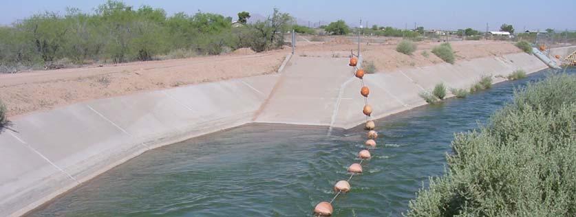
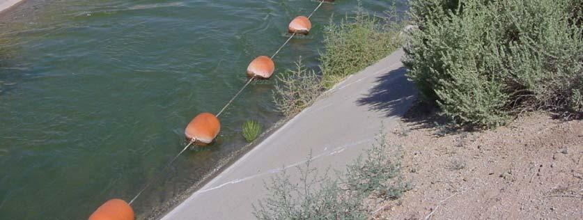
312 Gary P. Merkley 304 BIE 5300/6300 Lectures