3-1. all x all y. [Figure 3.1]

Transcription

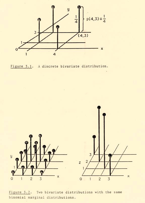
1 - Chapter. Multivariate Distributions. All of the most interesting problems in statistics involve looking at more than a single measurement at a time, at relationships among measurements and comparisons between them. In order to permit us to address such problems, indeed to even formulate them properly, we will need to enlarge our mathematical structure to include multivariate distributions, the probability distributions of pairs of random variables, triplets of random variables, and so forth. We will begin with the simplest such situation, that of pairs of random variables or bivariate distributions, where we will already encounter most of the key ideas.. Discrete Bivariate Distributions. If X and Y are two random variables defined on the same sample space S; that is, defined in reference to the same experiment, so that it is both meaningful and potentially interesting to consider how they may interact or affect one another, we will define their bivariate probability function by p(x, y) P (X x and Y y). (.) In a direct analogy to the case of a single random variable (the univariate case), p(x, y) may be thought of as describing the distribution of a unit mass in the (x, y) plane, with p(x, y) representing the mass assigned to the point (x, y), considered as a spike at (x, y) of height p(x, y). The total for all possible points must be one: p(x, y). (.2) all x all y [Figure.] Example.A. Consider the experiment of tossing a fair coin three times, and then, independently of the first coin, tossing a second fair coin three times. Let X #Heads for the first coin Y #Tails for the second coin Z #Tails for the first coin. The two coins are tossed independently, so for any pair of possible values (x, y) of X and Y we have, if {X x} stands for the event X x, p(x, y) P (X x and Y y) P ({X x} {Y y}) P ({X x}) P ({Y y}) P X (x) P Y (y). On the other hand, X and Z refer to the same coin, and so p(x, z) P (X x and Z z) P ({X x} {Z z}) P ({X x}) p X (x) if z x otherwise. This is because we must necessarily have x + z, which means {X x} and {Z x } describe the same event. If z x, then {X x} and {Z z} are mutually exclusive and the probability both occur

2 -2 is zero. These bivariate distributions can be summarized in the form of tables, whose entries are p(x, y) and p(x, z) respectively: x 2 y x 9 2 p(x, y) p(x, z) Now, if we have specified a bivariate probability function such as p(x, y), we can always deduce the respective univariate distributions from it, by addition: z p X (x) all y p(x, y), (.) p Y (y) p(x, y), (.4) all x The rationale for these formulae is that we can decompose the event {X x} into a collection of smaller sets of outcomes. For example, {X x} {X x and Y } {X x and Y } {X x and Y 2} where the values of y on the righthand side run through all possible values of Y. But then the events of the righthand side are mutually exclusive (Y cannot have two values at once), so the probability of the righthand side is the sum of the events probabilities, or p(x, y), while the lefthand side has probability p X (x). all y When we refer to these univariate distributions in a multivariate context, we shall call them the marginal probability functions of X and Y. This name comes from the fact that when the addition in (.) or (.4) is performed upon a bivariate distribution p(x, y) written in tabular form, the results are most naturally written in the margins of the table. Example.A (continued). For our coin example, we have the marginal distributions of X, Y, and Z: x 2 P y (y) y 2 p X (x) 2 p X (x) x 2 p z (z) This example highlights an important fact: you can always find the marginal distributions from the bivariate distribution, but in general you cannot go the other way: you cannot reconstruct the interior of a table (the bivariate distribution) knowing only the marginal totals. In this example, both tables have exactly the same marginal totals, in fact X, Y, and Z all have the same Binomial (, 2) distribution, but z

3 - the bivariate distributions are quite different. The marginal distributions p X (x) and p Y (y) may describe our uncertainty about the possible values, respectively, of X considered separately, without regard to whether or not Y is even observed, and of Y considered separately, without regard to whether or not X is even observed. But they cannot tell us about the relationship between X and Y, they alone cannot tell us whether X and Y refer to the same coin or to different coins. However, the example also gives a hint as to just what sort of information is needed to build up a bivariate distribution from component parts. In one case the knowledge that the two coins were independent gave us p(x, y) p X (x) p Y (y); in the other case the complete dependence of Z on X gave us p(x, z) p X (x) or as z x or not. What was needed was information about how the knowledge of one random variable s outcome may affect the other: conditional information. We formalize this as a conditional probability function, defined by p(y x) P (Y y X x), (.5) which we read as the probability that Y y given that X x. Since Y y and X x are events, this is just our earlier notion of conditional probability re-expressed for discrete random variables, and from (.7) we have that as long as p X (x) >, with p(y x) undefined for any x with p X (x). p(y x) P (Y y X x) (.6) P (X x and Y y) P (X x) p(x, y) p X (x), If p(y x) p Y (y) for all possible pairs of values (x, y) for which p(y x) is defined, we say X and Y are independent variables. From (.6), we would equivalently have that X and Y are independent random variables if p(x, y) p X (x) p Y (y), for all x, y. (.7) Thus X and Y are independent only if all pairs of events X x and Y y are independent; if (.7) should fail to hold for even a single pair (x o, y o ), X and Y would be dependent. In Example.A, X and Y are independent, but X and Z are dependent. For example, for x 2, p(z x) is given by p(z 2) p(2, z) p X (2) if z otherwise, so p(z x) p Z (z) for x 2, z in particular (and for all other values as well). By using (.6) in the form p(x, y) p X (x)p(y x) for all x, y, (.) it is possible to construct a bivariate distribution from two components: either marginal distribution and the conditional distribution of the other variable given the one whose marginal distribution is specified. Thus while marginal distributions are themselves insufficient to build a bivariate distribution, the conditional probability function captures exactly what additional information is needed.

4 .2 Continuous Bivariate Distributions. -4 The distribution of a pair of continuous random variables X and Y defined on the same sample space (that is, in reference to the same experiment) is given formally by an extension of the device used in the univariate case, a density function. If we think of the pair (X, Y ) as a random point in the plane, the bivariate probability density function f(x, y) describes a surface in -dimensional space, and the probability that (X, Y ) falls in a region in the plane is given by the volume over that region and under the surface f(x, y). Since volumes are given as double integrals, the rectangular region with a < X < b and c < Y < d has probability P (a < X < b and c < Y < d) [Figure.] It will necessarily be true of any bivariate density that and d b c a f(x, y)dxdy. (.9) f(x, y) for all x, y (.) f(x, y)dxdy, (.) that is, the total volume between the surface f(x, y) and the x y plane is. Also, any function f(x, y) satisfying (.) and (.) describes a continuous bivariate probability distribution. It can help the intuition to think of a continuous bivariate distribution as a unit mass resting squarely on the plane, not concentrated as spikes at a few separated points, as in the discrete case. It is as if the mass is made of a homogeneous substance, and the function f(x, y) describes the upper surface of the mass. If we are given a bivariate probability density f(x, y), then we can, as in the discrete case, calculate the marginal probability densities of X and of Y ; they are given by f X (x) f Y (y) f(x, y)dy for all x, (.2) f(x, y)dx for all y. (.) Just as in the discrete case, these give the probability densities of X and Y considered separately, as continuous univariate random variables. The relationships (.2) and (.) are rather close analogues to the formulae for the discrete case, (.) and (.4). They may be justified as follows: for any a < b, the events a < X b and a < X b and < Y < are in fact two ways of describing the same event. The second of these has probability b a f(x, y)dxdy b a b a f(x, y)dydx [ ] f(x, y)dy dx. We must therefore have P (a < X b) b a [ ] f(x, y)dy dx for all a < b, and thus f(x, y)dy fulfills the definition of f X(x) (given in Section.7): it is a function of x that gives the probabilities of intervals as areas, by integration.

5 -5 In terms of the mass interpretation of bivariate densities, (.2) amounts to looking at the mass from the side, in a direction parallel to the y axis. The integral x+dx x [ ] f(u, y)dy du f(x, y)dy dx gives the total mass (for the entire range of y) between x and x + dx, and so, just as in the univariate case, the integrand f(x, y)dy gives the density of the mass at x. Example.B. Consider the bivariate density function ( ) f(x, y) y 2 x + x for < x <, < y < 2 otherwise. One way of visualizing such a function is to look at cross-sections: the function f ( ( x, 2) 2 2 x) + x x is the cross-section of the surface, cutting it with a plane at y 2. [Figure.4] We can check that f(x, y) is in fact a bivariate density, by evaluating its double integral in an iterated form, taking account of the fact that f(x, y) vanishes outside of the rectangle < x <, < y < 2: f(x, y)dxdy { [ ( ) y 2 x [ ( ) y 2 x ( ) y 2 x dx + ( ) 2 x dx + [ [ y [ y + 2 In the process of evaluating this double integral, we found f(x, y)dx ] dy 2 dy 2 2. ] + x dxdy ] } + x dx dy [ ( ) ] y 2 x + x dx ] xdx dy ] xdx dy 2 for all < y < 2; that is, the marginal density of Y is f Y (y) 2 for < y < 2 otherwise.

6 We recognize this as the Uniform (, 2) distribution. We could also calculate f X (x) 2 f(x, y)dy -6 [ ( ) ] y 2 x + x dy for < x < ( ) 2 2 x ydy + 2x for < x < ( ) 2 2 x + 2x for < x < for < x < otherwise. This is just the Uniform (, ) distribution! Now if the events a < X < b and c < Y < d were independent for all a, b, c, d, we would be able to express P (a < X < b and c < Y < d) in terms of these marginal densities: P (a < X < b and c < Y < d) P (a < X < b) P (c < Y < d) b a b d a f X (x)dx c d c f Y (y)dy f X (x)f Y (y)dydx, and thus the product f X (x)f Y (y) would fulfil the role of the bivariate density f(x, y). But in this example, f X (x)f Y (y) 2 f(x, y); evidently the events in question are not independent in this example. This example highlights the fact that, just as in the discrete case, we cannot construct a bivariate density from univariate marginal densities, even though we can go the other way and find the marginal densities from the bivariate density. We cannot reconstruct the entire surface f(x, y) from two side views, f X (x) and f Y (y). More information is needed; that information is given by the conditional densities.. Conditional Probability Densities. In the discrete case we defined the conditional distribution of Y given X as p(y x) p(x, y) p X (x), if p X(x) >. (.6) We shall follow an analogous course and define the conditional probability density of a continuous random variable Y given a continuous random variable X as f(y x) f(x, y) f X (x), if f X(x) >, (.4) and leave the density f(y x) undefined if f X (x). The parallel between (.6) and (.4) can be helpful, but it is deceptive. The relationship (.6) is as we noted, nothing more than a re-expression of our original definition of conditional probability P (E F ) P (E F ) (.7) P (F ) for the special case E Y y and F X x. On the other hand, the definition (.4) represents a significant extension of (.7). The reason is that it represents the distribution of Y given X x, but, as

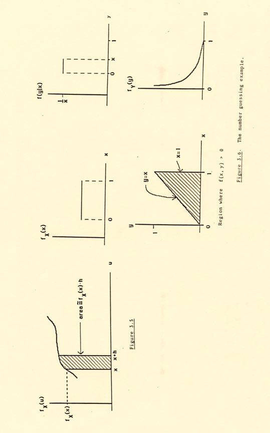
7 -7 we saw in Section.7, for a continuous random variable X we must have P (X x) for each x, and we have not yet defined conditional probabilities where the given event has probability zero. The rationale for the definition (.4) can best be presented by starting with the use to which f(y x) will be put. For f(y x) is a density, and it will give conditional probabilities as areas, by integration. In particular, we will have P (a < Y b X x) b a f(y x)dy for all a < b. (.5) (Indeed, an alternative mathematical approach would start with (.5) and deduce (.4)). But what does P (a < Y b X x) mean, since P (X x) and (.7) does not apply? We proceed heuristically. By P (a < Y b X x) we surely must mean something very close to P (a < Y b x X x + h) for h very small. If f X (x) >, this latter probability is well-defined, since P (x X x + h) >, even though it may be quite small. But then, P (a < Y b X x) P (a < Y b x X x + h) P (x X x + h and a < Y b) P (x X x + h) [ b ] x+h f(u, y)du dy a x x+h. f x X (u)du But if the function f X (u) does not change value greatly for u in the small interval [x, x + h], we have approximately, x+h x f X (u)du f X (x) h [Figure.5]. Similarly, if for fixed y the function f(u, y) does not change value greatly for u in the small interval [x, x+h], we have, again approximately, x+h x f(u, y)du f(x, y) h. Substituting these approximations into the above expression gives P (a < Y b X x) b a b a b a f(x, y) hdy f X (x) h f(x, y)dy f X (x) [ ] f(x, y) dy. f X (x) Comparing this with (.5) gives us (.4). This is not a mathematically rigorous demonstration that (.4) is the proper definition of conditional density, but it captures the essence of one possible rigorous approach, which would combine the passage to the limit of h with ideas from measure theory. An intuitive interpretation of conditional densities in terms of the bivariate density is easy: f(y x) is just the cross-section of the surface f(x, y) at X x, rescaled so that it has total area. Indeed, for a fixed x, f X (x) in the denominator of (.4) is just the right scaling factor so that the area is : [ ] f(x, y) f(y x)dy dy f X (x) f X (x) f(x, y)dy f X (x) f X(x) from (.2) for any x with f X (x) >.

8 Example.B (Continued). The conditional density of X given Y y, if < y < 2, is f(x y) f(x, y) f Y (y) - y ( 2 x) + x for < x < 2 y( 2x) + 2x for < x < otherwise. This is, except for the scaling factor /2, just the equation for the cross-sections shown in Figure.4. For y /2, we have ( f x ) x + for < x < 2 2 otherwise. We note that these cross-sections, which we now interpret as unscaled conditional densities, vary with y in shape as well as scale. In general, if f(y x) f Y (y) for all y, all x with f X (x) > (.6) or equivalently or equivalently f(x y) f X (x) for all x, all y with f Y (y) > (.7) f(x, y) f X (x) f Y (y) for all x and y (.) we shall say that X and Y are independent random variables. Any one of these conditions is equivalent to P (a < X < b and c < Y < d) P (a < X < b) P (c < Y < d) (.9) for all a, b, c, d. If any one of these conditions fails to hold, X and Y are dependent. As we have observed, in Example.B X and Y are dependent random variables. In general, by turning (.4) around, one marginal density (say of X) and one set of conditional densities (say those of Y given X) determine the bivariate density by f(x, y) f X (x)f(y x) for all x, y. (.2) Example.C. Suppose I choose a number X between and at random, and then you peek at my number and choose a smaller one Y, also at random. If the object of the game is to choose the smallest number, then clearly you will win. But by how much? What is the expectation of your choice, Y? What is the distribution of Y? All of these questions require that we be specific about what at random means. Suppose we take it to be uniformly distributed, so I choose according to a Uniform (, ) distribution f X (x) for < x < otherwise, and, conditional on your observing my X x, you choose according to a Uniform (, x) distribution, f(y x) x for < y < x otherwise.

9 -9 Now from (.2) we have f(x, y) f X (x)f(y x) x for < x < and < y < x otherwise. The bivariate density of X and Y is thus positive over a triangle. [Figure.6] Once we have found the bivariate density of X and Y, we can proceed with our calculations. marginal density of Y (that is, the univariate density of Y, ignoring X) is found to be f Y (y) y f(x, y)dx x dx log e (x) y The log e (y) for < y < otherwise. Notice that in performing this calculation it was particularly important to keep track of the range over which the density is positive. For a particular y, f(x, y) /x only for < y < x and < x <, so since both of these conditions must be met we have y < x < as the range of integration. The marginal density of Y piles up mass near, reflecting the fact that Y has been selected as smaller than some value of X. One of the questions asked was, what is the expectation of Y? There is a bit of ambiguity here, does it refer to the marginal distribution of Y, in which the value of X is ignored in making the calculation? Or does it refer to the conditional expectation of Y, given the value of X x? Because no reference is made to given X x, it is perhaps most natural to calculate the marginal expectation of Y, E(Y ) 4 yf Y (y)dy y log e (y)dy 4 Γ(2) 4. ze z dz (by change -of-variable; z 2 log e y, dy e z 2 dz) (We will see an easier way of finding E(Y ) later.) Thus, since E(X) x dx 2, the marginal expected value of the smaller number is just half that of X. We can also evaluate the conditional expectation of Y given X x; it is just the expectation of the conditional distribution f(y x), E(Y X x) x yf(y x)dy y x dy x x2 2 x 2,

10 - a result that is obvious since E(Y X x) must be the center of gravity of f(y x) (see Figure.6). So either marginally or conditionally, the second choice is expected to be half the first. What about the other question what is the expected amount by which Y is less than X, E(X Y )? This requires further development of the mathematics of expectation..4 Expectations of Transformations of Bivariate Random Variables. A transformation of a bivariate random variable (X, Y ) is, as in the univariate case, another random variable that is defined as a function of the pair (X, Y ). For example, h (X, Y ) X + Y, h 2 (X, Y ) X Y, and h (X, Y ) X Y are all transformations of the pair (X, Y ). We can find the expectation of a transformation h(x, Y ) in principle by noting that Z h(x, Y ) is a random variable, and if we can find the distribution of Z, its expectation will follow: E(Z) all z zp Z (z) in the discrete case or E(Z) zf Z (z)dz in the continuous case. General techniques for finding the distribution of transformations h(x, Y ) are generalizations of those used for the univariate case in Section.. But it will turn out that they are unnecesasary in most cases, that we can find Eh(X, Y ) without going through the intermediate step of finding the distribution of h(x, Y ), just as was the case for univariate transformations (Section 2.2). For by a generalized change-of-variables argument, it can be established that Eh(X, Y ) h(x, y)p(x, y) in the discrete case, (.2) all x all y Eh(X, Y ) h(x, y)f(x, y)dxdy in the continuous case. (.22) These formulae will hold as long as the expressions they give do not diverge; h need not be monotone or continuous. Example.C (Continued). We had asked earlier for the expectation of X Y, the amount by which the first choice exceeds the second. Here we have h(x, Y ) X Y, and E(X Y ) y (x y)f(x, y)dxdy (x y) x dxdy [ x y x dx [ dx y y y y x dx [( y) + y log e (y)] dy ( y)dy , y ] x dx dy ] dy y log e (y)dy

11 - where we used the fact that we earlier evaluated y log e(y)dy /4. (We may note that here E(X Y ) E(X) E(Y ); we shall later see that this is always true.) We could also calculate the expectation of h(x, Y ) XY, E(XY ) xy y x dxdy [ ] ydx dy y [ y y ] dx dy y( y)dy 6. Notice that E(X)E(Y ) /2 /4 /; we do not have E(XY ) E(X)E(Y ). We shall later see that this reflects the fact that X and Y are not independent. Earlier we calculated E(Y ) for this example, a result that depended upon a change-of-variable and recognizing the result as a Gamma function. Here is a simpler alternative route to the same end, based upon treating Y as a special case of a transformation of (X, Y ): h(x, Y ) Y. Then E(Y ) y x x y x dxdy y x dydx [ x ] ydy dx x x2 2 dx x 2 dx 4. (We shall see an even simpler calculation later, in Section.!).5 Mixed Cases. (reversing the order of integration) We have encountered bivariate distributions with both X and Y discrete, and with both X and Y continuous. It is not a long step further to consider situations in which X is discrete and Y is continuous. Example.D. Bayes s Billiard Table. Perhaps the earliest such example was one presented in a famous article published in the Philosophical Transactions of the Royal Society of London in 7, by the Reverend Thomas Bayes. Imagine a flat rectangular table (we might call it a billiard table) with a scale marked on one side, from to. A ball is rolled so that it may be considered to be equally likely to come to rest at any point on the table; its final position, Y, is marked on the scale on the side. [Figure.7] A second ball is then rolled n times, and a count is made of the number of times X it comes to rest to the left of the marked position Y. Then (X, Y ) is a bivariate random variable, and X is discrete and Y is continuous. From the description of the experiment, Y has a Uniform (, ) distribution, with density f Y (y) < y < otherwise.

12 -2 If we consider each subsequent role as being made independently, then conditional upon Y y, X is a count of the number of successes in n Bernoulli trials where the chance of success on a single trial is y. That is, the conditional distribution of X given Y y is Binomial (n, y): p(x y) ( n x ) y x ( y) n x otherwise. for x,,..., n For mixed cases as for other cases, we can construct the bivariate distribution by multiplication: f(x, y) f Y (y) p(x y) (.2) ( n ) y x ( y) n x for y and x,, 2,..., n, x otherwise. This distribution is a hybrid; it is discrete in the argument x and continuous in the argument y. It might be pictured as a series of parallel sheets resting on the x y plane, concentrated on the lines x, x,..., x n. For example, the cross-section at x is the sheet whose upper edge has the outline described, as a function of y, by f(, y) ny( y) n y [Figure.] The cross-section parallel to the x-axis at a particular value of y shows the spikes of the Binomial (n, y) distribution. For dealing with mixed cases, we can use our results for the discrete and continuous cases. For example, the (discrete) marginal distribution of X is p X (x) f(x, y)dy (.24) ( n x ) y x ( y) n x dy ( n ) y x ( y) n x dy x ( n ) B(x +, n x + ) (from (2.2)) x ( n ) ) x (n + ) ( n x for x,, 2,..., n, n + otherwise. (We evaluated the integral by recognizing it was a Beta function (2.2), and by using the identity given just before (2.2), where the reciprocal of the Beta function is given for integer arguments.) We recognize the result as the discrete uniform distribution of Example 2.. An observer of this experiment who was not in a position to note the value of Y, but would only learn the count X, would find all possible values of X equally likely. We can also calculate the conditional distribution of Y given X x. For x,,..., n it will be a density, given by f(y x) f(x, y) p X (x) (.25)

13 - ( n ) x y x ( y) n x ( ) (n + ) n+ otherwise. ( n x ) y x ( y) n x for y (If x is not an integer, p X (x) and f(y x) is undefined.) We can recognize this as a Beta density, with α x + and β n x +. We shall discuss the potential uses of these calculations for statistical inference in the next chapter..6 Higher Dimensions. We have concentrated on bivariate distributions because of their mathematical simplicity, and because they are easier to visualize than higher dimensional distributions are. The same ideas carry over to higher dimensions, however. If X, X 2, and X are three discrete random variables, their trivariate distribution is described by a probability function and p(x, x 2, x ) P (X x and X 2 x 2 and X x ), all x, x 2, x p(x, x 2, x ). If X, X 2, and X are continuous, we would describe their distribution by a density f(x, x 2, x ), where f(x, x 2, x )dx dx 2 dx, and the same integral over a restricted range in X, X 2, X, space would give the probability the random point (X, X 2, X ), falls in that restricted range. More general multivariate distributions and would be defined analogously. p(x, x 2,..., x n ) f(x, x 2,..., x n ) We will say a collection of random variables are independent if their multivariate distribution factors into a product of the univariate distributions for all values of the arguments: in the discrete case, in the continuous case, p(x, x 2,..., x n ) p X (x )p X2 (x 2 ) p Xn (x n ); (.26) f(x, x 2,..., x n ) f X (x )f X2 (x 2 ) f Xn (x n ). (.27) The terms on the right here are the marginal distributions of the X i s. They can be found here, as in the bivariate case, by summation or integration. For example, in the trivariate case p X (x ) all x 2, x p(x, x 2, x ); or f X (x ) f(x, x 2, x )dx 2 dx.

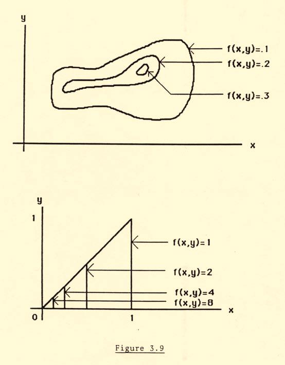
14 -4 We may also have multivariate marginal distributions: If X, X 2, X, and X 4 dimensional distribution, the marginal density of (X, X 2 ) is have a continuous four f(x, x 2 ) f(x, x 2, x, x 4 )dx dx 4. Conditional distributions can be found in a manner analogous to that in the bivariate case. For example, the conditional bivariate density of X and X 4 given X x and X 2 x 2 is f(x, x 4 x, x 2 ) f(x, x 2, x, x 4 ). f(x, x 2 ) Expectations of transformations are found in the same way: in the discrete case, E(h(X, X 2,..., X n )) h(x, dx 2,..., x n )p(x, x 2,..., x n ), (.2) all x s in the continuous case, E(h(X, X 2,..., X n ))... h(x,..., x n )f(x,..., x n )dx,..., dx n. (.29) Mathematically, the problems that arise in higher dimensions can be quite intricate, though they will be considerably simplified in many of the cases we will consider by the fact that the random variables will be specified to be independent..7 Measuring Multivariate Distributions. Describing multivariate distributions can be a complicated task. The entire distribution can be given by the probability function or probability density function, but such a description can be hard to visualize. Univariate distributions can often be better understood by graphing them, but this becomes more difficult with multivariate distributions: the distribution of a trivariate random variable requires a four dimensional picture. Graphs of marginal distributions can help, but as we have emphasized, it is only under additional assumptions (such as independence) that the marginal distributions tell the whole story. In the bivariate case, we could use, for example, the fact that f(x, y) f X (x)f(y x), and graph f(y x) as a function of y for a selection of values of x, together with a graph of f X (x). This would effectively show the surface by showing cross-sections (the f(y x) s) and a side view (f X (x)). In the bivariate case we could also show the surface by plotting level curves; that is, through contour plots of the type used in geography to show three dimensions in two. [Figure.9] This is tantamount to slicing the surface f(x, y) parallel to the x y plane at various heights and graphing the cross-sections on one set of axes. Even though with special computer technology these graphical devices are becoming increasingly popular, and some can in limited ways be adapted to higher dimensions, we will have frequent need for numerical summary measures which, while they do not describe the entire distribution, at least capture some statistically important aspects of it. The measures we consider here are based upon expectations of transformations of the multivariate random variable, such as Eh(X, Y ). A natural starting point for multivariate summary measures is linear transformations; in the bivariate case, h(x, Y ) ax + by, where a and b are constants.

15 -5 The following theorem shows that the expectations of linear transformations are particularly easy to evaluate: Theorem: For any constants a and b and any multivariate random variable (X, Y ), as long as all of these expressions are well defined. Proof (for the continuous case). From (.22) we have E(aX + by ) a a E(aX + by ) ae(x) + be(y ), (.) (ax + by)f(x, y)dxdy [axf(x, y) + byf(x, y)]dxdy axf(x, y)dxdy + [ x f(x, y)dy xf X (x)dx + b ae(x) + be(y ). ] dx + b byf(x, y)dxdy [ ] y f(x, y)dx dy yf Y (y)dy (using (.2), (.)) (Alternatively, we could have skipped the fourth and fifth steps here by noticing, for example, that (.22) with h(x, y) ax tells us that The proof for the discrete case is similar. axf(x, y)dxdy E(aX) ae(x).) These results can be immediately generalized by induction: For any a, a 2,..., a n and any multivariate random variable (X, X 2,..., X n ), ( n ) E a i X i i n a i E(X i ), (.) as long as all expressions are well-defined (that is, the expectations do not diverge.) This Theorem can be quite helpful; it tells us that it is easy to compute expectations of linear transformations such as ax + by, because all we need to know are the separate marginal distributions of X and Y. But the Theorem has a negative aspect as well: since E(aX + by ) can be determined from facts about the marginal distributions alone for any a and b, in particular from knowing just E(X) and E(Y ), and since the marginal distributions do not allow us to reconstruct the bivariate distribution, it is hopeless to try to capture information about how X and Y vary together by looking at expectations of linear transformations! It is simply impossible for summary measures of the form E(aX + by ) to tell us about the degree of dependence (or lack of it) between X and Y. To learn about how X and Y vary together, we must go beyond expectations of linear transformations. i

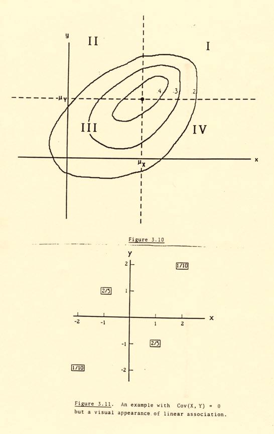
16 -6. Covariance and Correlation. The simplest nonlinear transformation of X and Y is XY, and we could consider E(XY ) as a summary. Because E(XY ) is affected by where the distributions are centered as well as how X and Y vary together, we start instead with the product of X E(X) and Y E(Y ), that is the expectation of This is called the covariance of X and Y, denoted h(x, Y ) (X µ X )(Y µ Y ). Cov(X, Y ) E[(X µ X )(Y µ Y )]. (.2) By expanding h(x, Y ) XY µ X Y Xµ Y + µ X µ Y and using (.) we arrive at an alternative expression, Cov(X, Y ) E(XY ) µ X E(Y ) µ Y E(X) + µ X µ Y E(XY ) µ X µ Y µ Y µ X + µ X µ Y or Cov(X, Y ) E(XY ) µ X µ Y. (.) It is immediate from either (.2) or (.) that Cov(X, Y ) Cov(Y, X). Example.C. (Continued) For the density f(x, y) x for < y < x < otherwise, we found E(X) µ X 2, E(Y ) µ Y 4, and We then have E(XY ) 6. Cov(X, Y ) Note that in view of (.), Covariance may be considered as a measure of exactly how much E(XY ) differs from E(X)E(Y ). But how are we to interpret the magnitude of this measure? To begin with and to help see how it relates qualitatively to the bivariate distribution of X and Y, consider Figure., showing contours for a bivariate distribution. When [Figure.] X and Y are in quadrant I or quadrant III, (X µ x )(Y µ Y ) is positive; in quadrants II and IV (X µ X )(Y µ Y ) is negative. If there is a tendency for (X, Y ) to be in I or III, as in Figure., we would expect positive values to dominate and Cov(X, Y ) > ; covariance is, after all, a weighted average value of (X µ X )(Y µ Y ), weighted by the probabilities of the different values of this product.

17 -7 Qualitatively, a positive Cov(X, Y ) suggests that large values of X are associated with large values of Y, and small values of X are associated with small values of Y. At one extreme, if X and Y are the same random variable, we have Cov(X, X) E(X X) µ X µ X (.4) Var(X). But covariance can be negative as well, if large values of X are associated with small values of Y. The extreme case is Y X, in which case, since µ X µ X, Cov(X, X) E(X( X)) µ X µ X (.5) E(X 2 ) + µ 2 X Var(X). We can think of X Y and X Y as representing extremes of positive and negative dependence, and intermediate between these extremes is the case of independence. If X and Y are independent, To see this, consider E(XY ) µ X µ Y ; Cov(X, Y ). (.6) xyf(x, y)dxdy (.7) xyf X (x)f Y (y)dxdy xf X (x)dx yf Y (y)dy by independence a similar argument gives E(XY ) µ X µ Y in the discrete case. But Cov(X, Y ) is not sufficient to guarantee independence; intuitively there can be an exact balance between the weighted values of h(x, Y ) (X µ X )(Y µ Y ) in quadrants I and III and in quadrants II and IV of Figure. for dependent X and Y. Example.E. Suppose (X, Y ) has the bivariate discrete distribution p(x, y) given by the table y p X (x) x p X (y) Then and so µ X µ Y E(XY ) ( 2)( 2) + ( ) ( ) , Cov(X, Y ).

18 - Yet p(x, y) p X (x)p Y (y) for any possible pair (x, y); X and Y are dependent. [Figure.] In general, we shall refer to two random variables with Cov(X, Y ) as uncorrelated, keeping in mind that they may still be dependent, though the dependence will not be of the monotone sort exhibited in Figure.. The most important single general use of covariance, and the best means of interpreting it quantitatively, is by viewing it as a correction term that arises in calculating the variance of sums. By using (.) with a b, we have already that E(X + Y ) E(X) + E(Y ) (.) (or µ X+Y µ X + µ Y ). Now the variance Var(X + Y ) is the expectation of (X + Y µ X+Y ) 2 [X + Y (µ X + µ Y )] 2 by (.) [(X µ X ) + (Y µ Y )] 2 (X µ X ) 2 + (Y µ Y ) 2 + 2(X µ X )(Y µ Y ). Now, using (.) with X (X µ X ) 2, X 2 (Y µ Y ) 2, X (X µ X )(Y µ Y ), a a 2, and a 2, we have Var(X + Y ) Var(X) + Var(Y ) + 2 Cov(X, Y ). (.9) This is true as long as all expressions are well-defined (ie. do not diverge). Comparing (.) and (.9) illustrates the point made earlier: E(X + Y ) depends only on the marginal distributions, but Var(X + Y ) reflects the bivariate behavior through the covariance correction term. In the extreme cases X Y and X Y we have Var(X + X) Var(X) + Var(X) + 2 Cov(X, X) 4 Var(X) (using.4), while Var(X + ( X)) Var(X) + Var( X) + 2 Cov(X, X), from (.5). The first of these agrees with (2.2) with a 2, b ; the second is obvious since X +( X) has zero variance. In the special case where X and Y are independent (or even uncorrelated), Cov(X, Y ) and Var(X + Y ) Var(X) + Var(Y ). (.4) Thus Cov(X, Y ) can be interpreted quantitatively; it is half the correction term that should be applied to the formula for Var(X + Y ) for the independent case. The interpretation of covariance as a correction factor for variances of sums gives meaning to it as a magnitude, but it reveals a shortcoming to Cov(X, Y ) as a measure of dependence: Cov(X, Y ) changes with multiplicative changes in the scales of measurement of X and Y. In fact, since ax + b µ ax+b a(x µ X ) and we have cy + d µ cy +d c(y µ Y ), Cov(aX + b, cy + d) ac Cov(X, Y ) (.4)

19 -9 for all constants a, b, c, d. Large covariance may be due to a high degree of association or dependence between X and Y ; it may also be due to the choice of scales of measurement. To eliminate this scale effect we define the correlation of X and Y to be the covariance of the standardized X and Y, [( ) ( )] X µx Y µy ρ XY E σ X σ Y ( X µx Cov, Y µ ) Y σ X σ Y Cov(X, Y ). σ X σ Y Example.C (Continued) For the bivariate density (.42) f(x, y) x for < y < x < otherwise, we found E(X) 2, E(Y ) 4, and Cov(X, Y ) 24. Furthermore, E(X 2 ) x 2 dx and so E(Y 2 ) x y 2 x dydx x x2 dx ) 2 x 2 dx 9, Var(X) ( 2 2 We then have Var(Y ) 9 ( 4 ρ XY ) If X and Y were independent with the same marginal distributions, we would have Var(X + Y ) Since they are positively correlated, the variance of X + Y will exceed this by or 2 Cov(X, Y ) , Var(X + Y ) 44. It follows immediately from (.4) and (2.2) that as long as ac >, ρ ax+b,cy +d ρ X,Y, (.4)

20 while if ac <, -2 ρ ax+b,cy +d ρ XY. (.44) That is, correlation is a scale-free measure of the bivariate distribution of X and Y. aspects of the dependence of X and Y. If X and Y are independent, It reflects some ρ XY, (.45) but if X and Y are uncorrelated, that is, if ρ XY, it does not follow that X and Y are independent (as Example.E shows). Correlation may be interpreted as a correction term for the variance of the sum of the standardized variables W X µ X, V Y µ Y, σ X σ Y and looking at it from this point of view will tell us its range of possible values. We have Var(W + V ) Var(W ) + Var(V ) + 2ρ XY + + 2ρ XY 2( + ρ XY ). Since we must have Var(W + V ) for any bivariate distribution, it is always true that + ρ XY, or ρ XY. Since this must also apply with Y for Y, we also have ρ X, Y and (.44) implies ρ X, Y ρ X,Y, (.46) so we must also have ρ XY or ρ XY. Together, these give us the range of possible values of ρxy as ρ XY. (.47) We have already encountered the extremes: ρ XX, while ρ X, X. Even though correlation is scale-free, it is extremely limited as a general measure of dependence or association. The existence of examples such as Example.E suggest what is true, that no single number can adequately capture all the potential complexities of a bivariate distribution. We shall see, however, that in the more restricted setting of a multivariate normal distribution, correlation measures the degree of dependence perfectly..9 Covariance in Higher Dimensions. For general bivariate distributions, covariance and correlation are most useful as correction factors for variances of sums, and of limited usefulness as measures of dependence. As we would expect would be the case, measuring dependence in higher dimensions is even more difficult. However, for the limited purpose of calculating variances of sums, bivariate covariance provides the needed correction factor, even in higher dimensions. Suppose (X,..., X n ) is an n dimensional random variable. Then from (.), and µ X+ +X n µ ΣXi ( n ) 2 ( n X i µ ΣXi (X i µ Xi ) i i ) 2 n µ Xi, (.4) i n (X i µ Xi ) 2 + (X i µ Xi )(X j µ Xj ) all i, j i j i

21 -2 Taking expectations (again using.), ( n ) Var X i i Slightly more generally, we also have ( n ) Var a i X i i n Var(X i ) + Cov(X i, X j ). (.49) all i, j i j i n a 2 i Var(X i ) + a i a j Cov(X i, X j ), (.5) all i, j i j i for any constants a, a 2,..., a n. In the special case where the X s are mutually independent (or, even if they are pairwise uncorrelated), the last double sum in each case equals zero, and we have ( n ) Var X i i ( n ) Var a i X i i n Var(X i ). (.5) i n a 2 i Var(X i ). (.52) Thus the double sum in (.49) and (.5) may be considered as a correction term, capturing the total effect of the dependence among the X s as far as the variance of sums is concerned. We shall be particularly interested in the behavior of arithmetic averages of independent random variables X,..., X n, denoted X n X i. (.5) n From (.) and (.52), with a a n /n, E( X) n i Var( X) n 2 i n µ Xi, (.54) i n i σ 2 X i. (.55) If the X s have the same expectations and variances (µ X µ Xn µ; σ X 2 σ 2 X n σ 2 ), we get E( X) µ, (.56) Var( X) σ 2 /n. (.57) For many statistical purposes it is extraordinarily useful to represent higher dimensional random variables in terms of vector-matrix notation. We can write the multivariate random variable (X, X 2,..., X n ) as a column vector, denoted X X 2 X, X n

22 -22 and the expectations of the X i s as another column vector: µ X µ X2 µ X. µ Xn Symbolically, we then have E(X) µ X ; that is, the expectation of a random vector is the vector of expectations of the components. If a is a column vector of constants, a a 2 a, a n then (.) becomes E(a T X) a T E(X) a T µ X, (.5) where a T is the transpose of a, the row vector a T (a a 2 a n ), and a T X n a i X i is the usual matrix product. It is customary to arrange the variances and covariances i of the X i in the form of a square n n matrix called the Covariance matrix, Var(X ) Cov(X, X 2 ) Cov(X, X ) Cov(X, X n ) Cov(X, X 2 ) Var(X 2 ) Cov(X 2 X ) Cov(X 2 X n ) Cov(X) Cov(X, X )..... Cov(X X n ) Var(X n ) (.59) Since Var(X i ) Cov(X i, X i ), the entry in row i and column j is just Cov(X i, X j ). The reason for this arrangement is that it permits many statistical operations to be written quite succinctly. For example, (.52) becomes Var(a T X) a T Cov(X)a. (.6)

23 -2. Conditional Expectation. If (X, Y ) is a bivariate random variable, the entire bivariate distribution can be reconstructed from one marginal distribution, say f X (x), and the other conditional distributions, say f(y x), for all x. Now the conditional distributions f(y x) are a family of distributions, a possibly different distribution for the variable Y for every value of x. The manner in which these distributions vary with x is informative about how X and Y are related, and the distributions f(y x) can be described in part, just as for any univariate distributions, by their expectations and variances. This does not involve the introduction of a new concept, only a new use for our previous concept. Thus we have the conditional expectation of Y given X x defined by, in the discrete case E(Y X x) all y yp(y x), (.6) in the continuous case E(Y X x) yf(y x)dy. (.62) Other expectations can be found by application of results previously discussed; for example, for the continuous case E(h(Y ) X x) h(y)f(y x)dy. (.62) This can be applied to define the conditional variance of Y given X x by, in the discrete case, Var(Y X x) all y(y E(Y X x)) 2 p(y x), (.6) and in the continuous case, Var(Y X x) (y E(Y X x)) 2 f(y x)dy. (.) Note that Var(Y X x) E(Y 2 X x) [E(Y X x)] 2 follows from (2.26). Now, as emphasized above, E(Y X x) and Var(Y X x) are, despite the new names, only ordinary expectations and variances for the univariate distributions p(y x) or f(y x). However, there are many of them, one E(Y X x) and one Var(Y X x) for each possible value of X. Indeed, looked at this way, they are transformations of X, just as h(x) X 2 or h(x) X + 2 are transformations of X. Thus if we consider X as a random variable, these particular transformations of X may be considered as random variables. Viewed this way, we will write E(Y X) and mean the random variable which, when X x, takes the value E(Y X x). Similarly, Var(Y X) is a random variable that equals Var(Y X x) when X x. Furthermore, as the random variables with univariate probability distributions, we can discuss the expectation and variance of E(Y X) and Var(Y X). Now, in practice it may be quite difficult to actually determine the distributions of E(Y X) and Var(Y X), but two identities involving their expectations, play a remarkable role in statistical theory, as we shall see later. These are given in the following theorem. Theorem: For any bivariate random variable (X, Y ), E[E(Y X)] E(Y ), (.65) Var(Y ) E(Var(Y X)) + Var(E(Y X)). (.66) (The first of these has been called Adam s Theorem, because for every claimed first use, someone has found an earlier use.)

24 -24 Proof: (for the continuous case). The expression E[E(Y X)] simply means E(h(X)), for the h(x) given by (.62). We have [ ] E[E(Y X)] yf(y x)dy f X (x)dx E(Y ), using (.22) with h(x, y) y. For the second result, using (.65) with Y 2 for Y. Also, yf(y x)f X (x)dydx yf(x, y)dydx E(Var(Y X)) E{E(Y 2 X) [E(Y X)] 2 } E[E(Y 2 X)] E[E(Y X)] 2 E(Y 2 ) E[E(Y X)] 2, Var(E(Y X)) E[E(Y X)] 2 {E[E(Y X)]} 2 E[E(Y X)] 2 [E(Y )] 2 using (.65) directly. Adding these two expressions gives the result (.66), since two terms cancel to give E(Y 2 ) [E(Y )] 2 Var(Y ). Example.C (Continued). Here the distribution of X is Uniform (, ) and that of Y given X x is Uniform (, x). Now it is immediate that the expectation of a Uniform random variable is just the midpoint of its range: E(Y X x) x 2 for < x <. Then E(Y X) is the random variable X/2. But E(X) /2. so E(Y ) E(E(Y X)) E(X/2) E(X)/2 4. The first time we found this result, it involved evaluating the difficult integral y log e(y)dy, the second time we found it from evaluting a double integral. Continuing, the variance of a Uniform (, x) distribution is x 2 /2. We have Var(Y ) E(Var(Y X)) + Var(E(Y X)) E(X 2 /2) + Var(X/2) E(X 2 )/2 + Var(X)/

25 -25. Application: Binomial Distribution. In Chapter we encountered the Binomial (n, θ) Distribution, the distribution of the discrete univariate random variable X, ( n ) b(x; n, θ) θ x ( θ) n x for x,, 2,..., n x otherwise. It is possible to evaluate E(X) and Var(X) directly from the definitions, with some cleverness. Paradoxically, it is much easier to evaluate them by considering X as a transformation of a multivariate random variable. The random variable X is the total number of successes in n independent trials. Let X i be the number of successes on the i th trial; that is, X i if i th trial is a success if i th trial is a failure. Then (X, X 2,..., X n ) is a multivariate random variable of a particularly simple kind, and all the X i s are mutually independent. Furthermore, n X X i. i Now E(X i ) θ + ( θ) θ, E(X 2 i ) 2 θ + 2 ( θ) θ, and Var(X i ) θ θ 2 θ( θ). From (.4) and (.5) we have E(X) Var(X) n E(X i ) (.67) i n θ nθ, i n Var(X i ) (.6) i nθ( θ). With these basic formulae, let us take another look at Bayes s Billiard Table (Example.D). There we had Y as a continuous random variable with a Uniform (, ) distribution, and, given Y y, X had a Binomial (n, y) distribution. We found that the marginal distribution of X was a discrete uniform distribution, p X (x) for,,..., n n + otherwise. We have just established that E(X Y y) ny, Var(X Y y) ny( y).

26 -26 Thus E(X Y ) and Var(X Y ) are the continuous random variables ny and ny ( Y ) respectively. From (.65) and (.66) we have E(X) E[E(X Y )] E(nY ) n E(Y ) n 2, Var(X) E(Var(X Y )) + Var(E(X Y )) E(nY ( Y )) + Var(nY ) ne(y ) ne(y 2 ) + n 2 Var(Y ) n 2 n + n2 2 These agree with the results found in Example 2.. n(n + 2). 2

27

28

29

30

31

32