Ch3. TRENDS. Time Series Analysis

Transcription

1

2 3.1 Deterministic Versus Stochastic Trends The simulated random walk in Exhibit 2.1 shows a upward trend. However, it is caused by a strong correlation between the series at nearby time points. The true process is Y t = Y t 1 + e t or Y t = t i=1 e t, which has zero mean and increasing variance over time. We call such a trend a stochastic trend. By comparison, the average monthly temperature series in Exhibit 1.7 shows a cyclical trend. We may model it by Y t = µ t + X t, where µ t is a deterministic function with period 12 (µ t = µ t 12 ), and X t is a zero mean unobserved variation (or noise). We say that this model has a deterministic trend.

3 3.2 Estimation of a Constant Mean Consider a model with a constant mean function Y t = µ + X t, E(X t ) = 0. The most common estimate of µ is the sample mean Y = 1 n Y t. Then E(Y ) = µ. So Y is a unbiased estimator n t=1 of µ. If {Y t } is stationary with acf ρ k, Ex 2.17 shows that [ VarY = γ n 1 ( k ) ] ρ k. (1) n n k=1 For many stationary processes, the acf decays quickly that ρ k <. Under this assumption, we have k=0 VarY γ 0 n [ k= ρ k ] for large n.

4 So for many stationary processes {Y t }, the variance of Y is inversely proportional to n. Increasing n will improve the estimation. Ex. We use (1) to investigate Y : 1 If {X t } is white noise, then ρ k = 0 for k > 0. So VarY = γ 0 n. 2 If ρ 1 0 but ρ k = 0 for k > 1, then VarY γ 0 n (1 + 2ρ 1 ) as n. 3 If {Y t } is a MA(1) model: Y t = e t + θe t 1, then ρ 1 = θ 1 + θ 2 and ρ k = 0 for k > 1. We have VarY = γ 0 n [ 1 + 2θ 1 + θ 2 ( )] n 1 n (1 + θ)2 1 + θ 2 γ 0 n. When 1 < θ < 0, say θ = 0.5, VarY 0.2γ 0 n. Comparing with the white noise, the negative correlation ρ 1 improves the estimation significantly. When 0 < θ < 1, say θ = +0.5, VarY 1.8γ 0. The positive n correlation ρ 1 reduces the accuracy of estimation.

5 Ex. For an order one autoregressive process Y t = φy t 1 + e t, 1 < φ < 1, we can show that ρ k = φ k for all k. Then [ VarY γ ] 0 φ k (1 + φ) γ 0 = n (1 φ) n. We plot in R the function k= (1 + φ) (1 φ) phi=seq(-.95,.95,0.05) factor=(1+phi)/(1-phi) plot(y=factor,x=phi,type= l ) abline(h=1,col= red ) for 1 < φ < 1: When φ 1, the variance of Y dramatically increases. In fact, φ = 1 is the nonstationary random walk process Y t = Y t 1 + e t. The variance of Y can be very different for a nonstationary process.

6 3.3 Regression Methods We use classical regression analysis to estimate the parameters in the nonconstant mean trend models Y t = µ t + X t, where µ t is deterministic and E(X t ) = 0. These include linear, quadratic, seasonal means, and cosine trends Linear and Quadratic Trends: The deterministic trend linear model is the most widely used model: µ t = β 0 + β 1 t we call β 0 the intercept, and β 1 the slope, resp. The classical least squares regression is to find ˆβ 0 and ˆβ 1 to minimize Q(β 0, β 1 ) = [Y t (β 0 + β 1 t)] 2. t=1 Use partial derivatives to solve that (formulas are not required): n t=1 ˆβ 1 = (Y t Y )(t t) n t=1 (t, ˆβ0 = Y ˆβ 1 t, where t = n + 1 t)2 2.

7 Exhibit. SCL in the Capital Asset Pricing Model (CAPM)

8 The function lm fits a linear model (a regression model) with its first argument being a formula, i.e., an expression including a tilde sign ( ), the left-hand side of which is the response variable and the right-hand side are the covariates or explanatory variables (separated by plus signs if there are two or more covariates). The intercept term can be removed by adding the term -1 on the right-hand side of the tilde sign. The covariates must be separated with a plus sign (+).

9 The function abline is a low-level graphics function. If a fitted simple regression model is passed to it, it adds the fitted straight line to an existing graph. Any straight line of the form y = β 0 + β 1 x can be superimposed on the graph by running the command abline(a=beta0,b=beta1)

10

11 3.3.2 Cyclical or Seasonal Trends Suppose that a seasonal trend, such as the average monthly temperature data in Exhibit 1.7, can be modeled as Y t = µ t + X t, E(X t ) = 0 for all t. One suitable model may be a seasonal mean model, where there are 12 constants (parameters), β 1, β 2,, β 12, giving the expected average temperature for each of the 12 months, such that β 1 t = 1, 13, 25, β 2 t = 2, 14, 26, µ t =. β 12 t = 12, 24, 36,

12 chap3.r: Exhibit 3.3 Regression Results for the Seasonal Means Model Exhibit 3.4 Results for Seasonal Means Model with an Intercept

13 R: The expression season(tempdub) outputs the monthly index of tempdub as a factor, and saves it into the object month.. A factor is a kind of data structure for handling qualitative (nominal) data that do not have a natural ordering like numbers do. However, for purposes of summary and graphics, the user may supply the levels argument to indicate an ordering among the factor values. See TS-ch3.R

14 Exhibit. We may analyze a data set Monthly milk production: pounds per cow. Jan 62 - Dec 75 (Source: Time Series Data Library (citing: Cryer (1986))) imported from Save it as milk.csv, and analyze by the R codes in TS-ch3.R. See TS-ch3.R The model milk.m2 is a combination of linear model with seasonal mean model. We may decompose a time series into a sum or product of trend, seasonal, and stochastic components by decompose command. See TS-ch3.R

15 3.3.3 Cosine Trends: In some cases, seasonal trends can be modeled economically with cosine curves (that incorporate the smooth change expected from one time period to the next while still preserving the seasonality.) The simplest such model is Y t = µ t + X t with µ t = β 0 + β cos(2πft + Φ) = β 0 + β 1 cos(2πft) + β 2 sin(2πft) where β 1 = β cos Φ and β 2 = β sin Φ. We call β(> 0) the amplitude, f the frequency, and Φ the phase of the curve. 1/f is called the period of the cosine wave.

16 Exhibit 3.5 Cosine Trend Model for Temperature Series (chap3.r) Exhibit 3.6 Cosine Trend for the Temperature Series (chap3.r) The harmonic function will return a matrix of the values of cos(2πt) and sin(2πt). See TS-ch3.R for some basic commands of matrix

17 3.4 Reliability and Efficiency of Regression Estimates Reliability and efficiency of estimates lie on the variances of the estimates. Let us analyze the raliability of estimates for some deterministic trends. Assumption: the series is represented as Y t = µ t + X t, where 1 µ t is a deterministic trend of the kind linear, seasonal means, or cosine curves, and 2 {X t } is a zero-mean stationary process with autocovariance and autocorrelation functions γ k and ρ k, respectively. Parameters in a linear model are estimated according to ordinary least squares regression.

18 3.4.1 The seasonal means For N complete years of monthly data, the estimate for the mean for the jth month is By (1), Var ˆβ j = γ 0 N [ N 1 k=1 ˆβ j = 1 N N 1 i=0 Y j+12i ( 1 k N ρ 12k) ], for j = 1, 2,, 12. Only the seasonal autocorrelations, ρ 12, ρ 24,, enter into the above equation. If {X t } is white noise, then Var ˆβ j = γ 0 N. (2)

19 3.4.2 The cosine trends µ t = β 0 + β 1 cos(2πft) + β 2 sin(2πft) For any frequency of the form f = m/n, where m is an integer satisfying 1 m < n/2, the estimates ˆβ 1 and ˆβ 2 are ˆβ 1 = 2 n n t=1 [ cos ( 2πmt n ) Y t ], ˆβ 2 = 2 n n t=1 [ sin ( 2πmt n ) Y t ], (3) Because these are linear functions of {Y t }, their variances can be computed by (1). 1 If {X t } is white noise, we get Var ˆβ 1 = Var ˆβ 2 = 2γ 0 /n. 2 If m/n = 1/12 and ρ k = 0 for k > 1, then Var ˆβ 1 = 2γ 0 n [ 1 + 4ρ 1 n n 1 cos t=1 ( ) πt cos 6 ( ) ] πt + 1 When n, we have (see (3.4.5) in the textbook) Var ˆβ 1 2γ ( ( 0 π )) 1 + 2ρ 1 cos 2γ 0 n 6 n ( ρ 1). Var ˆβ 2 has the same asymptotic behavior. 6

20 3.4.3 The seasonal mean trends v.s. the cosine trends Seasonal means and cosine trends are often competing models for a cyclical trend. Consider the two estimates for the trend in µ 1 (January). For the seasonal means, the variance is given by (2). With the cosine trend model, the estimate is ( ) 2π ˆµ 1 = ˆβ 0 + ˆβ 1 cos + ˆβ 2 sin 12 ( 2π 12 The terms ˆβ 0, ˆβ 1, ˆβ 2 are uncorrelated by (3). So Varˆµ 1 = Var ˆβ 0 + Var ˆβ 1 [cos ). ( )] 2π 2 [ ( )] + Var 12 ˆβ 2π 2 2 sin. 12 (4)

21 Consider two scenarios: 1. Assume that {X t } is white noise. The seasonal means model gives Varˆµ 1 = γ 0 /N. The cosine model has Var ˆβ 1 = Var ˆβ 2 = 2γ 0 /n and so Varˆµ 1 = γ 0 n { [ ( π )] 2 [ ( π )] } cos + 2 sin = 3 γ n. Since N = 12n, the ratio of the standard deviation in the cosine model to that in the seasonal means model is 3γ 0 /n 3N γ 0 /N = n = 0.5.

22 2. Assume that {X t } has ρ k = 0 for k > 1. The seasonal means model still has Varˆµ 1 = γ 0 /N. The cosine trend model for large n has Var ˆβ 0 γ 0 n (1+2ρ 1), Var ˆβ 1 Var ˆβ 2 2γ ( ( 0 π )) 1 + 2ρ 1 cos. n 6 So (4) implies that Varˆµ 1 = γ { [ ( 0 π )]} 1 + 2ρ ρ 1 cos n 6 = γ [ ( 0 π )]} {3 + 2ρ cos. n 6 If ρ 1 = 0.4, then we get 0.814γ 0 /n, and the ratio of the standard deviation in the cosine case to the standard deviation in the seasonal means case is [(0.814γ0 ] )/n 0.814N = = 0.26, a big reduction. γ 0 /N n

23 3.4.4 The linear time trends µ t = β 0 + β 1 t The least squares estimate of the slope is n t=1 ˆβ 1 = (t t)y t n. t=1 (t t)2 Since ˆβ 1 is a linear combination of Y s, we have [ ] Var ˆβ 1 = 12γ 0 24 n s 1 n(n ) n(n 2 (t t)(s t)ρ s t 1) s=2 t=1 For the case ρ k = 0 for k > 1, we get Var ˆβ 1 = 12γ ( 0 [1 n(n 2 + 2ρ )] 12γ 0(1 + 2ρ 1 ) 1) n n(n 2 1) In this situation, the variance increases as ρ 1 increases. The case ρ 1 = 0 is the white noise case, where for large n. Var ˆβ 1 = 12γ 0 n(n 2 1). (5)

24 3.4.5 Best linear unbiased estimates (BLUE, or GLS)

25 3.5 Interpreting Regression Output In many statistical softwares, some properties of the regression output depend heavily on the regression assumption that {X t } is white noise, and some depend on the further assumption that {X t } is approximately normally distributed. These assumptions are false for many time series! Therefore, we shall be very careful in interpreting the regression outputs for time series.

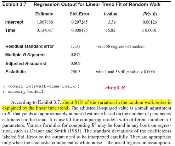
26 Consider the deterministic trend model Y t = µ t + X t. Let ˆµ t denote the estimated trend. We estimate X t by Y t ˆµ t, and the standard deviation γ0 of X t by the residual standard deviation s = 1 n (Y t ˆµ t ) n p 2 (6) where p is the number of parameters estimated in µ t and n p is the degree of freedom for s. The value of s (depent on the unit) gives an absolute measure of the goodness of fit of the estimated trend. A unitless measure of the goodness of fit is the R 2. (the coefficient of determination, or multiple R-squared). t=1 R 2 is the square of the sample correlation coefficient between the observed series and the estimated trend. R 2 is also the fraction of the variation in the series that is explained by the estimated trend.

27

28 3.6 Residual Analysis In the model Y t = µ t + X t, the unobserved stochastic component {X t } can be predicted by the residual ˆX t = Y t ˆµ t. We may investigate the standardized residual ˆX t /s. (most statistics software will produce standardized residuals using a more complicated standard error in the denominator that takes into account the specific regression model being fit.)

29 The expression rstudent(model3) returns the (externally) studentized residuals from the fitted model. [whereas rstandard(model3) gives the (internally) standardized residuals.] Exhibit 3.8 Residuals versus Time for Temperature Seasonal Means (chap3.r)

30 There are no apparent patterns relating to different months of the year. Exhibit 3.9 Residuals versus Time with Seasonal Plotting Symbols (chap3.r)

31 We look at the standardized residuals versus the corresponding trend estimate (fitted value). No dramatic patterns are found. Exhibit 3.10 Standardized Residuals versus Fitted Values for the Temperature Seasonal Means Model (chap3.r)

32 The normality of the standardized residuals may be checked by histogram and QQ plot. Gross nonnormality can be assessed by plotting a histogram of the residuals or standardized residuals.

33 Normality can be checked more carefully by plotting the so-called normal scores or quantile-quantile (QQ) plot. Such a plot displays the quantiles of the data versus the theoretical quantiles of a normal distribution. The straight-line pattern here supports the assumption of a normally distributed stochastic component in this model. qqnorm(rstudent(model3)) A reference straight line can be superimposed on the Q-Q normal score plot by qqline(rstudent(model3))

34

35 An excellent test of normality is known as the Shapiro-Wilk test. It essentially calculates the correlation between the residuals and the corresponding normal quantiles. shapiro.test(rstudent(model3)) The runs test tests the independence of a sequence of random variables by checking whether there are too many or too few runs above (or below) the median. runs(rstudent(model3))

36 The Sample Autocorrelation Function Another very important diagnostic tool for examining dependence is the sample autocorrelation function. Def. If {Y t } is a sequence of data, we define the sample autocorrelation function r k at lag k as r k = n t=k+1 (Y t Y )(Y t k Y ) n t=1 (Y t Y ) 2, for k = 1, 2, (7) A plot of r k versus lag k is often called a correlogram. When {Y t } is a stationary process, r k gives an estimate of ρ k.

37 win.graph(width=4.875, height=3, pointsize=8) acf(rstudent(model3)) Exhibit 3.13 Sample Autocorrelation of Residuals of Seasonal Means Model (chap3.r)

38 We now consider the standardized residuals from fitting a straight line to the rwalk dataset. Exhibit 3.14 Residuals from Straight Line Fit of the Random Walk (chap3.r)

39 Exhibit 3.15 Residuals versus Fitted Values from Straight Line Fit (chap3.r)

40 Exhibit 3.16 Sample Autocorrelation of Residuals from Straight Line Model (chap3.r)

41 Let us turn to the annual rainfall in Los Angeles (Exhibit 1.1). We found no evidence of dependence in that series, but we now look for evidence against normality. Exhibit 3.17 displays the normal quantile-quantile plot for that series. We see considerable curvature in the plot. Exhibit 3.17 Quantile-Quantile Plot of Los Angeles Annual Rainfall Series (chap3.r)

42 Exercises 3.6 & 3.12: The data file beersales contains monthly U.S. beer sales (in millions of barrels) for the period January 1975 through December (a) Display and interpret the time series plot for these data. (b) Now construct a time series plot that uses separate plotting symbols for the various months. Does your interpretation change from that in part (a)? (c) Use least squares to fit a seasonal-means trend to this time series. Interpret the regression output. Save the standardized residuals from the fit for further analysis. (d) Construct and interpret the time series plot of the standardized residuals from part (c). Be sure to use proper plotting symbols to check on seasonality in the standardized residuals. (e) Use least squares to fit a seasonal-means plus quadratic time trend to the beer sales time series. Interpret the regression output. Save the standardized residuals from the fit for further analysis. See TS-ch3.R

43 (f) Construct and interpret the time series plot of the standardized residuals from part (e). Again use proper plotting symbols to check for any remaining seasonality in the residuals. (g) Perform a runs test on the standardized residuals from part (e) and interpret the results. (h) Calculate and interpret the sample autocorrelations for the standardized residuals. (i) Investigate the normality of the standardized residuals (error terms). Consider histograms and normal probability plots. Interpret the plots. See TS-ch3.R