Advanced Machine Learning

Transcription

1 Advanced Machine Learning Lecture 4: Deep Learning Essentials Pierre Geurts, Gilles Louppe, Louis Wehenkel 1 / 52

2 Outline Goal: explain and motivate the basic constructs of neural networks. From linear discriminant analysis to logistic regresion Stochastic gradient descent From logistic regression to the multi-layer perceptron Vanishing gradients and recti ed networks Universal approximation theorem 2 / 52

3 Deep Learning / 52

4 Threshold Logic Unit The Threshold Logic Unit (McCulloch and Pitts, 1943) was the rst mathematical model for a neuron. Assuming Boolean inputs and outputs, it is de ned as: This unit can implement: or(a, b) = 1 {a+b 0.5 0} and(a, b) = 1 {a+b 1.5 0} not(a) = 1 { a+0.5 0} f(x) = 1 { w x +b 0} i i i Therefore, any Boolean function can be built witch such units. 4 / 52

5 Perceptron The perceptron (Rosenblatt, 1957) is very similar, except that the inputs are real: f(x) = { 1 0 if w x i i i + b 0 otherwise This model was originally motivated by biology, with x and and ring rates. i f This is a cartoonesque biological model. w i being synaptic weights 5 / 52

6 Let us de ne the activation function: σ(x) = { 1 0 if x 0 otherwise Therefore, the perceptron classi cation rule can be rewritten as T f(x) = σ(w x + b). 6 / 52

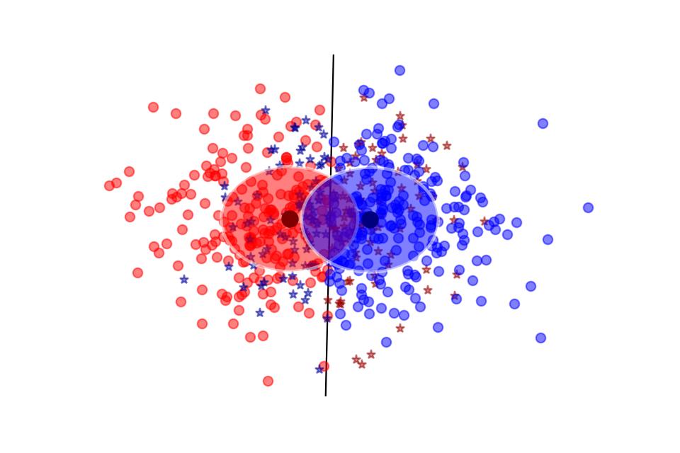
7 Linear discriminant analysis Consider training data x R p y {0, 1},. (x, y) P X,Y, with Assume class populations are Gaussian, with same covariance matrix (homoscedasticity): 1 1 P (x y) = exp ( (x μ ) Σ (x μ ) (2π) p Σ 2 Σ y T 1 y ) 7 / 52

8 Using the Bayes' rule, we have: P (x Y = 1)P (Y = 1) P (Y = 1 x) = P (x) P (x Y = 1)P (Y = 1) = P (x Y = 0)P (Y = 0) + P (x Y = 1)P (Y = 1) 1 =. P (x Y =0)P (Y =0) 1 + P (x Y =1)P (Y =1) 8 / 52

9 Using the Bayes' rule, we have: P (x Y = 1)P (Y = 1) P (Y = 1 x) = P (x) P (x Y = 1)P (Y = 1) = P (x Y = 0)P (Y = 0) + P (x Y = 1)P (Y = 1) 1 =. P (x Y =0)P (Y =0) 1 + P (x Y =1)P (Y =1) It follows that with 1 σ(x) =, 1 + exp( x) we get ( log P (x Y = 1) P (Y = 1) + log ) P (x Y = 0) P (Y = 0) P (Y = 1 x) = σ. 9 / 52

10 Therefore, P (Y = 1 x) = σ P (x Y = 1) log + log P (x Y = 0) P (Y = 1) P (Y = 0) a = σ ( log P (x Y = 1) log P (x Y = 0) + a) 1 = σ ( (x μ ) Σ (x μ ) + (x μ ) Σ (x μ 1 T ) + a 2 2 = σ (μ μ 1 0) T Σ x + w T = σ ( w T x + b) b 0 T 1 0 ) 1 T 1 (μ Σ μ μ Σ μ T 1 1) + a 2 10 / 52

11 11 / 52

12 11 / 52

13 11 / 52

14 Note that the sigmoid function σ(x) = exp( x) looks like a soft heavyside: Therefore, the overall model perceptron. T f(x; w, b) = σ(w x + b) is very similar to the 12 / 52

15 In terms of tensor operations, the computational graph of f can be represented as: where white nodes correspond to inputs and outputs; red nodes correspond to model parameters; blue nodes correspond to intermediate operations, which themselves produce intermediate output values (not represented). This unit is the core component all neural networks! 13 / 52

16 Logistic regression Same model as for linear discriminant analysis. But, ignore model assumptions (Gaussian class populations, homoscedasticity); instead, nd w, b P (Y = 1 x) = σ ( w T x + b) that maximizes the likelihood of the data. 14 / 52

17 We have, arg max P (d w, b) w,b = arg max P (Y = y x, w, b) w,b i i x i,y i d = arg max σ(w x + b) (1 σ(w x + b)) = arg w,b min w,b x i,y i d T y i T 1 y i i i T i i T i x i,y i d y log σ(w x + b) (1 y ) log(1 σ(w x + b)) L(w,b)= i l(y i, y^ (x i;w,b)) i This loss is an instance of the cross-entropy p = Y x i q = Y^ x for and. i H(p, q) = E [ log q] p 15 / 52

18 Y { 1, 1} When takes values in, a similar derivation yields the logistic loss L(w, b) = log σ y T ( i (w x i + b)) ). x i,y i d In general, the cross-entropy and the logistic losses do not admit a minimizer that can be expressed analytically in closed form. However, a minimizer can be found numerically, using a general minimization technique such as gradient descent. 16 / 52

19 Gradient descent L(θ) θ w b Let denote a loss function de ned over model parameters (e.g., and ). L(θ) To minimize, gradient descent uses local linear information to iteratively move towards a (local) minimum. θ R For, a rst-order approximation around can be de ned as 0 d L^ 0 0 T (θ + ϵ) = L(θ ) + ϵ θl(θ 0) + ϵ. 2γ θ / 52

20 A minimizer of the approximation is given for which results in the best improvement for the step. Therefore, model parameters can be updated iteratively using the update rule: Notes: θ 0 γ are the initial parameters of the model; is the learning rate; L^ (θ 0 + ϵ) ϵl^ (θ 0 + ϵ) = 0 1 = L(θ ) + θ 0 ϵ, γ θ = θ γ L(θ ) t+1 t θ t both are critical for the convergence of the update rule. ϵ = γ L(θ ) θ 0 18 / 52

21 Example 1: Convergence to a local minima 19 / 52

22 Example 1: Convergence to a local minima 19 / 52

23 Example 1: Convergence to a local minima 19 / 52

24 Example 1: Convergence to a local minima 19 / 52

25 Example 1: Convergence to a local minima 19 / 52

26 Example 1: Convergence to a local minima 19 / 52

27 Example 1: Convergence to a local minima 19 / 52

28 Example 1: Convergence to a local minima 19 / 52

29 Example 2: Convergence to the global minima 20 / 52

30 Example 2: Convergence to the global minima 20 / 52

31 Example 2: Convergence to the global minima 20 / 52

32 Example 2: Convergence to the global minima 20 / 52

33 Example 2: Convergence to the global minima 20 / 52

34 Example 2: Convergence to the global minima 20 / 52

35 Example 2: Convergence to the global minima 20 / 52

36 Example 2: Convergence to the global minima 20 / 52

37 Example 3: Divergence due to a too large learning rate 21 / 52

38 Example 3: Divergence due to a too large learning rate 21 / 52

39 Example 3: Divergence due to a too large learning rate 21 / 52

40 Example 3: Divergence due to a too large learning rate 21 / 52

41 Example 3: Divergence due to a too large learning rate 21 / 52

42 Example 3: Divergence due to a too large learning rate 21 / 52

43 Stochastic gradient descent In the empirical risk minimization setup, L(θ) L(θ) L(θ) 1 = l(y i, f(x i ; θ)) N x i,y i d and its gradient decomposes as 1 = l(y i, f(x i ; θ)). N x i,y i d Therefore, in batch gradient descent the complexity of an update grows linearly with the size of the dataset. N More importantly, since the empirical risk is already an approximation of the expected risk, it should not be necessary to carry out the minimization with great accuracy. 22 / 52

44 Instead, stochastic gradient descent uses as update rule: θ = θ γ l(y, f(x ; θ )) t+1 t i(t+1) i(t+1) t Iteration complexity is independent of. {θ t = 1,...} The stochastic process t depends on the examples picked randomly at each iteration. N i(t) 23 / 52

45 Instead, stochastic gradient descent uses as update rule: θ = θ γ l(y, f(x ; θ )) t+1 t i(t+1) i(t+1) t Iteration complexity is independent of. {θ t = 1,...} The stochastic process t depends on the examples picked randomly at each iteration. N i(t) Batch gradient descent Stochastic gradient descent 24 / 52

46 Why is stochastic gradient descent still a good idea? Informally, averaging the update over all choices θ = θ γ l(y, f(x ; θ )) t+1 t i(t+1) i(t+1) t i(t + 1) restores batch gradient descent. Formally, if the gradient estimate is unbiased, e.g., if 1 E [ l(y, f(x ; θ i(t+1) i(t+1) i(t+1) t ))] = l(y i, f(x i ; θ t )) N x i,y i d = L(θ ) t then the formal convergence of SGD can be proved, under appropriate assumptions (see references). When decomposing the excess error in terms of approximation, estimation and optimization errors, stochastic algorithms yield the best generalization performance (in terms of expected risk) despite being the worst optimization algorithms (in terms of empirical risk) (Bottou, 2011). x, y P i i X,Y Interestingly, if training examples are received and used in an online fashion, then SGD directly minimizes the expected risk. 25 / 52

47 Layers So far we considered the logistic unit, where,, w R p b R and. h = σ ( w T x + b) h R x R p These units can be composed in parallel to form a layer with T h = σ(w x + b) h R q x R p W R p q b R q outputs: where,,, and where is upgraded to the element-wise sigmoid function. q σ( ) 26 / 52

48 Multi-layer perceptron Similarly, layers can be composed in series, such that: where denotes the model parameters. This model is the multi-layer perceptron, also known as the fully connected feedforward network. Optionally, the last activation values. h 0 h 1... h L f(x; θ) = x T = σ(w h + b ) T = σ(w h + b L L 1 L ) = h L θ {W, b,... k = 1,..., L} y^ R σ k k can be skipped to produce unbounded output 27 / 52

49 28 / 52

50 To minimize with stochastic gradient descent, we need the gradient. Therefore, we require the evaluation of the (total) derivatives l L(θ) l(θ ) dl dw k of the loss with respect to all model parameters,, for. These derivatives can be evaluated automatically from the computational graph of using automatic differentiation., dl db k W b k k k = 1,..., L θ t l 29 / 52

51 Automatic differentiation Consider a 1-dimensional output composition f g, such that y u = f(u) = g(x) = (g (x),..., g (x)). 1 m The chain rule of total derivatives states that dy dx = m k=1 y u k du k dx recursive case Since a neural network is a composition of differentiable functions, the total derivatives of the loss can be evaluated by applying the chain rule recursively over its computational graph. The implementation of this procedure is called (reverse) automatic differentiation (AD). 30 / 52

52 As a guiding example, let us consider a simpli ed 2-layer MLP and the following loss function: f(x; W, W ) 1 2 l(y, ; W, W ) y^ 1 2 x R p y R W = σ ( W σ W 2 T ( 1 T x)) for,, and. 1 = cross_ent(y, y^ ) + λ ( W W 2 2) p q R W R 2 q 31 / 52

53 As a guiding example, let us consider a simpli ed 2-layer MLP and the following loss function: f(x; W, W ) 1 2 l(y, ; W, W ) y^ 1 2 x R p y R W = σ ( W σ W 2 T ( 1 T x)) for,, and. 1 = cross_ent(y, y^ ) + λ ( W W 2 2) p q R W R 2 q 32 / 52

54 The total derivative l W dl dw 1 can be computed backward, by walking through all paths from to in the computational graph and accumulating the terms: 1 dl dw 1 du 8 dw 1 = l du 8 u dw + = l u 4 du 4 dw 1 33 / 52

55 This algorithm is known as reverse-mode automatic differentiation, also called backpropagation. An equivalent procedure can be de ned to evaluate the derivatives in forward mode, from inputs to outputs. Automatic differentiation generalizes to inputs and outputs. if N M otherwise, if, reverse-mode automatic differentiation is computationally more ef cient. M N, forward automatic differentiation is better. Since differentiation is a linear operator, AD can be implemented ef ciently in terms of matrix operations. N M 34 / 52

56 Vanishing gradients Training deep MLPs with many layers has for long (pre-2011) been very dif cult due to the vanishing gradient problem. Small gradients slow down, and eventually block, stochastic gradient descent. This results in a limited capacity of learning. Backpropagated gradients normalized histograms (Glorot and Bengio, 2010). Gradients for layers far from the output vanish to zero. 35 / 52

57 Consider a simpli ed 3-layer MLP, with Under the hood, this would be evaluated as x, w, w, w R 1 2 3, such that f(x; w, w, w ) = σ w σ w σ w ( 3 ( 2 ( 1 x ))). u 1 u 2 u 3 u 4 u 5 y^ = w x 1 = σ(u ) 1 = w u 2 2 = σ(u ) 3 = w u 3 4 = σ(u ) 5 and its derivative d y^ dw 1 as d y^ = dw 1 y^ u 5 u 5 u 4 σ(u ) u 4 u 3 u 3 u 2 σ(u ) u 2 u 1 u 1 w 1 σ(u ) = w w 3 2 x u u u / 52

58 The derivative of the sigmoid activation function σ is: dσ dx 0 (x) dσ dx Notice that for all. 1 4 (x) = σ(x)(1 σ(x)) x 37 / 52

59 Assume that weights are initialized randomly from a Gaussian with zero-mean and small variance, such that with high probability. Then, w, w, w w 1 i d y^ dw 1 = σ(u 5) σ(u 3) σ(u 1) w w 3 2 u u u x This implies that the gradient layers in the network increases. d y^ dw 1 exponentially shrinks to zero as the number of Hence the vanishing gradient problem. In general, bounded activation functions (sigmoid, tanh, etc) are prone to the vanishing gradient problem. Note the importance of a proper initialization scheme. 38 / 52

60 Recti ed linear units Instead of the sigmoid activation function, modern neural networks are for most based on recti ed linear units (ReLU) (Glorot et al, 2011): ReLU(x) = max(0, x) 39 / 52

61 Note that the derivative of the ReLU function is d dx ReLU(x) = { 0 1 if x 0 otherwise For x = 0, the derivative is unde ned. In practice, it is set to zero. 40 / 52

62 Therefore, d y^ dw 1 σ(u 5) σ(u = w 3) σ(u w 1) 3 2 x u u u =1 =1 =1 This solves the vanishing gradient problem, even for deep networks! (provided proper initialization) Note that: The ReLU unit dies when its input is negative, which might block gradient descent. This is actually a useful property to induce sparsity. This issue can also be solved using leaky ReLUs, de ned as for a small (e.g., ). LeakyReLU(x) = max(αx, x) α R + α = / 52

63 Universal approximation Theorem. (Cybenko 1989; Hornik et al, 1991) Let be a bounded, non-constant continuous function. Let denote the -dimensional hypercube, and denote the space of continuous functions on. Given any and, there exists and such that satis es q > 0 σ( ) I p p C(I p) I p f C(I p) ϵ > 0 v, w, b, i = 1,..., q i i i F (x) = v σ(w x + b ) sup x I p i i T i i q f(x) F (x) < ϵ. It guarantees that even a single hidden-layer network can represent any classi cation problem in which the boundary is locally linear (smooth); It does not inform about good/bad architectures, nor how they relate to the optimization procedure. The universal approximation theorem generalizes to any non-polynomial (possibly unbounded) activation function, including the ReLU (Leshno, 1993). 42 / 52

64 Theorem (Barron, 1992) The mean integrated square error between the estimated network and the target function is bounded by F^ where is the number of training points, is the number of neurons, is the input dimension, and measures the global smoothness of. Combines approximation and estimation errors. f C qp ( + q N ) O log N f 2 N q p C f f Provided enough data, it guarantees that adding more neurons will result in a better approximation. 43 / 52

65 Consider the 1-layer MLP f(x) = w i ReLU(x + b i ). This model can approximate any smooth 1D function, provided enough hidden units. 44 / 52

66 Consider the 1-layer MLP f(x) = w i ReLU(x + b i ). This model can approximate any smooth 1D function, provided enough hidden units. 44 / 52

67 Consider the 1-layer MLP f(x) = w i ReLU(x + b i ). This model can approximate any smooth 1D function, provided enough hidden units. 44 / 52

68 Consider the 1-layer MLP f(x) = w i ReLU(x + b i ). This model can approximate any smooth 1D function, provided enough hidden units. 44 / 52

69 Consider the 1-layer MLP f(x) = w i ReLU(x + b i ). This model can approximate any smooth 1D function, provided enough hidden units. 44 / 52

70 Consider the 1-layer MLP f(x) = w i ReLU(x + b i ). This model can approximate any smooth 1D function, provided enough hidden units. 44 / 52

71 Consider the 1-layer MLP f(x) = w i ReLU(x + b i ). This model can approximate any smooth 1D function, provided enough hidden units. 44 / 52

72 Consider the 1-layer MLP f(x) = w i ReLU(x + b i ). This model can approximate any smooth 1D function, provided enough hidden units. 44 / 52

73 Consider the 1-layer MLP f(x) = w i ReLU(x + b i ). This model can approximate any smooth 1D function, provided enough hidden units. 44 / 52

74 Consider the 1-layer MLP f(x) = w i ReLU(x + b i ). This model can approximate any smooth 1D function, provided enough hidden units. 44 / 52

75 Consider the 1-layer MLP f(x) = w i ReLU(x + b i ). This model can approximate any smooth 1D function, provided enough hidden units. 44 / 52

76 Consider the 1-layer MLP f(x) = w i ReLU(x + b i ). This model can approximate any smooth 1D function, provided enough hidden units. 44 / 52

77 Consider the 1-layer MLP f(x) = w i ReLU(x + b i ). This model can approximate any smooth 1D function, provided enough hidden units. 44 / 52

78 (Bayesian) In nite networks Consider the 1-layer MLP with a hidden layer of size σ function : q and a bounded activation f(x) h (x) j ( j q j j j=1 p i=1 = b + v h (x) = σ a + u x i,j i) Assume Gaussian priors,, and a N (0, σ ) j a 2. v N (0, σ j v 2 ) b N (0, σ b 2 ) u N (0, σ ) i,j u 2 45 / 52

79 For a xed value, let us consider the prior distribution of implied by the prior distributions for the weights and biases. We have v h j (x ) x (1) f(x ) E[v h (x )] = E[v ]E[h (x )] = 0, j since and j are statistically independent and j has zero mean by hypothesis. The variance of the contribution of each hidden unit j (1) j j (1) (1) v h j is (1) V[v h (x )] j j (1) = E[(v h (x )) ] E[v h (x )] j j 2 j (1) 2 = E[v ]E[h (x ) ] j (1) 2 = σ E[h (x ) ], v 2 j (1) 2 j j (1) 2 which must be nite since (1) h j V (x ) = E[h (x ) ] is bounded by its activation function. We de ne, and is the same for all. j (1) 2 j 46 / 52

80 By the Central Limit Theorem, as q q v h (1) j=1 j j(x) f(x ) qσ V (x )., the total contribution of the hidden units,, to the value of becomes a Gaussian with variance v 2 (1) b σ (1) f(x ) σ + qσ V (x ) The bias is also Gaussian, of variance, so for large, the prior distribution is a Gaussian of variance. Accordingly, for, for some xed, the prior converges to a Gaussian of mean zero and variance as. For two or more xed values q σ = ω v vq 1 2 (1) (2) b 2 b 2 v 2 (1) x, x,... ω v f(x ) σ + ω σ b 2 v 2 v 2 V (x (1) ) q, a similar argument shows that, as, the joint distribution of the outputs converges to a multivariate Gaussian with means of zero and covariances of q (1) (1) (2) E[f(x )f(x )] q b 2 j=1 = σ + σ E[h (x )h (x )] v 2 j (1) j (2) (1) (2) = σ + ω b 2 2 (1) (2) vc(x, x ) C(x, x ) = E[h (x )h (x )] where and is the same for all. j (1) j (2) j 47 / 52

81 This result states that for any set of xed points of (1) (2) f(x ), f(x ),... is a multivariate Gaussian. (1) (2) x, x,..., the joint distribution In other words, the in nitely wide 1-layer MLP converges towards a Gaussian process. (Neal, 1995) 48 / 52

82 Effect of depth Theorem (Montúfar et al, 2014) A recti er neural network with input units and q (L 1)p p hidden layers of width q p can compute functions that have Ω(( ) q ) p linear regions. That is, the number of linear regions of deep models grows exponentially in q and polynomially in. L q Even for small values of and, deep recti er models are able to produce substantially more linear regions than shallow recti er models. p L L 49 / 52

83 Cooking recipe Get data (loads of them). Get good hardware. De ne the neural network architecture as a composition of differentiable functions. Stick to non-saturating activation function to avoid vanishing gradients. Prefer deep over shallow architectures. Optimize with (variants of) stochastic gradient descent. Evaluate gradients with automatic differentiation. 50 / 52

84 References Materials from the rst part of the lecture are inspired from the excellent Deep Learning Course by Francois Fleuret (EPFL, 2018). Lecture 3a: Linear classi ers, perceptron Lecture 3b: Multi-layer perceptron Further references: Introduction to ML and Stochastic optimization Why are deep neural networks hard to train? Automatic differentiation in machine learning: a survey 51 / 52

85 Quiz Explain the model assumptions behind the sigmoid activation function. Why is stochastic gradient descent a good algorithm for learning? (despite being a poor optimization procedure in general) What is automatic differentiation? Why is training deep network with saturating activation functions dif cult? Study the importance of weight initialization. What is the universal approximation theorem? 52 / 52