FORECASTING WITH REGRESSION

Transcription

1 FORECASTING WITH REGRESSION MODELS Overview of basic regression echniques. Daa analysis and forecasing using muliple regression analysis. 106 Visualizaion of Four Differen Daa Ses Daa Se A Daa Se B Daa Se C For each daa se: Mean of X = 9.0 Mean of Y = 7.5 Correlaion = 0.82 OLS Regression equaion: Y = X 0.5 Daa Se D All have very similar saisical properies, bu are visually quie differen!!! 107 1

2 Simple Linear Regression Model The populaion regression model: Dependen Variable y Populaion Y inercep i β Populaion Slope Coefficien 0 β 1 Independen Variable x i ε i Random Error erm Linear componen Random Error componen Simple Linear Regression Model Y Y i β 0 β 1 X i ε i Observed Value of Y for x i Prediced Value of Y for x i ε i Random Error for his X i value Slope = β 1 Inercep = β 0 x i X 2

3 Simple Linear Regression Equaion The simple linear regression equaion provides an esimae of he populaion regression line Esimaed (or prediced) y value for observaion i yˆ i Esimae of he regression inercep b 0 b Esimae of he regression slope 1 x i Value of x for observaion i The individual random error erms e i have a mean of zero e i - yˆ ) y ( yi i i -(b0 1 i b x ) The mahemaical form of he regression model The mos basic regression analysis mehod Ordinary Leas Squares (OLS) OLS is referred o in boh Excel and SPSS as "linear regression". The mahemaical form of he regression model is essenially an equaion y f ( x) When building a forecas model, we sar wih a specific equaion. This is called model specificaion. The relaionship could be linear and non linear. Various mahemaical forms could be aemped If he model properies do no work ou when calibraing, i can be respecified by replacing he variables on he righ hand side wih ohers ha seem o provide a more clear explanaion of he forecas variable

4 Ordinary Leas Squares (OLS) Coefficien Esimaors b 0 and b 1 are obained by finding he values of b 0 and b 1 ha minimize he sum of he squared residuals (errors), SSE: min SSE min min min n i1 e 2 i (y yˆ ) i i 2 i [y (b 0 b x )] Differenial calculus is used o obain he coefficien esimaors b 0 and b 1 ha minimize SSE 1 i 2 4

5 OLS Coefficien Esimaors b 1 The slope coefficien esimaor is n i1 (xi x)(yi y) n 2 (x x) i1 i Cov(x, y) s 2 x s r s And he consan or y inercep is b0 y b1x y x where sample correlaion coefficien s sxy r s s sample covariance Cov(x, y) xy x y (x x)(y y) i n 11 i The regression line always goes hrough he mean x, y Muliple Regression Analysis (MRA) a paricular mulivariae echnique MRA incorporaes informaion from several variables o predic he behavior of a given variable. If a researcher is ineresed in predicing he sales of a produc, MRA can be used o develop a model ha would poenially incorporae informaion from oher influenial variables. Once a regression model is developed i can be used o predic he sales ino he fuure if fuure projecions of hese oher influenial variables are available. (such as inernal facors of he firm, economic facors or demographic characerisics) 115 5

6 12.1 The Muliple Regression Model Idea: Examine he linear relaionship beween 1 dependen d (Y) & 2 or more independen d variables ibl (X i ) Muliple Regression Model wih K Independen Variables: Y inercep Populaion slopes Random Error Y β0 β1 X1 β2 X2 βk XK ε Muliple Regression Equaion The coefficiens of he muliple regression model are esimaed using sample daa Muliple regression equaion wih K independen variables: Esimaed (or prediced) value of y yˆ i b 0 Esimaed inercep b 1 x 1i Esimaed slope coefficiens b 2 x 2i b K x Ki 6

7 Regression (e.g., MRA) models developed using cross secional daa are used for predicing saic values or values ha do no have a ime elemen. This means ha values are no generaed for a specific dae and ha ime is irrelevan in predicing values. Wha deermines values for hese models are oher non ime dependen d facors e.g. house sales price=f(house's square fee of living space). 118 MRA models developed using ime series daa, on he oher hand, are used o predic values ha have a ime elemen. In oher words, values are deermined for specific daes since he model is buil by examining he relaionships amongs variables over ime. For example, in a housing sars model, an annual (or monhly) model will be developed by examining he correlaion beween he number of sars and oher facors such as ineres raes or household income for successive years (or monhs). If he model is used o predic fuure values, hen he prediced values are referred o as forecass

8 Three opions o forecas a variable of ineres, e.g. sales 1. Develop a forecas by examining he hisorical paern of sales and hen exend he paern forward o generae a forecas. In his approach, sales is o be forecased by using pas values of his variable. 2. Develop a forecas using a muliple regression model based on "saic" or cross secional informaion from oher variables highly correlaed wih sales. 3. Develop a forecas using a muliple regression model based on boh pas values (ime series) of he variable o be prediced and oher variables highly correlaed wih sales. The seps involved in building models for predicing saic or ime series values are almos idenical. 120 A muliple regression model based on "saic" or cross secional informaion This model would predic he level of sales given for example, he household income, unemploymen rae, and cusomer demographics. Noe ha up o dae cross secional daa on economic variables, such as household income, is difficul o obain. This daa can be compiled from Saisical Absracs as par of he populaion Census, bu his is only underaken every five years. Mos companies do no he have he resources or ime o conduc heir own demographic consumer surveys

9 A muliple regression model based on boh ime series of he variable and oher highly correlaed variables Generaesa a model using ime series daa (annual/quarerly/monhly) for boh sales and oher influencing facors. examine several variables generae a muliple regression model. This ype of daa may be more readily available since a single annual survey can be used o exrapolae informaion for many regions. Daa collecing agencies such as TUİK (Turkish Saisical Insiue), BIST (Borsa Isanbul) generally produce ime series daa 122 Model Building Mehodology The Sages of Saisical Model Building Model lspecificaion i * Coefficien Esimaion Model Verificaion Undersand he problem o be sudied Selec dependen and independen variables Idenify model form (linear, quadraic ) Deermine required daa for he sudy Inerpreaion and Inference 9

10 The Sages of Model Building Model Specificaion Coefficien Esimaion Model lverificaion Inerpreaion and Inference * (coninued) Esimae he regression coefficiens using he available daa Form confidence inervals for he regression coefficiens For predicion, goal is he smalles s e If esimaing individual slope coefficiens, examine model for mulicollineariy and specificaion bias The Sages of Model Building Model Specificaion Coefficien Esimaion Model lverificaion Inerpreaion and Inference * (coninued) Logically evaluae regression resuls in ligh of he model (i.e., are coefficien signs correc?) Are any coefficiens biased or illogical? Evaluae regression assumpions (i.e., are residuals random and independen?) If any problems are suspeced, reurn o model specificaion and adjus he model 10

11 The Sages of Model Building Model Specificaion (coninued) Coefficien Esimaion Model lverificaion Inerpreaion and Inference Inerpre he regression resuls in he seing and unis of your sudy Form confidence inervals or es hypoheses abou regression coefficiens Use he model for forecasing or predicion * A process for regression forecasing preliminary daa screening by graphics Look for rend, seasonal, and cyclical componens, as well as for ouliers. Deermine wha ype of regression model may be mos appropriae (e.g. Linear versus Nonlinear, or Trend versus Causal) generaion of a forecas model by MRA

12 Forecas model evaluaion In sample evaluaion (Rerospecive approach) When he model is evaluaed in comparison wih he daa used in specifying he model, we are deermining how well he model fis he daa. Ou of sample evaluaion When he model is evaluaed by using a holdou period, we can deermine how accurae he model is for an acualforecas horizon. Afer an evaluaion of fi and accuracy, he bes model should be respecified using he enire daa se. 128 Forecasing wih a Simple Linear Trend Example: For DPI daa (given from Jan 1993 hrough Dec 2005), develop a forecas for he las seven monhs of The linear ime rend model for DPI is DPI ˆ b 0 b where T, ime index, is usually se equal o 1 for he firs observaion T 12

13 Sequence char Pronounced rend! A linear rend line would fi he daa well. 130 Run Linear Regression o provide model coefficien esimaes PI ˆ 4542,54 28,91T D

14 Inerpreaion of he coefficien esimaes DPI ˆ 4542,54 28,91T The slope erm ells ha: On average, disposable personal income increased by 28,91 billion dollars per monh 132 Saisical Evaluaion of he regression model Saisical evaluaion suggess ha his linear equaion provides a very good fi o he daa

15 Using he equaion o make a forecas DPI ˆ 4542,54 28,91T forhe las seven monhs of 2005, subsiue he ime index values (T) from 150 o 156. Trend esimaes: June 2005: DPI = 4542,54+28, (150) = 8879,04 July 2005: DPI = 4542,54+28,91 (151) = 8907,95... Dec 2005: DPI = 4542,54+28,91 (156) = 9052, Noe We do no imply any sense of causaliy in such a model. dltime does no cause income orise. Income has increased over ime a a reasonably seady rae for reasons no explained by our model

16 Using a causal regression model o forecas y f ( x) Ina causal model, dl a change in he independen d variable ibl (X) is assumed o cause a change in he dependen variable (Y). Suppose ha a bivariae (simple) regression model will be developed for explaining and predicing he level of jewelery sales. Wha facors do you hink migh have an impac on jewelery sales? Some poenial causal variables: income, ineres raes, he unemploymen rae, so on. A subsanial seasonal aspec o jewelery sales can be expeced. 136 DPI JS? Consider how well jewelery sales (JS) can be forecas on he basisof disposablepersonal l income (DPI), as a measure of overall purchasing power. Develop a forecas of JS for each of he monhs of

17 Before developing a regression forecas model Look a ime paerns of he variables 138 Seasonal decomposiion of JS Deseasonalized JS daa shows he upward rend clearly

18 Look firs a scaer plo of JS and DPI Higher values of JS are associaed wih higher incomes The effec of seasonaliy is seen in a dramaic way. 140 Scaer Plo of seasonally adjused JS and DPI A linear line hrough h hose poins could provide a reasonably good fi o he daa. See also all of hese observaions are well away from he origin!

19 Regression Resuls for Original JS Daa J Sˆ b0 b1 DPI J Sˆ 88,738 0,265 DPI 142 Using he equaion o make a forecas J Sˆ 88,738 0,265 DPI To use his model dlo forecas JS for each monh of 2005, DPI forecass for he same period should be obained. Hol s Exponenial Smoohing forecas for DPI

20 Hol s Exponenial Smoohing forecas for DPI 144 Forecas JS for each monh of 2005 dae DPI esimae JS forecas JAN ,5 2518,66 FEB ,1 2526,23 Mar ,8 2533,84 APR ,5 2541,45 May ,2 2549,05 JUN ,9 2556,66 JUL ,6 2564,26 AUG ,3 2571,87 SEP ,0 2579,47 OCT ,7 2587,08 NOV ,4 2594,68 DEC ,1 2602,29 Upward rend in JS is accouned for by he regression model bu he seasonaliy is no aken ino accoun!! Thus, 2005 forecass are likely o be subsanially incorrec

21 ? How o incorporae seasonaliy in regression modeling 1. Eiher use a model ha can accoun for seasonaliy direcly 2. Or, deseasonalize he daa before developing he regression forecasing model * Developing a model based on seasonally adjused jewelery sales daa (SAJS) and reinroduce he seasonaliy as forecass being developed 146 Regression Model for SAJS Daa S AJS ˆ b0 b1 DPI SAJS ˆ 381,44 0,219DPI

22 SAJS as a funcion of DPI SAJS ˆ 381,44 0,219DPI dae Acual SAJSAJS forecas Error squared JAN , , ,12 FEB , , ,25 Mar , ,11 862,70 APR , ,39 223,42 May , , ,65 JUN , , ,29 JUL , , ,86 AUG , , ,79 SEP , , ,03 OCT , , ,03 NOV , , ,77 DEC , ,68 607,49 MSE= ,40 RMSE= 492, JS Final Forecas for 2005 i. Trend for SAJS is forecased ii. These are muliplied by he seasonal indices o ge he final forecas. reseasonalized dae Acual JS SAJS forecas seasonal indices JS forecas Error squared JAN , ,47 FEB , ,39 Mar , ,14 APR , ,71 May , ,40 JUN , ,65 JUL , ,85 AUG , ,71 SEP , ,91 OCT , ,45 NOV , ,67 DEC , ,34 MSE= ,69 RMSE= 466,

23 Linear Regression Assumpions For a given value of X, he populaion of Y values is normally disribued abou he populaion regression line. The rue relaionship form is linear (Y is a linear funcion of X, plus random error) The error erms are random variables wih mean 0 and consan variance, σ 2 The dispersion of populaion daa poins around he populaion regression line remains consan everywhere along he line. The uniform variance propery is called homoscedasiciy. A violaion of his assumpion is called heeroscedasiciy. The error erms, ε i are independen of each oher. This assumpion implies a random sample of X Y daa poins. When he X Y daa poins are recorded over ime, his assumpion is ofen violaed. Raher han being independen, consecuive observaions are serially correlaed (serial correlaion problem)

24 Basic Diagnosic Checks for Model Evaluaion 1. Ask yourself wheher he sign on he slope erm makes sense. i.e., are coefficien signs correc? Wha if he signs do no make sense? DPI ˆ 4542,54 28,91T J Sˆ 88,738 0,265 DPI SAJS ˆ 381,44 0,219DPI 152 Basic Diagnosic Checks for Model Evaluaion 2. Wheher or no he slope erm is significanly posiive or negaive?

25 Inference abou he Slope: Tes es for a populaion slope Is here a linear relaionship beween X and Y? Null and alernaive hypoheses H 0 : β 1 = 0 (no linear relaionship) H 1 : β 1 0 (linear relaionship does exis) Tes saisic b1 β s b 1 1 where: b 1 = regression slope coefficien β 1 = hypohesized slope s b1 = sandard error of he slope Hypohesis Tes for Populaion Slope Using he F Disribuion F Tes saisic shows he overall qualiy of he model F MSR MSE where MSR SSR k SSE MSE n k 1 where F follows an F disribuion wih k numeraor and (n k 1) denominaor degrees of freedom (k = he number of independen variables in he regression model) 25

26 Hypohesis Tes for Populaion Slope Using he F Disribuion (coninued) An alernae es for he hypohesis ha he slope is zero: H 0 : β 1 = 0 H 1 : β 1 0 Use he F saisic F MSR MSE SSR 2 s e The decision rule is rejec H 0 if F F 1,n 2,α As a general rule of humb, an F Saisic greaer han 4 is accepable and represens a well fied model. However, significanly larger F value readings are preferable. Regression Model for SAJS Daa SAJS ˆ 381,44 0,219DPI P value for he F Tes H 0 : β 1 = 0 H 1 : β 1 0 ( = 0,05) F raio=832,755 (p value=0,000 < α=0,05). There is sufficien evidence ha DPI affecs Seasonally Adjused Jewelery Sales (SAJS) Since P value < α, he esimaed coefficiens, b 0 and b 1, are saisically significan

27 Basic Diagnosic Checks for Model Evaluaion 3. Evaluae wha percen of he variaion (i.e. Up and down d movemen) in he dependen d variable is explained by variaion in he independen variable? R squared: he coefficien of deerminaion 2 2 R r 158 Explanaory Power of a Linear Regression Equaion Toal variaion is made up of wo pars: SST SSR SSE Toal Sum of Squares Regression Sum of Squares Error (residual) Sum of Squares 2 SST (y SSR (y ˆ y) SSE (y y ˆ 2 i y ) where: y i ) = Average value of he dependen variable y i = Observed values of he dependen variable ŷ i = Prediced value of y for he given x i value 2 i i) 27

28 Analysis of Variance (ANOVA) SST = oal sum of squares Measures he variaion of he y i values around heir mean, y SSR = regression sum of squares Explained variaion aribuable o he linear relaionship beween x and y SSE = error sum of squares Variaion aribuable o facors oher han he linear relaionship beween x and y Analysis of Variance (ANOVA) (coninued) 28

29 Coefficien of Deerminaion, R 2 The coefficien of deerminaion is he porion of he oal variaion in he dependen variable ha is explained by variaion in he independen variable The coefficien of deerminaion is also called R squared and is denoed as R 2 R 2 SSR SST regression sum of squares oal sum of squares noe: 0 R 2 1 Examples of Approximae r 2 Values Y r 2 = 1 Y r 2 = 1 X Perfec linear relaionship beween X and Y: 100% of he variaion in Y is explained by variaion in X r 2 = 1 X 29

30 Examples of Approximae r 2 Values Y 0 < r 2 < 1 Y X Weaker linear relaionships beween X and Y: Some bu no all of he variaion in Y is explained by variaion in X X Examples of Approximae r 2 Values Y r 2 = 0 r 2 = 0 X No linear relaionship beween X and Y: The value of Y does no depend on X. (None of he variaion in Y is explained by variaion in X) 30

31 Regression Model for SAJS Daa SAJS ˆ 381,44 0,219DPI 85,4% of he variaion in SAJS is explained by variaion in DPI 166 * Using he sandard error of he esimae s e is a measure of he variaion of observed y values from he regression line Y Y small s s e X large s e X The magniude of s e should always be judged relaive o he size of he y values in he sample daa 31

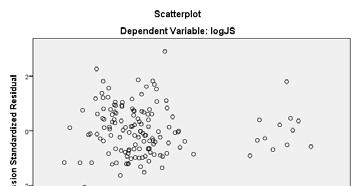
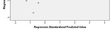
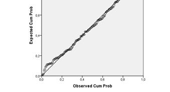
32 Regression Model for SAJS Daa SAJS ˆ 381,44 0,219DPI s e = $109 ($Millions) is moderaely small relaive o SAJS in he $1099 $2572 ($Millions) range 168 Analysis of Residuals Errors (residuals) from he regression model: e i = (y i y i ) < Assumpions: The underlying relaion is linear. The model errors are independen The errors have a consan variance The errors are normally disribued These residual plos are used in muliple regression: Residuals vs. Fied values of y Hisogram of he residuals PP plo for normaliy Residuals vs. ime (if ime series daa) Use he residual plos o check for violaions of regression assumpions

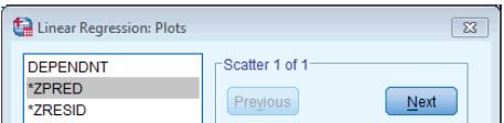
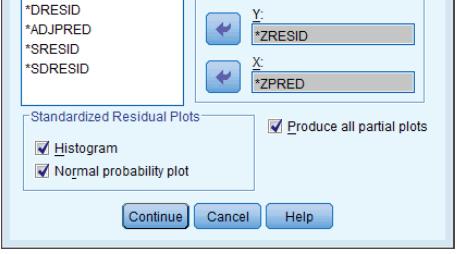
33 Regression plos in SPSS

34 * Serial correlaion also called auocorrelaion Auocorrelaion in he residuals is caused by a couple of reasons: Omission of criical variables from he model: since many economic variables end o exhibi an auocorrelaed paern, if an auocorrelaed explanaory variable has been excluded from he regression model, is influence will be echoed in he residuals. Using he incorrec mahemaical form of he model: if he mahemaical form of he model used is significanly differen from he rue form of he relaionship, li he residual may show he serial correlaion. For example, if a linear model is used insead of a muliplicaive model, he residual may be serially correlaed. 172 Auocorrelaed Errors Independence of Errors Error values are saisically independen Auocorrelaed Errors Residuals in one ime period arerelaed o Residuals in one ime period are relaed o residuals in anoher period 34

35 Auocorrelaed Errors Auocorrelaion violaes a leas squares regression assumpion Leads o s b esimaes ha are oo small (i.e., biased) Thus values are oo large and some variables may appear significan when hey are no (coninued) Auocorrelaion Auocorrelaion is correlaion of he errors ( id l ) i (residuals) over ime Time () Residual Plo Here, residuals show a cyclic paern, no random Residuals Time () Violaes he regression assumpion ha residuals are random and independen 35

36 Residual Analysis for Independence No Independen Independen residuals X res siduals X residuals X The Durbin Wason Saisic The Durbin Wason saisic is used o es for auocorrelaion H 0 : successive residuals are no correlaed (i.e., Corr(ε,ε 1 ) = 0) H 1 : auocorrelaion is presen If auocorrelaion is deeced, he OLS mehod of esimaing he coefficiens canno be used. 36

37 The Durbin Wason Saisic H 0 : ρ = 0 (no auocorrelaion) H 1 : auocorrelaion i is presen The Durbin Wason es saisic (d): d n 2 (e 2 e 1) n 1 e 2 The possible range is 0 d 4 d should be close o 2 if H 0 is rue d less han 2 may signal posiive auocorrelaion, d greaer han 2 may signal negaive auocorrelaion Tesing for Posiive Auocorrelaion H 0 : posiive auocorrelaion does no exis H 1 : posiive auocorrelaion is presen Calculae he Durbin Wason es saisic = d d can be approximaed by d = 2(1 r), where r is he sample correlaion of successive errors Find he values d L and d U from he Durbin Wason able (for sample size n and number of independen variables K) Decision rule: rejec H 0 if d < d L Rejec H 0 Inconclusive Do no rejec H 0 0 d L d U 2 37

38 Negaive Auocorrelaion Negaive auocorrelaion exiss if successive errorsarenegaively correlaed This can occur if successive errors alernae in sign Decision rule for negaive auocorrelaion: rejec H 0 if d > 4 d L ρ 0 ρ 0 Do no rejec H 0 Rejec H 0 Inconclusive Inconclusive Rejec H 0 0 d L d U 2 4 d U 4 d L 4 Tesing for Posiive Auocorrelaion Example wih n = 25: (coninued) Durbin-Wason Calculaions Sum of Squared Difference of Residuals Sum of Squared Residuals Durbin-Wason Saisic Sales y = x R 2 = Time d n 2 (e e n 1 e 2 )

39 Tesing for Posiive Auocorrelaion Here, n = 25 and here is K = 1 independen variable Using he Durbin Wason able, d L = and d U = (coninued) D = < d L = 1.29, so rejec H 0 and conclude ha significan posiive auocorrelaion exiss Therefore he linear model is no he appropriae model o forecas sales Decision: rejec H 0 since D = < d L Rejec H 0 Inconclusive Do no rejec H 0 0 d d U = L =1.29 Esimaion of Regression Models wih Auocorrelaed Errors Suppose ha we wan o esimae he coefficiens of he regression model y β 0 β x 1 1 β 2 x 2 β K x K ε where he error erm ε is auocorrelaed Two seps: (i) Esimae he model by leas squares, obaining he Durbin Wason saisic, d, and hen esimae he auocorrelaion parameer using r 1 d 2 39

40 Esimaion of Regression Models wih Auocorrelaed Errors (coninued) (ii) Esimae by leas squares a second regression wih dependen variable (Y ry 1 ) independen variables (X 1 rx 1, 1 ), (X 2 rx 2, 1 ),..., (X K rx K, 1 ) The parameers 1, 2,..., k are esimaed regression coefficiens from he second model An esimae of 0 is obained by dividing he esimaed inercep for he second model by (1 r) Hypohesis ess and confidence inervals for he regression coefficiens can be carried ou using he oupu from he second model Heeroscedasiciy Homoscedasiciy The probabiliy disribuion of he errors has consan variance Heeroscedasiciy The error erms do no all have he same variance The size of he error variances may depend on he size of he dependen variable value, for example 40

41 Heeroscedasiciy (coninued) When heeroscedasiciy is presen: leas squares is no he mos efficien procedure o esimae regression coefficiens The usual procedures for deriving confidence inervals and ess of hypoheses is no valid Residual Analysis for Homoscedasiciy Y Y x x residuals Non consan variance x residuals Consan variance x 41

42 Tess for Heeroscedasiciy To es he null hypohesis ha he error erms, ε i, all have he same variance agains he alernaive i ha heir variances depend on he expeced values ŷ i Esimae he simple regression e 2 i a 0 a yˆ 1 i Le R 2 be he coefficien of deerminaion of his new regression The null hypohesis is rejeced if nr 2 is greaer han 2 1, where 2 1, is he criical value of he chi square random variable wih 1 degree of freedom and probabiliy of error Generaion of a forecas model by MRA 1. Invesigae all he facors (explanaory variables) ha will influence he dependen variable (e.g. sales) and caegorize he daa by ype. 2. Describe he appropriae mahemaical form of he regression model o use given he available daa ypes. 3. Examine he relaionship beween he explanaory variable and he dependen variables using correlaion marix. 4. Selec he variables for model calibraion and esimae he model. This sep also involves evaluaing he model properies. coninued

43 Generaion of a forecas model by MRA 5. Inerpre coefficiens for explanaory variables, confirming heir saisical significance and raionalizing heir relaive size and sign (posiive/negaive). 6. Tes and evaluae he model. 7. Use he model o generae a forecas, applying he regression equaion o daa beyond ha used o creae he model. 8. Sae conclusions abou he qualiy of he model (e.g., abiliy o predic reliable oucomes). 190 Sep 1: Invesigae all facors influencing he forecas variable MRA involves esimaing he value of one variable based on daa from oher variables. For he jewelery sales (JS) forecas, key influencing facors could be: Disposable personal income (DPI) expeced sign of coefficien is posiive (posiive relaion bw JS and DPI) The unemploymen rae (UR) expeced sign negaive (likely inverse relaion bw JS and DPI) Thus: Dependen variable: JS Independen variables: DPI (in consan 1996 dollars) UR The wo independen variables are boh demand side facors. All hree variables are ime series daa. In considering he se of independen variables o use, we should find ones ha are no highly correlaed wih one anoher (Because of mulicollineariy problem)

44 JewelrySales versus Disposable Personal Income and Unemploymen 3 dimenional scaer As UR increases, JS decrease (while DPI is held consan) As DPI increases (while UR is held consan), JS increases. 192 Pracice Noe: Forecasing Explanaory Variables In selecing explanaory variables for a forecas model, a crucial limiaion is ha a forecas of hese variables is required. For insance, if he developer selecs he disposablepersonal l income (DPI) and unemploymen rae (UR) as he explanaory variables for he jewelery sales regression model, hen he developer will need a forecas of hese variables in order o generae a forecas of jewelery sales (JS). The developer would have o eiher purchase a forecas of DPI and UR from a forecasing agency or develop heir own forecas. The regression model specifies he relaionship beween he independen variables and he dependen variable. Therefore, if he fuure values of he independen variables are available hen he relaionship can be used calculae he fuure values of he dependen variable. However, i is imporan ha he forecas of he independen variables be reliable. For his reason, i is good pracice o choose independen variables ha are regularly forecas by an independen saisical agency like TUİK

45 Sep 2: The mahemaical form of he regression model The mos basic regression analysis mehod Ordinary Leas Squares (OLS) OLS is referred o in boh Excel and SPSS as "linear regression". The mahemaical form of he regression model is essenially an equaion y f ( x) When building a forecas model, we sar wih a specific equaion. This is called model specificaion. The relaionship could be linear and non linear. Various mahemaical forms could be aemped If he model properies do no work ou when calibraing, i can be respecified by replacing he variables on he righ hand side wih ohers ha seem o provide a more clear explanaion of he forecas variable. 194 Model specificaion for Jewelery Sales MRA The relaionship iniially examined beween he explanaory variables (DPI, UR) and dependen variable (JS) for our forecas model is: JS β β1 DPI β2 UR 0 For his model, he esimaed equaion would be: J Sˆ b This is a linear model, because all he parameers appear as muliples of he variables or he consan, and are added ogeher. 0 b1 DPI b 2 UR ε

46 Linear Models J Sˆ JSˆ b b Srucural Examples J Sˆ b0 b1 DPI 0 b1 DPI 0 b 1 DPI b 2 b UR 2 DPI 2 Non Linear Models J Sˆ b * DPI J Sˆ 0 b * DPI 0 b 1 b * UR 1 b Modelling Limiaions The model is a simplified represenaion of a real world relaionship. li Jus as archiecs build simplified models of buildings, analyss build simplified models of he world. By necessiy, hese models mus leave ou some informaion, bu hopefully capure he imporan pars of he relaionship

47 Sep 3: Examine he relaionship beween he explanaory variable and he dependen variables Analyze Correlae Bivariae The bes model is one where he explanaory variables are highly correlaed wih he dependen variable, and where he explanaory variables are no relaed o each oher. 198 Sep 4: Selec he variables for model calibraion and esimae he model Model Calibraion To evaluae a regression model, here are hree key saisics o consider: 1. The Durbin Wason (DW) saisic 2. The F saisic 3. The Adjused R 2 Saisics Used in Evaluaing Regression Models

48 Adjused R 2 The adjused R squared is an adjused measure of he coefficien of deerminaion (R 2 ). Adding variables o a regression will almos always increase he R 2, because mos variables will have some correlaion wih he dependen variable, even if ha correlaion is very low. The adjused R 2 is useful in helping he analys achieve he wo objecives in designing a model: Explain as much of he dependen variable as possible. Make he model as simple as possible

49 Oupus for JS muliple regression model The adjused R Square is quie low. Because many of he daa poins are quie a disance above or below he esimaed regression plane. The regression equaion explains only 7.5% of he variaion in jewelery sales volume. For n=144, α=0,05, k=2 independen variables: d L = 1,63 d U =1,72 (from Durbin Wason able) d L = 1,63 d U =1,72 4 d U = 2,28 4 d L = 2,37 There is no serial correlaion in he regression residuals 202 The ANOVA able shows he F saisic is relaively large and significan (an F Value above 4 is generally considered significan)

50 Sep 5: Inerpreing Coefficiens The unsandardized coefficiens (B): These are he esimaed coefficien values ( ). The value shows he relaionship of he explanaory variable on he dependen variable. The coefficien represens he parial effec of he independen variable on he dependen variable, holding all oher effecs consan. For example, if he variable coefficien is 10, hen a one uni change in he explanaory variable (also called he "regressor") will increase he dependen variable by 10. The sandardized coefficiens (Bea): The Bea value indicaes he relaive imporance of he variable in he model. A high absolue value indicaes ha he variable is very imporan while a low value indicaes ha he variable conribues lile o he model's predicive capaciy. Sd. Error (sandard error): This is he sandard error of he coefficien. This is required o deermine wheher he esimaed coefficien is significanly differen from zero. We usually wan he sandard error of he esimae o be less han half he size of he coefficien. The sandard error is required o calculae he value. The value: The value is calculaed by dividing he coefficien by he sandard error. The saisic deermines if he esimaed coefficien is significanly differen from zero. A value above 2 is considered significan. However, he saisic here can be ignored, because he "Sig" column inerpres is saisical significance for us. Sig. (Significance): The "Sig." column provides he significance level of he coefficien. The lower he Sig. Value, he higher he significance of he variable in he model. Usually, we require a level of significance smaller han 0.05 (95% confidence level), wih his indicaing fair confidence ha he coefficien is no equal o zero. In oher words, we can be quie sure ha his variable has a leas some parial influence on he arge variable, holding oher variables consan. If a variable is found o no be significan by a wide margin, you should srongly consider removing i from he equaion. 204 Sandardized bea (Bea) values are measured in sandard deviaion unis and so are direcly comparable. The "Bea" value is highes for DPI (.275), showing his o be he mos imporan variable in he regression. DPI has more impac in he model, his predicor is making a significan conribuion o he model. UR is insignifican, p value = 0,484 < 0,05. Signs of he coefficiens are esimaed as expeced. As he adjused R Square is quie low, he regression model needs o be improved

51 206 Mulicollineariy Where explanaory variables are relaed o each oher, he model suffers from mulicollineariy. This causes low significance of coefficiens and a high F saisic for he regression, meaning resuls may be unreliable or misleading in predicing he dependen variable

52 Suggesed mehods for removing mulicollineariy for regression esimaion. Remove one of he srongly correlaed explanaory variables from he model building process. If possible, generae a single new variable ha incorporaes informaion from boh correlaed explanaory variables. The variable selecion process should be resriced o explanaory variable ha have zero or only modes amouns of collineariy. Generally, o avoid mulicollineariy, any correlaion over +/ 0.5 should be examined, alhough hese correlaions do no usually creae serious collineariy problems unil hey are over +/ he coefficien able includes wo more columns: Tolerance and VIF. The variable's olerance describes he proporion of variance explained by his one variable ha is no explained by any oher variable. If he olerance is low (less hen 0.3), hen he variable could be deleed from he model wih lile loss of informaion. The VIF is he "variance inflaion facor". I is large if he variable is collinear wih oher variables and small if he variables are independen from one anoher. Ideally, he VIFs will all be less han 3.3 (he olerance and VIF are direcly relaed, wih VIF = 1/Tolerance)

53 Collineariy Saisics for JS regression The collineariy saisics show no evidence of a mulicollineariy problem. VIF=~ 1 < Example of a mulicollineariy problem The above coefficiens able indicaes he presence of mulicollineariy as he VIF value for he T Bill rae and 5 year morgage rae is well above 3.3. The correlaion beween hese variables.is 0.957, hus he T Bill variable is removed and regression model is redeveloped

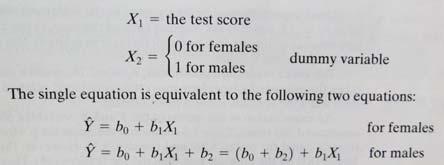
54 Dummy Variables Accouning for Seasonaliy in a MR model Can be used o measure a qualiaive aribue as seasons, gender, inervenions, i ec

55 Using Regression o forecas seasonal daa 55

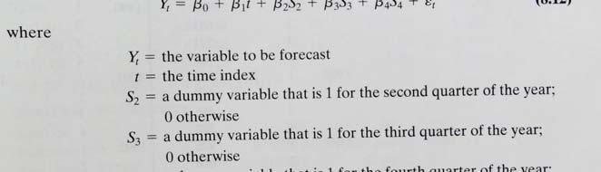
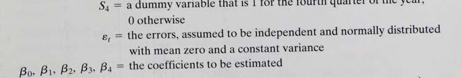
56 Time relaed explanaory variables Seasonal dummy variables Assumpion: he seasonal componen is unchanging from year o year D1=1 if hemonh h is January, 0 oherwise; D2=1 if he monh is February, 0 oherwise;.. D11=1 if he monh is November, 0 oherwise. Trading day variaion Assumpion: sales daa ofen vary according o he day of he week T1 = he number of imes Monday occurred in ha monh; T2 = he number of imes Tuesday occurred in ha monh;.. T7 = he number of imes Sunday occurred in ha monh. Time relaed explanaory variables Variable holiday effecs The effec of New Year on monhly sales daa Use seasonaldummy variable for December The effec of Ramadan Bairam I can occur in differen monhs every year V = 1 ifanyparof he Ramadan period falls in ha monh and zero oherwise. Inervenions Can occur when here is some ouside influence a a paricular ime which affecs he forecas variable. E.g. Inroducion of sea bels may have caused he number of road faaliies oundergo a levellshif downward. d To measure he effec of he sea bel inroducion Use a dummy variable consising of 0 s before he inroducion of sea bels and 1 s afer ha monh. 56

57 Time relaed explanaory variables Adverising expendiure he effec of adverising which lass for some ime beyond he acual adverising campaign. To include several weeks (or monhs) adverising expendiure: A1 = adverising expendiure for he previous monh; A2 = adverising expendiure for wo monhs previously;.. A1 = adverising expendiure for m monhs previously. Improvemens in JS regression model Remember JS ime series is quie seasonal wih some rend. Adding Dummy Variables Accouning for Seasonaliy Seasonal dummy variables for he 11 monhs of each year February hrough December. Effec of 9 Sepember A dummy variable for 911 effec ha equals 1 in Sepember and Ocober

58 Rerunning he regression model 220 Adjused R 2 has increased from 7,5 o 96,6 percen. Sandard Error of regression has fallen TheF saisics has increased Durbin Wason saisics indicaes ha no firs order serial correlaion is presen

59 Model coefficiens have he correc signs and are saisically significan, as indicaed by he high values and he corresponding low Sig. values. Consan erm and 911 effec are no significan and do no conribue o he model. The collineariy saisics show no evidence of a mulicollineariy problem

60 Pu simply, we wan a model where he residuals or errors (he difference beween he acual value of JS and he esimaed value) exhibi a paern ha mees specified crierion or properies. The errors are approximaely normally disribued The errors have no a consan variance!! Use ransformaion for improvemen. 224 Variable Transformaions Four mos common funcions The reciprocal The log (or Ln) The square roo The square

61

62 Sep 6: Use he Model o Generae a Forecas If he esimaed model is valid (boh saisically and hrough judgmen), we can use he resuls o generae a fuure forecas. We would only be comforable using he equaion o produce a forecas if we were fairly sure eiher ha: a. The independen variables acually cause he values of he prediced variable; or b. he relaionship ha shows correlaion beween he variable o be forecas and he variables in he equaion is likely o coninue. 228 Appendix: Correcing Heeroskedasiciy For auocorrelaion funcion: Choose Analyze Forecasing Auocorrelaions i Naural log ransform. For ARIMA: Choose Analyze Forecasing Creae Models. Under "Mehod", choose ARIMA; clickcrieria and selec Naural log ransform under "Transformaion"