10. Linear Models and Maximum Likelihood Estimation

Transcription

1 10. Linear Models and Maximum Likelihood Estimation ECE 830, Spring 2017 Rebecca Willett 1 / 34

2 Primary Goal General problem statement: We observe y i iid pθ, θ Θ and the goal is to determine the θ that produced {y i } n i=1. Given a collection of observations y 1,..., y n and a probability model p(y 1,..., y n θ) parameterized by the parameter θ, determine the value of θ that best matches the observations. 2 / 34

3 Estimation Using the Likelihood Definition: Likelihood function p(y θ) as a function of θ with y fixed is called the likelihood function. If the likelihood function carries the information about θ brought by the observations y = {y i } i, how do we use it to obtain an estimator? Definition: Maximum Likelihood Estimation θ MLE = arg max θ Θ p(y θ) is the value of θ that maximizes the density at y. Intuitively, we are choosing θ to maximize the probability of occurrence for y. 3 / 34

4 Maximum Likelihood Estimation MLEs are a very important type of estimator for the following reasons: MLE occurs naturally in composite hypothesis testing and signal detection (i.e., GLRT) The MLE is often simple and easy to compute MLEs are invariant under reparameterization MLEs often have asymptotic optimal properties (e.g. consistency (MSE 0 as N ) 4 / 34

5 Computing the MLE If the likelihood function is differentiable, then θ is found from log p(y θ) θ = 0 If multiple solutions exist, then the MLE is the solution that maximizes log p(y θ). That is, take the global maximizer. Note: It is possible to have multiple global maximizers that are all MLEs! 5 / 34

6 Example: Estimating the mean and variance of a Gaussian y i = A + ν i, ν i iid N (0, σ 2 ), i = 1,, n log p(y θ) A Note: σ 2 is biased! θ = [A, σ 2 ] = 1 n σ 2 (y i A) i=1 log p(y θ) σ 2 = n 2σ σ 4 Â = 1 n σ 2 = 1 n n i=1 y i n (y i A) 2 i=1 n (y i Â)2 i=1 6 / 34

7 Example: Stock Market (Dow-Jones Industrial Avg.) p({y i } i A, B) = 1 (2πσ 2 exp ) n/2 Based on this plot we might conjecture that the data is on average increasing. Probability model: y i = A + Bi + ν i A, B are unknown parameters, ν i white Gaussian noise to model fluctuations. { 1 2σ 2 } n (y i A Bi) 2 i=1 7 / 34

8 Example: A modern Example - Imaging Image processing can involve complicated estimation problems. For example, suppose we observe a moving object with noise. This image is blurry and noisy and our goal is to restore this image by debarring and denoising. 8 / 34

9 Example: A modern Example - Imaging We can model the moving part of the observed image as y = }{{} θ + }{{} ν noise-free blurry image noise = x}{{ w} +ν motion blur (convolution) where the parameter of interest w is the ideal (non-blurry) image and x represents the blur model or point spread function. Observation model: y =Xw + ν, ν N(0, σ 2 I) y N (Xw, σ 2 I) where X is a circulant matrix with the first row corresponding to x. 9 / 34

10 Linear Models and Subspaces The basic linear model is: θ = Xw where θ R n, X R n p with n > p is known and full rank, and w R p is a p-dimensional parameter or weight vector. In other words, we can write p θ = w i x i i=1 where w i is the i th element of w and x i is the i th column of X. We say that θ is in a subspace spanned by the columns of X 10 / 34

11 Subspaces Consider a set of vectors x 1, x 2,..., x p R n. The span of these vectors is the set of all vectors θ R n that can be generated from linear combinations of the set } p span ({x i } p i=1 {θ ) := : θ = w i x i, w 1,..., w p R i=1 p-dimensional subspace If the x 1,..., x p R n are linearly independent, then their span is a p-dimensional subspace of R n. Hence, even though the signal θ is a length-n vector, the fact that it lies in the subspace X means that it is actually a function of only p n free parameters or degrees of freedom. 11 / 34

12 Example: n = 3 x 1 = x 2 = X = span (x 1, x 2 ) = a b : a, b R Example: n = 3 x 1 = 1/ 2 1/ 2 0 X = span (x 1, x 2 ) = x 2 = a a b : a, b R 12 / 34

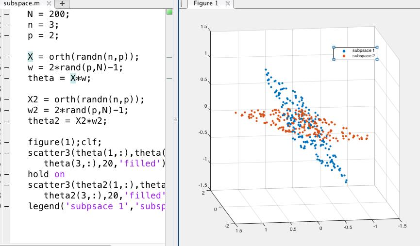
13 13 / 34

14 Examples Example: Constant subspace p = 1, X = x 1 = (1/ 1 n). R n 1 θ = x 1 w 1 is a constant signal with unknown amplitude. Example: Recommender system We have n movies in a database, and for a new client want to estimate how much they will like each movie, denoted θ R n. We have p existing archetype clients for whom we know their movie preferences; the preferences of the i th archetype client are denoted x i R n, i = 1,..., p. We will assume that θ is a weighted combination of these archetype profiles. 14 / 34

15 Example: Polynomial regression θ i = w 1 + w 2 i + w 3 i w p i p 1 X = Vandermonde matrix 15 / 34

16 Using subspace models Imagine we measure a function or signal in noise, y = θ + ν, where elements of ν are independent realizations from a Gaussian density and θ = Xw Question: How can we use knowledge of X to estimate θ from y? Let X be the subspace spanned by the columns of X, and let X be its orthogonal subspace. Then we can uniquely write y = u + v, where u X and v X. Since we know θ X, v can be considered pure noise and it makes sense to remove it. Answer: Orthogonal projection find the point in u X which is closest to the observed y. In general θ u because ν has some component in X. 16 / 34

17 Orthogonal projection Given a point y R n and subspace X, let s say we want to find the point ŷ X which is closest to y: ŷ = arg min θ y 2 θ X = arg min θ y 2 θ=xw,w Rp = arg min Xw y 2 θ=xw,w Rp = X (X X) 1 X y. }{{} pseudoinverse of X }{{} =:P X, projection matrix Essentially, we want to keep the component of y that lies in the subspace X and remove or kill the component in the orthogonal subspace. 17 / 34

18 Sinusoid subspace Example: Sinusoid subspace Let θ i = A cos(2πfi + φ), i = 1,..., n where frequency f is known but amplitude A and phase φ are unknown. Goal: estimate A and φ from where ν is white Gaussian noise. y = θ + ν First we need to express θ = [θ 1,..., θ n ] as an element in a 2-dimensional subspace; i.e. write θ = Xw where X is a known n 2 matrix and w is unknown. Then we can apply orthogonal projection. 18 / 34

19 Real solution: First note that cos(α + β) = cos(α) cos(β) sin(α) sin(β), so that θ i = A cos(2πfi + φ) = A cos(2πfi) cos(φ) A sin(2πfi) sin(φ). Let w 1 := A cos(φ) and w 2 := A sin(φ), and cos(2πf) sin(2πf) cos(4πf) sin(4πf) X =.. cos(2nπf) sin(2nπf). Note θ = Xw where X R n 2 and w R 2. Use pseudoinverse to compute ŵ, then set  = ŵ1 2 + ŵ2 2 φ = arctan( ŵ 2 /ŵ 1 ) 19 / 34

20 MLE and Linear Models When we observe y = θ + ν = Xw + ν and ν N (0, σ 2 I n ), then the MLE of w (and hence θ) can be computed by projection onto the subspace spanned by the columns of X. For more general probability models, the MLE may not have this form. Generalized linear models provide a unifying framework for modeling the relationship between y and w. The basic idea is that we define a link function g such that g(ey) = Xw. Typically there is no closed-form expression for ŵ MLE and it must be computed numerically. 20 / 34

21 Example: Colored Gaussian Noise y N (Xw, Σ), w R p, Σ, X known 1 p(y w) = (2π) n/2 Σ 1/2 exp{ 1 2 (y Xw) Σ 1 (y Xw)} The value of ŵ is given by, ŵ = arg min log p(y w) w = arg min (y w Xw) Σ 1 (y Xw) = (X Σ 1 X) 1 X Σ 1 y 21 / 34

22 Invariance of MLE Suppose we wish to estimate the function g = G(θ) and not θ itself. Intuitively we might try where θ is the MLE of θ. ĝ = G( θ) Remarkably, it turns out that ĝ is the MLE of g. This very special invariance principle is summarized in the following theorem. Theorem: Invariance of the MLE Let θ denote the MLE of θ. Then ĝ = G( θ) is the MLE of g = G(θ). 22 / 34

23 Example: Let y = [y 1,, y n ] where y i Poisson(λ). Given y, find the MLE of the probability that y Poisson(λ) exceeds the mean λ. G(λ) = P(y > λ) = λ λk e k! k= λ+1 ; z = largest integer z The MLE of g is ĝ = k= λ+1 λ λ k e k! where λ is the MLE of λ: λ = 1 n n i=1 y i 23 / 34

24 Sketch Proof: Define the induced log likelihood function: L(y g) max log p(y θ) θ:g(θ)=g Θ G g The MLE of g is ĝ = arg max L(y g) g = arg max g max θ:g(θ)=g log p(y θ) = G( θ), where θ = MLE of θ 24 / 34

25 Terminology in Estimation Theory Define ɛ( θ) := θ θ Recall that θ = θ(y) is a function of data = ɛ( θ) is a statistic! Mean Squared Error: Bias: Variance / Covariance: E[ɛ ɛ] := MSE( θ) Bias( θ) := E[ θ] θ Var( θ) := E[( θ E[ θ])( θ E[ θ]) ] 25 / 34

26 Bias-variance decomposition Key fact: Bias 2 ( θ) + Var( θ) = MSE[ θ] Bias 2 ( θ) + Var( θ) =(θ E[ θ]) 2 + E[ θ 2 ] (E[ θ]) 2 =θ 2 2θE[ θ] + (E[ θ]) 2 + E[ θ 2 ] (E[ θ]) 2 =E[ θ 2 ] 2θE[ θ] + θ 2 =E[ θ 2 ] 2θE[ θ] + E[θ 2 ] =E[ θ 2 2θ θ + θ 2 ] =E[( θ θ) 2 ] =MSE[ θ] 26 / 34

27 Asymptotics Estimators are often studied as a function of the number of observations: θ(y) = θ n where n = dim y θ is asymptotically unbiased if An estimator is consistent if lim Bias( θ n ) = 0 n lim MSE( θ n ) = 0 n A consistent estimator is at least asymptotically unbiased. Some estimators are unbiased, but inconsistent. The latter basically means that our estimation does not improve as the number of data increase. Inconsistent estimators can provide reasonable estimates when we have a small number of data. However, consistent estimators are usually favored in practice. 27 / 34

28 Estimator Accuracy Consider the likelihood function p(y θ) where θ is a scalar unknown (parameter). We can plot the likelihood as a function of the unknown. The more peaky or spiky the likelihood function, the easier it is to determine the unknown parameter. The peakiness is effectively measured by the negative of the second derivative of the log-likelihood at its peak. 28 / 34

29 Fisher Information In general, the curvature will depend on the observed data: 2 log p(y θ) θ 2 is a function of y Thus an average measure of curvature is more appropriate. [ 2 ] log p(y θ) E θ 2 The expectation averages out randomness due to the data and is a function of θ alone. Definition: Fisher Information [ ( ) ] log p(y θ) 2 [ 2 ] log p(y θ) I(θ) := E = E θ θ 2 is the Fisher Information. Here the derivative is evaluated at the true value of θ and the expectation is with respect to p(y θ). 29 / 34

30 Asymptotic Distribution of MLE Let y i iid pθ, i = 1,..., n, where θ R p, L n (θ) := n i=1 log p(y i θ) and θn = arg max θ L n (θ), assume Ln(θ) θ j and 2 L n(θ) [ θ j θ ] k condition E log p(y θ) θ exist for all j, k, and the regularity = 0 for all θ holds. Then θ n asymp. N (θ, n 1 I 1 (θ )) where I(θ ) is the Fisher-Information Matrix (FIM), whose elements are given by [ [I(θ 2 log p(y θ) ] θ=θ )] j,k = E θ j θ k 30 / 34

31 Regularity condition The regularity condition amounts to assuming that we can interchange order of differentiation and integration to compute [ log p(y θ) ] log p(y θ) E = θ θ=θ θ p(y θ )dx θ=θ 1 p(y θ) p(y θ) = p(y θ ) θ p(y θ )dx = θ=θ θ dx θ=θ = [ p(y θ)dx] θ θ=θ = 0, since p(y θ)dx = 1 for all θ and the derivative of a constant is 0. The last line, where integration and differentiation are interchanged, is only possible for regular likelihood functions. This is simply the Fundamental Theorem of Calculus applied to p(y θ). As long as p(y θ) is absolutely continuous w.r.t. Lebesgue measure (i.e., when the derivative is well-defined), this is possible. This is true for many distributions, but not true when the support of y depends on θ ( e.g. y Unif(0, θ)). 31 / 34

32 Note: E[ θ] θ Cov( θ) 1 n I 1 (θ ) θ is consistent and efficient asymptotically (i.e., asymptotically achieves CRLB) Example: y N (A 1 n 1, σ 2 I n ) θ = [A, σ 2 ] Â = 1 n y i N n s := i=1 i=1 σ 2 ) (A, σ2 n n (y i Â)2 χ 2 n 1 ( ) σ 2 σ 2 = s n 32 / 34

33 Example: (cont.) For large n, the CLT tells us that Therefore, Hence, χ 2 n N (n, 2n). s N (n 1, 2(n 1)) approximately distributed σ 2 = 1 n (y i n Â)2 = σ2 n s i=1 ( ) (n 1) N σ 2 2(n 1)σ4, n n 2 33 / 34

34 Example: (cont.) Moreover, for large n ] [ ] [ ] A A E [ θ = n 1 n σ2 σ 2 = θ [ ] σ 2 /n 0 = C θ 0 2(n 1)σ 4 n 2 [ σ 2 /n 0 0 2σ 4 n = I 1 (θ ) inverse Fisher Info. Matrix ] Hence, θ N (θ, I 1 (θ )) for large n 34 / 34