Econ671 Factor Models: Principal Components

Transcription

1 Econ671 Factor Models: Principal Components Jun YU April 8, 2016 Jun YU () Econ671 Factor Models: Principal Components April 8, / 59

2 Factor Models: Principal Components Learning Objectives 1. Show how models in finance have a factor structure interpretation. 2. Understand principal components. 3. Deriving and interpreting an eigen decomposition. 4. A factor model of the term structure of interest rates. Background Reading 1. Matrices, Handout on course website - especially the section on eigenvalues and eigenvectors. EViews Computer Files 1. yields_us.wf1 2. yields_us_loadings.wf1 3. capm.wf1 Jun YU () Econ671 Factor Models: Principal Components April 8, / 59

3 Introduction An important feature of many asset markets is that key variables (returns, yields, spreads etc) often display similar features. 1. Mean Asset markets tend to move together whereby the spreads between the key variables are stationary, even though these key variables may be nonstationary (cointegration). 2. Variance Periods of turbulence and tranquility tend to coincide across asset markets both locally and internationally, with the global financial crisis representing an example of synchronized turbulence. 3. Dynamics The dynamical behavior within classes of asset markets tend to exhibit very similar autocorrelation patterns. Jun YU () Econ671 Factor Models: Principal Components April 8, / 59

4 Introduction Example (Term Structure of Interest Rates) The term structure of interest rates is the relationship between the yields of a bond for differing maturities The Figure shows that U.S. Treasury yields (%p.a.) for maturities from 1mthh to 10yrs, tend to move together. YIELD_M1 YIELD_M3 YIELD_M YIELD_Y1 YIELD_Y2 YIELD_Y YIELD_Y5 YIELD_Y7 YIELD_Y Jun YU () Econ671 Factor Models: Principal Components April 8, / 59

5 Introduction Suggests that the time series characteristics of many financial variables can be summarized by a small set of factors. To formalise this model consider the following linear regression equation r i,t = α i + β i s t + u i,t where - r i,t is the return on the i th asset - s t is the factor (or set of factors) with parameters (vectors) α i, β i - u i,t is an unknown disturbance term representing idiosyncratic movements in r i,t. It is important to distinguish between two types of factors. 1. Observable s t 2. Unobservable s t Jun YU () Econ671 Factor Models: Principal Components April 8, / 59

6 Introduction 1. Observable s t Time series are available on s t, whereby the parameter β i is estimated simply by regressing r i,t on s t. Typical examples of this type of model are CAPM, and the Fama-French three-factor model. Example (CAPM) The CAPM r i,t r f,t = α i + β i (r m,t r f,t ) + u i,t is estimated for 6 assets using monthly data for the U.S. beginning May 1990 and ending July The OLS parameter estimates are summarised below. Asset: Exxon GE Gold IBM Microsoft Walmart α i : β i : Jun YU () Econ671 Factor Models: Principal Components April 8, / 59

7 Introduction 2. Unobservable s t Time series are not directly available on s t making the application of least squares to estimate α i and β i unworkable. There are two solutions: (a) Proxy variables A proxy variable is used instead of s t, but this creates errors in variables problems. In fact, this is a common strategy, if adopted only implicitly, with the application of the CAPM being a typical example. (b) Latent variables The statistical solution is to still treat s t as an unobservable variable, but to introduce additional structure on the model thereby providing additional information to enable the parameters to be estimated. This is the main focus of this and the next lecture! Jun YU () Econ671 Factor Models: Principal Components April 8, / 59

8 Introduction If s t is latent it is not immediately obvious how the parameters of r i,t = α i + β i s t + u i,t can be identified when all of the terms on the right hand-side of the equation (i) Parameters : α i, β i (ii) Explanatory variables : s t (iii) Disturbance term : u i,t are unknown. Two broad methods are investigated to show how to address this identification problem. 1. Principal Components (this lecture) 2. Kalman Filter (next lecture) Jun YU () Econ671 Factor Models: Principal Components April 8, / 59

9 The Role of Factors in Finance To motivate the role of factors in finance various models are presented, ranging from theoretical to purely statistical models. An important feature of this discussion is the distinction between factors that are observable and factors that are unobservable, that is latent. The examples consist of 1. Term Structure of Interest Rates 2. Capital Asset Pricing Model (CAPM) 3. Arbitrage Pricing Theory (APT) Jun YU () Econ671 Factor Models: Principal Components April 8, / 59

10 The Role of Factors in Finance Term Structure of Interest Rates Inspection of the U.S. Treasury yields (%p.a.) for maturities from 1 month to 10 years, reveals two important characteristics. 1. The levels of the yields tend to move together. 2. Neighboring yields move together more closely than yields with greater differences in maturities. This latter empirical property of yields is highlighted by the following correlation matrix. corr = 1-mth 3-mth 6-mth 1-yr 2-yrs 3-yrs 5-yrs 7-yrs 10-yrs Jun YU () Econ671 Factor Models: Principal Components April 8, / 59

11 The Role of Factors in Finance Term Structure of Interest Rates These two characteristics suggest that a potential model to explain the term structure of interest rates is given by at least a two-factor model r i,t = α i + β 1,i s 1,t + β 2,i s 2,t + u i,t, i = 1, 2,, 9, where u i,t is the disturbance term and s 1,t and s 2,t are the factors designed to Level factor (s 1,t ) : Slope factor (s 2,t ) : Capture the level of yields Capture the correlation between neighbouring yields As the two factors are implied by the data, they are latent factors. Jun YU () Econ671 Factor Models: Principal Components April 8, / 59

12 The Role of Factors in Finance Capital Asset Pricing Model The CAPM r i,t r f,t = α i + β i (r m,t r f,t ) + u i,t represents a single factor model given by the excess return on the market r m,t r f,t, where the (market) factor is observable. Extending the model to allow for other observable factors including Fama-French factors, momentum, liquidity etc, generates a multi-factor CAPM. From a theoretical point of view, the use of r m,t in the model actually serves as a proxy for the excess return on all invested wealth. As this is an unobservable variable, the excess return on the market portfolio, r m,t r f,t, is essentially serving as a proxy. This suggests that the more theoretically correct CAPM specification is r i,t r f,t = α i + β i s t + u i,t where s t is now a latent factor representing the excess return on all invested wealth. Jun YU () Econ671 Factor Models: Principal Components April 8, / 59

13 The Role of Factors in Finance Arbitrage Pricing Theory This is an alternative form of the CAPM equation where the (unknown) excess return on wealth is extended to the multi-factor version of the CAPM where all factors are unknown r i,t = α i + K j=1 β i,j s j,t + u i,t where there are K latent factors (s 1,t, s 2,t,, s K,t ) and as before u i,t is a disturbance term representing the idiosyncratic factor (risk). This is the arbitrage pricing model (APT) of Ross (1976). The factors and the disturbance term are assumed to have the following properties { 1 : j = k Factors : E [s j,t ] = 0, E [s j,t s k,t ] = { 0 : j = k σ 2 Disturbance : E [u i,t ] = 0, E [u i,t u k,t ] = i : i = k 0 : i = k Covariance : E [u i,t s j,t ] = 0 Jun YU () Econ671 Factor Models: Principal Components April 8, / 59

14 The Role of Factors in Finance Arbitrage Pricing Theory Historical Background: Stephen Ross (1943-) He is the inventor of Arbitrage Pricing Theory and also very well known for his work in finance including the CIR model of interest rates (he is the R ). Jun YU () Econ671 Factor Models: Principal Components April 8, / 59

15 The Role of Factors in Finance Arbitrage Pricing Theory These assumptions imply a decomposition of the covariance matrix of r t = {r 1,t, r 2,t,, r N,t }. In the case of a K = 1 factor model (let β i = β i,1 for simplicity of notation) r i,t = α i + β i s 1,t + u i,t the covariance matrix is of the form (see the next tutorial for the derivation of this result) β σ2 1 β 1 β 2 β 1 β N β 2 β 1 β 2 2 cov(r t ) = + σ2 2 β 2 β N..... β N β 1 β N β 2 β 2 N + σ2 N This result shows that the covariance matrix can be reorganized into a factor structure which may be more informative about the movements in returns. Jun YU () Econ671 Factor Models: Principal Components April 8, / 59

16 Principal Components Specification Consider the following model containing N asset returns r t = {r 1,t, r 2,t,, r N,t } and K N factors s t = {s 1,t, s 2,t,, s K,t } r 1,t r 2,t. α 1 α 2. = β 1,1 β 1,2 β 1,K β 2,1 β 2,2 β 2,K s 1,t s 2,t. + u 1,t u 2,t. r N,t α N β N,1 β N,2 β N,K s K,t u N,t or in matrix notation r t αµ = βs t + u t where - α is a (N 1) vector containing the means of r t. - s t is a (K 1) vector containing the factors. - β is a (N K ) matrix containing the factor loadings. - u t is a (N 1) vector of disturbances. Jun YU () Econ671 Factor Models: Principal Components April 8, / 59

17 Principal Components Specification The vector of latent factors and the disturbance vector have the properties E [u t ] = 0, E [ u t u t ] = Ω E [s t = 0, E [ s t s t ] = I, E [ s t u t ] = 0, where Ω is a (N N) covariance matrix. As E [s t ] = E [u t ] = 0, the mean of the returns is E [r t ] = E [µ + βs t + u t ] = µ + βe [s t ] + E [u t ] = µ The factor equation r t α = βs t + u t shows that r t α can be decomposed into a systematic component (βs t ) and an idiosyncratic component (u t ). Jun YU () Econ671 Factor Models: Principal Components April 8, / 59

18 Principal Components Specification Given the properties of s t and u t, the covariance structure of r t simplifies as cov (r t ) = E [ (r t α) (r t α) ] = E [ (βs t + u t ) (βs t + u t ) ] = βe [ s t s t ] β + βe [ s t u t ] [ + E ut s t ] β + E [ u t u t ] ββ = }{{} Systematic Risk + }{{} Ω Idiosyncratic Risk This equation shows that the covariance matrix can be decomposed in terms of two sources of factors/risks. 1. Systematic risk ( ββ ). 2. Idiosyncratic risk (Ω). Jun YU () Econ671 Factor Models: Principal Components April 8, / 59

19 Principal Components Specification In the special case where the number of variables matches the number of factors (N = K ), there is an exact decomposition of the covariance matrix of r t as Ω = 0 in this case, with the covariance matrix cov (r t ) reducing to cov (r t ) = ββ = β 1 β 1 + β 2 β 2 + β N β N An important property of principal components is that they exhibit the same features as this equation cov (r t ) = λ 1 P 1 P 1 + λ 2 P 2 P λ N P N P N where λ i is the i th eigenvalue with (N 1) orthonormal eigenvector P i, that is, P i P i = 1 and P i P j = 0, i = j. A comparison of these equations suggests that the loading parameter vector β i be chosen as β i = λ i P i, i = 1, 2,, N Jun YU () Econ671 Factor Models: Principal Components April 8, / 59

20 Principal Components Specification Now consider the N variances of r t = {r 1,t, r 2,t,, r N,t }, corresponding to the diagonal elements of cov (r t ) var (r 1,t ) var (r 2,t ). var (r N,t ) = λ 1 P 2 1,1 P 2 2,1. P 2 N,1 + λ 2 P 2 1,2 P 2 2,3. P 2 N,2 + + λ 1 P 2 1,N P 2 2,N. P 2 N,N Given that the eigenvectors are normalized as P i P i = 1, then the sum of the elements of each of the column vectors on the right hand-side all equal unity, that is P1,1 2 + P2 2,1 + + P2 N,1 = 1 P1,2 2 + P2 2,2 + + P2 N,2 = 1... P1,N 2 + P2 2,N + + P2 N,N = 1 Jun YU () Econ671 Factor Models: Principal Components April 8, / 59

21 Principal Components Specification Thus a measure of the total volatility of all asset returns N var (r i,t ) = var (r 1,t ) + var (r 2,t ) + + var (r N,t ) i=1 is achieved by combining all of the variance equations as N ( var (r i,t ) = λ 1 P 2 1,1 + P2, P 2 ) N,1 i=1 ( +λ 2 P 2 1,2 + P2, PN,2 2 ) ( + + λ N P 2 1,N + P2,N PN,N 2 ) Given the normalization of the eigenvectors, this equation simplifies to N N var (r i,t ) = λ 1 + λ λ N = λ i i=1 i=1 That is, the total volatility of all r t equals the sum of all eigenvalues. Jun YU () Econ671 Factor Models: Principal Components April 8, / 59

22 Principal Components Specification Instead of performing an eigen decomposition on the covariance matrix cov (r t ), to circumvent scaling issues when variables are measured in different units for example, the correlation matrix cor (r t ) can be used instead. In this case as the correlation matrix contains unity on the main diagonal by definition, then the sum of correlations becomes N λ i = N i=1 By inspecting the relative magnitude of the largest eigenvalues it is possible to quantify the proportion of the total variance of the data that is explained by K < N principal components. Bai and Ng (2002, Econometrica) propose a formal test of the number of factors based on information criteria. Jun YU () Econ671 Factor Models: Principal Components April 8, / 59

23 The Role of Factors in Finance Specification Historical Background: Karl Pearson ( ) Inventor of Principal Components plus many other well-used and well-loved statistical techniques. Jun YU () Econ671 Factor Models: Principal Components April 8, / 59

24 Principal Components Estimation In practice it is necessary to estimate the eigenvalues and the eigenvectors from the data. As an example consider the following correlation matrix of the 1-month, 1-year and 5-year U.S. Treasury yields given earlier cor (r t ) = The EViews commands to estimate the eigenvalues and eigenvectors of cor (r t ), highlight the 3 series and double click the shaded region and then click Open Group / View / Principal Components... / Calculation For Type: choose Correlation / OK The output is given in the following window. Jun YU () Econ671 Factor Models: Principal Components April 8, / 59

25 Principal Components Estimation Source: EViews yields_us.wf1 Jun YU () Econ671 Factor Models: Principal Components April 8, / 59

26 Principal Components Estimation The estimated eigenvalues and eigenvectors of the correlation matrix are respectively λ = 0.151, P = with the columns of P representing the three eigenvectors P 1 = 0.588, P 2 = 0.299, P 3 = corresponding to the order of the three eigenvalues in λ. The use of the ^ emphasises that the population parameters λ and P are estimated from the data. Jun YU () Econ671 Factor Models: Principal Components April 8, / 59,

27 Principal Components Estimation Recovering the Correlation Matrix from the Decomposition The correlation matrix is recovered as follows: 1. Diagonal elements (ie own correlations) cor (r 1,t ) = (0.581) ( 0.490) (0.649) 2 = cor (r 2,t ) = (0.588) ( 0.299) ( 0.752) 2 = cor (r 3,t ) = (0.563) (0.819) (0.144) 2 = Jun YU () Econ671 Factor Models: Principal Components April 8, / 59

28 Principal Components Estimation 2. Off-diagonal elements cor (r 1,t, r 2,t ) = (0.581) (0.588) ( 0.490) ( 0.299) (0.649) ( 0.752) = cor (r 1,t, r 3,t ) = (0.581) (0.563) ( 0.490) (0.819) (0.649) (0.144) = cor (r 2,t, r 3,t ) = (0.588) (0.563) ( 0.299) (0.819) ( 0.752) (0.144) = Jun YU () Econ671 Factor Models: Principal Components April 8, / 59

29 Principal Components Estimation Properties of the Estimates Some key properties of the parameter estimates are as follows. 1. Normalization of eigenvectors = ( 0.490) 2 + ( 0.299) = Orthogonality of eigenvectors ( 0.752) = P 1 P 2 = ( 0.490) ( 0.299) = 0 P 1 P 3 = ( 0.752) = 0 P 2 P 3 = ( 0.490) (0.649) + ( 0.299) ( 0.752) = 0 Jun YU () Econ671 Factor Models: Principal Components April 8, / 59

30 Principal Components Estimation 3. Eigenvalues As it is the correlation matrix that is being used in the eigen decomposition, the eigenvalues sum to N = 3 The normalized eigenvalues are λ i = = 3 i = = = 1 The first eigenvalue explains 94.6% of the total variance, the second explains an additional 5%, while the contribution of the third and last eigenvalue is 0.4%. Jun YU () Econ671 Factor Models: Principal Components April 8, / 59

31 Principal Components Estimation 4. Factor loadings β 1 = λ 1 P 1 = = β 2 = λ 2 P 2 = = β 3 = λ 3 P 3 = = Intercepts As E [r t ] = α, an estimate of α is given by the sample mean of r t given by α = r = [ ] Jun YU () Econ671 Factor Models: Principal Components April 8, / 59

32 Principal Components Estimation The K = 1 Estimated Factor Model The estimated model is r 1,t = α 1 + β 1,1 s 1,t + û 1,t = s 1,t + û 1,t r 2,t = α 2 + β 2,1 s 1,t + û 2,t = s 1,t + û 3,t r 3,t = α 3 + β 3,1 s 1,t + û 3,t = s 1,t + û 3,t An increase in the factor s 1,t, results in all 3 yields increasing by similar amounts. This suggests that s 1,t is a LEVEL factor. Jun YU () Econ671 Factor Models: Principal Components April 8, / 59

33 Principal Components Estimation As E [ s1,t 2 ] = 1, the systematic risks are ĥ 1 = β 2 1,1 = = ĥ 2 = β 2 2,1 = = ĥ 3 = β 2 3,1 = = The idiosyncratic risks are var (û 1,t ) = var (r 1,t ) ĥ 1,t = = var (û 2,t ) = var (r 2,t ) ĥ 2,t = = var (û 3,t ) = var (r 3,t ) ĥ 3,t = = Jun YU () Econ671 Factor Models: Principal Components April 8, / 59

34 Principal Components Estimation The K = 2 Estimated Factor Model The estimated model is r 1,t = s 1,t 0.190s 2,t + û 1,t r 2,t = s 1,t 0.116s 2,t + û 2,t r 3,t = s 1,t s 2,t + û 3,t An increase in the factor s 2,t, widens the spreads between all 3 yields as r 1,t falls, as does r 2,t but by a smaller amount, whilst r 3,t increases. This suggests that s 2,t is a SLOPE factor as it changes the slope of the yield curve. Jun YU () Econ671 Factor Models: Principal Components April 8, / 59

35 Principal Components Estimation As E [ s1,t 2 ] [ ] = E s 2 2,t = 1, the systematic risks are ĥ 1 = β 2 1,1 + β 2 1,2 = ( 0.190) 2 = ĥ 2 = β 2 2,1 + β 2 2,2 = ( 0.116) 2 = ĥ 3 = β 2 3,1 + β 2 3,2 = = The idiosyncratic risks are var (û 1,t ) = var (r 1,t ) ĥ 1 = = var (û 2,t ) = var (r 2,t ) ĥ 2 = = var (û 3,t ) = var (r 3,t ) ĥ 3 = = Jun YU () Econ671 Factor Models: Principal Components April 8, / 59

36 Principal Components Estimation The K = 3 Estimated Factor Model The estimated model is r 1,t = s 1,t 0.190s 2,t s 3,t r 2,t = s 1,t 0.116s 2,t 0.082s 3,t r 3,t = s 1,t s 2,t s 3,t. There are no idiosyncratic terms in this model as 3 factors perfectly explain the movements of the 3 interest rates. Nonetheless it is sometimes hard to diversify all latent factors! Jun YU () Econ671 Factor Models: Principal Components April 8, / 59

37 Principal Components Estimation As E [ s 2 1,t ] = E [ s 2 2,t ] = E [ s 2 3,t ] = 1, the systematic risks now equal the diagonal components of the correlation matrix as ĥ 1 = β 2 1,1 + β 2 1,2 + β 2 1,3 = ( 0.190) = ĥ 2 = β 2 2,1 + β 2 2,2 + β 2 2,3 = ( 0.116) 2 + ( 0.082) 2 = ĥ 3 = β 2 3,1 + β 2 3,2 + β 2 3,3 = = In which case the idiosyncratic risks are all zero var (û 1,t ) = var (r 1,t ) ĥ 1 = = var (û 2,t ) = var (r 2,t ) ĥ 2 = = var (û 3,t ) = var (r 3,t ) ĥ 3 = = Jun YU () Econ671 Factor Models: Principal Components April 8, / 59

38 Principal Components Factor Extraction Method Since r i,t = α i + β i s 1,t + u i,t, i = 1,..., N, having estimated the factor model, estimates of the vector of factor loadings at time t are obtained as ŝ t = ( β Ω 1 β) 1 β Ω 1 (r t µ) where ŝ t is a (K 1) vector of the estimated factors at time t, β is a (N K ) estimated matrix of factor loadings, Ω is the (N N) covariance matrix of û t, r t is a (N 1) vector of interest rates and µ is a (N 1) vector of sample means corresponding to the vector of interest rates. Jun YU () Econ671 Factor Models: Principal Components April 8, / 59

39 Principal Components Factor Extraction If Ω = σ 2 I, K = 1, then ŝ t = N β i=1 i (r it µ i ). The bigger the factor N i=1 β 2 i loading, the more importance of the variable in determining the factor. This expression shows that the factors at time t are a (weighted) linear function of the actual interest rates at time t. Jun YU () Econ671 Factor Models: Principal Components April 8, / 59

40 Principal Components Factor Extraction EViews Commands The EViews commands to extract the factors, highlight the 3 series and double click the shaded region and then click Open Group / Proc / Make Principal Components... For Scores series names:, write in the window Level Slope Curvature Then click Calculation and for Type: choose Correlation / OK The output will be presented in a spreadsheet. Jun YU () Econ671 Factor Models: Principal Components April 8, / 59

41 Principal Components Factor Extraction Interpretation The three factors are plotted over time. 4 3 LEVEL SLOPE CURVATURE Source: EViews file yields_us.wf1 The results show that: (i) The LEVEL factor dominates the SLOPE and CURVATURE factors. (ii) As the LEVEL factor tracks the three yields this suggests that a 1-factor model suffi ces to explain the three yields. Jun YU () Econ671 Factor Models: Principal Components April 8, / 59

42 A Multi-Factor Model of Interest Rates Consider the N = 9, U.S. Treasury yields (percentage, annualized) from July 2001 to September 2010, presented in the Figure earlier. The N = 9 eigenvalues of the correlation matrix from highest to lowest are λ = {8.2339, , , , , , , , } The proportionate contributions of the first three eigenvalues are λ 1 = = 0.915, λ 2 = = 0.079, λ 3 = This suggest that a K = 3 factor model explains the U.S. term structure with the first three eigenvalues explaining = 0.999, or 99.9% of the total variance/correlation in the yields. = Jun YU () Econ671 Factor Models: Principal Components April 8, / 59

43 A Multi-Factor Model of Interest Rates The estimated factor loadings on the first factor are computed as β 1,1 β 2,1 β 3,1 β 4,1 β 5,1 β 6,1 β 7,1 β 8,1 β 9,1 = = The other factor loadings are computed in a similar way. Jun YU () Econ671 Factor Models: Principal Components April 8, / 59

44 A Multi-Factor Model of Interest Rates The following Figure plots the loadings of the first three factors which are identified respectively as level, slope and curvature LEVEL SLOPE CURVATURE Source: EViews file yields_us.wf1 Jun YU () Econ671 Factor Models: Principal Components April 8, / 59

45 A Multi-Factor Model of Interest Rates Factor Interpretation 1. Level Factor The first factor represents a levels effect as a shock to this factor raises all yields by approximately the same amount. 2. Slope Factor The second factor is a slope factor as a positive shock twists the yield curve by lowering short rates (negative loadings) and raising long rates (positive loadings). 3. Curvature Factor The third factor is a curvature factor which bends the yield curve by simultaneously raising the very short and long rates (positive loadings), while lowering (negative loadings) the intermediate rates at around 2 years (24 months) and 3 years (36 months). Jun YU () Econ671 Factor Models: Principal Components April 8, / 59

46 A Multi-Factor Model of Interest Rates The three factors are plotted over time LEVEL SLOPE CURVATURE During the recent crisis: Source: EViews file yields_us.wf1 (i) The LEVEL factor falls showing that all yields were falling. (ii) The SLOPE factor becomes negative suggesting an inverted yield curve. (iii) The CURVATURE factor becomes negative at the end of 2008, suggesting that short and long yields fall relative to intermediate yields. Jun YU () Econ671 Factor Models: Principal Components April 8, / 59

47 A Latent Factor CAPM The latent multi-factor CAPM is r i,t r f,t = α i + K j=1 β i,j s j,t + u i,t where s j,t are unobserved latent factors. The data are the excess returns on 6 stocks consisting of Exxon, GE, Gold, IBM, Microsoft and Walmart. The data are monthly beginning in April 1990 and ending in July The covariance matrix is cov (r t ) = Jun YU () Econ671 Factor Models: Principal Components April 8, / 59

48 A Latent Factor CAPM The EViews output from the principal components decomposition based on the covariance matrix is Source: EViews file capm.wf1 Jun YU () Econ671 Factor Models: Principal Components April 8, / 59

49 A Latent Factor CAPM The N = 6 eigenvalues of the covariance matrix from highest to lowest are λ = { , , , , , } The total sum of the eigenvalues is = This sum equals the total volatility of all 6 excess returns as given by the sum of their variances = Jun YU () Econ671 Factor Models: Principal Components April 8, / 59

50 A Latent Factor CAPM The proportionate contributions of the first three eigenvalues to total volatility are λ 1 = = λ 2 = = λ 3 = = The first factor explains 51.27% of total volatility (equal to ). - The second factor explains 17.30% of total volatility. - The third factor explains 13.98% of volatility. So the first three factors explain jointly = or 82.55% of total volatility. This suggests that a 1-factor CAPM is potentially inappropriate and there is a need for a 3-factor model (maybe even higher). Jun YU () Econ671 Factor Models: Principal Components April 8, / 59

51 A Latent Factor CAPM To estimate the multi-factor CAPM, the intercepts (α i ) are estimated using the sample means as given by the EViews output. Source: EViews file capm.wf1 Jun YU () Econ671 Factor Models: Principal Components April 8, / 59

52 A Latent Factor CAPM Using the first eigen vector, the K = 1 factor CAPM is estimated as β 1 = λ 1 P 1 = These results show that = (i) Gold moves in the opposite direction to the other assets, which is consistent with the asset representing a hedge stock. (ii) Microsoft has the highest loading, equal to , showing that this asset responds the most to changes in the factor s 1,t, compared to the other stocks. This result is consistent with Microsoft being an aggressive stock at least relative to the other stocks. Jun YU () Econ671 Factor Models: Principal Components April 8, / 59

53 A Latent Factor CAPM Using the sample means and the loadings on the first factor, the estimated K = 1 factor model is then Exxon : r 1,t = s 1,t + û 1,t GE : r 2,t = s 1,t + û 2,t Gold : r 3,t = s 1,t + û 3,t IBM : r 4,t = s 1,t + û 4,t Microsoft : r 5,t = s 1,t + û 5,t Walmart : r 6,t = s 1,t + û 6,t For comparison the OLS estimates of the CAPM with the excess return on the market as the (observable) factor are given below. The beta-risk estimates are very different from the two models. Part of the reason for this is that the variance of s 1,t by construction is normalized to be unity, whereas the variance of the excess return on the market r m,t r f,t, is not. Jun YU () Econ671 Factor Models: Principal Components April 8, / 59

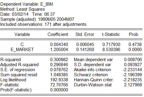
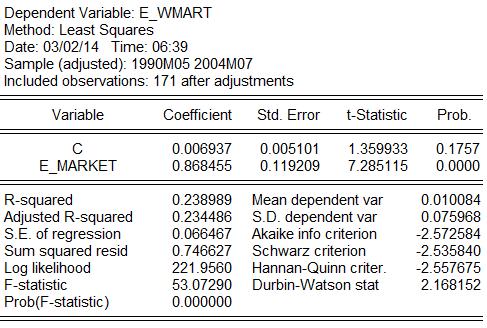
54 A Latent Factor CAPM Jun YU () Econ671 Factor Models: Principal Components April 8, / 59

55 A Latent Factor CAPM To make the beta-risk estimates commensurate across the two estimated models the approach is to rescale s 1,t to make it equivalent to the variance of r m,t r f,t. The EViews output of the descriptive statistics of r m,t r f,t shows that the variance is var (r m,t r f,t ) = Series: E_MARKET Sample 1990M M07 Observations 171 Mean Median Maximum Minimum Std. Dev Skewness Kurtosis Jarque Bera Probability Source: EViews file capm.wf1 Jun YU () Econ671 Factor Models: Principal Components April 8, / 59

56 A Latent Factor CAPM Reconsider the 1-factor CAPM r i,t r f,t = α i + β i,1 s 1,t + u i,t Defining σ m as the standard deviation of the excess return on the market, then the model is rewritten as r i,t r f,t = α i + β i,1 σ m σ m s 1,t + u i,t = α i + β i,1 σ m (σ m s 1,t ) + u i,t Here the factor know has a variance equal to the variance of the excess return on the market as [ E (σ m s 1,t ) 2] = σ 2 me [ s1,t 2 ] = σ 2 m 1 = σ 2 m Thus, the rescaled beta-risk estimates are obtained by dividing the loading vector β i,1, by the standard deviation of σ m = r m,t r f,t. Jun YU () Econ671 Factor Models: Principal Components April 8, / 59

57 These rescaled beta estimates are β 1 = β = Interpretation: / / / / / / = (i) GE tracks the market with a beta-risk of (ii) Exxon and Walmart are conservative stocks with estimates between 0 and 1. (iii) The tech-stocks of IBM and Microsoft are aggressive stocks with estimates greater than 1. (iv) Gold is a hedge stock with a beta-risk of Jun YU () Econ671 Factor Models: Principal Components April 8, / 59

58 A Latent Factor CAPM The estimate of the first factor (ŝ 1,t ) is plotted over time (note that the two factors are not scaled to have the same variances) S1T E_MARKET Source: EViews file capm.wf1 These results show that there are some similarities in the two factors as well as some differences. The correlation between the two factors is showing that the first factor is highly correlated with the excess returns on the market. Jun YU () Econ671 Factor Models: Principal Components April 8, / 59

59 End of Lecture Jun YU () Econ671 Factor Models: Principal Components April 8, / 59