A probabilistic description of the bed load sediment flux: 2. Particle activity and motions

Transcription

1 A probabilistic description of the bed load sediment flux: 2. Particle activity and motions John C. Roseberry, Mark W. Schmeeckle, and David Jon Furbish 1 Department of Earth and Environmental Sciences and Department of Civil and Environmental Engineering, Vanderbilt University, Nashville, Tennessee, USA. 2 School of Geographical Sciences, Arizona State University, Tempe, Arizona, USA. Abstract. High-speed imaging of coarse sand particles transported as bed load over a planar bed reveals that the particle activity, the solid volume of particles in motion per unit streambed area, fluctuates as particles respond to near-bed fluid turbulence while simultaneously interacting with the bed. The relative magnitude of these fluctuations systematically varies with the size of the sampling area. The particle activity within a specified sampling area is distributed in a manner that is consistent with the existence of an ensemble of configurations of particle positions wherein certain configurations are preferentially selected or excluded by the turbulence structure, manifest as patchiness of active particles. The particle activity increases with increasing bed stress far faster than does the average particle velocity, so changes in the transport rate with changing stress are dominated by changes in the activity, not velocity. The probability density functions of the streamwise and cross-stream particle velocities are exponential-like and lack heavy tails. Einstein-Smoluchowsky-like relations of the mean squared displacement versus time may ostensibly indicate non-fickian behavior while actually reflecting effects of correlated random walks associated with intrinsic periodicities in particle motions, not anomalous diffusion. The probability density functions of the particle hop distance (start-tostop) and the associated travel time are gamma-like, which provides the empirical basis for showing that particle disentrainment rates vary with hop distance and travel time. 1. Introduction At any instant the solid volume of bed load particles in motion per unit area of streambed, the particle activity [L], can vary temporally and spatially due to short-lived near-bed turbulence excursions as well as longer-lived influences of bed form geometry on the mean flow [Drake et al., 1988; McLean et al., 1994; Nelson et al., 1995; Schmeeckle and Nelson, 2003; Singh et al., 2009; Furbish and Schmeeckle, 2011]. The activity also varies as particles alternate between states of motion and rest over a large range of timescales. During their motions, particles respond to near-bed fluid motions and interact with the bed so that, at any instant within a given small area, some particles move faster and some move slower than the average within the area. Particles within a specified streambed area therefore possess at any instant a distribution of velocities. As described in companion papers [Furbish et al., 2012a, 2012b], these two components of bed load particle 1

2 motions the particle activity and the particle velocity distribution figure prominently in describing the rate of sediment transport and the rate of dispersal of particles during transport. Specifically, the bed load particle flux involves an advective part consisting of the product of the particle activity and the mean velocity, as is normally assumed, but more generally it also involves a diffusive part associated with spatial variations in the particle activity and velocity [Lisle et al., 1998; Schmeeckle and Furbish, 2007; Furbish et al, 2009a, 2009b; Furbish et al., 2012a]. The purpose of this paper is to provide tangible experimental measurements of key features of the particle activity and particle motions that bear on the bed load sediment flux and sediment particle diffusion. We describe results from experiments, initially reported by Schmeeckle and Furbish [2007], involving high-speed imaging of coarse sand particles transported as bed load over a planar bed. The imaged time series of particle motions, as in similar experiments described by Lajeunesse et al. [2010], reveal important features of both individual particle motions and the collective behavior of these motions. With respect to particle activity the experimental time series reveal that: (i) the activity fluctuates as particles respond to near-bed fluid turbulence while simultaneously interacting with the bed, where the magnitude of the fluctuations in activity relative to the overall level of activity depends 2 on the size of the sampling area; (ii) the activity within a specified sampling area db [L ] is distributed in a manner that is consistent with the existence of an ensemble of configurations of 2 particle positions over a larger area B [L ], wherein certain configurations are preferentially selected or excluded by the turbulence structure [Furbish et al., 2012a]; and (iii) the activity increases with increasing bed stress faster than does the average particle velocity [Schmeeckle and Furbish, 2007; Ancey, 2010; Lajeunesse et al., 2010], which bears on conceptualizing stress-based formulations of sediment transport. With respect to particle motions: (i) the probability density functions, 2 [L t] and [L t], of the streamwise and cross-stream particle velocities, u p[l t ] and v p[l t ], are exponentiallike, consistent with the experimental results of Lajeunesse et al. [2010]; (ii) measures of the particle 2 diffusivity [L t ], notably the Einstein-Smoluchowsky and related equations, may ostensibly indicate non-fickian behavior while actually reflecting effects of correlated random walks [e.g. Viswanathan et al., 2005] associated with intrinsic periodicities in particle motions, not anomalous diffusion; and (iii) the probability density functions of the particle hop distance [L] (start-to-stop) and the associated travel time [t] are gamma-like, which provides the empirical basis for showing that the spatial and temporal rates of particle disentrainment vary with and [Furbish and Haff, 2010; Furbish et al., 2012a]. These experimental results thereby illustrate key probabilistic elements of the bed load sediment flux as described by Furbish et al. [2012a]. Moreover, the results form the basis of the analysis presented in the third paper of this series [Furbish et al., 2012b], which describes what the particle velocity distributions and reveal about how particle momenta vary as particles accelerate and decelerate between entrainment and disentrainment in response to fluid drag and interactions with the bed. In addition, the results form the basis of a proof-of-concept [Furbish et al., 2012c; Ball, 2012] that G. I. Taylor s classic formulation of diffusion of continuous motions [Taylor, 1921] yields a proper description of diffusion of bed load particles at low transport rates, consistent with Fickian diffusion. This paper involves an unusually rich data set. In order to present the material within limited space we have necessarily selected a few of many possible example data for the figures, with the intention of fairly representing the full range of conditions in our experiments. [Note: Although not yet accepted for publication, the companion papers Furbish et al. [2012a, 2012b, 2012c] are cited

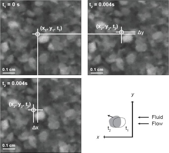
3 with a 2012 date for simplicity of reference.] 2. Laboratory Experiments and Measurements Experiments were conducted with an 8.5 m 0.3 m flume in the River Dynamics Laboratory at Arizona State University. For several flow conditions (Table 1), fluid velocities were measured with an acoustic doppler velocimeter (ADV) at a position one cm above the bed surface, from which bed shear stresses were calculated using the logarithmic law of the wall and a value of the roughness length z 0 [L] equal to D 50/30. Bed material consisted of relatively uniform coarse sand with an average diameter D 50 of 0.05 cm. The bed was smoothed before each experiment. High-speed imaging at 250 frames per second over a 7.57 cm (streamwise) by 6.05 cm (cross-stream) bedsurface domain with 1,280 1,024 pixel resolution provided the basis for tracking particle motions. A small plexiglass sled window was placed on the water surface so that the camera had a clear view of the bed surface through the water column without effects of image distortion by light refraction with water-surface undulations. Flow depths were sufficiently large that the window did not interfere with the flow at the bed surface in the area filmed. The image series involved a duration of seconds (4,912 frames) for each of the four stress conditions. We then performed two sets of measurements. In the first set, designated as A, we used runs R1, R2, R3 and R5 to track all active particles within a specified window at one of two sampling intervals over varying time durations (Table 1). In the second set of measurements, designated as B, we used runs R2 and R3 to track virtually all active particles over the full 1,280 1,024 pixel domain using a frame interval of sec over a shorter duration (0.4 sec). The four series in set A provide a description of particle activities and velocities, and fluctuations in these quantities, over durations much longer than the average particle hop time. The two series in set B, although of shorter duration, provide a detailed description of particle motions over the full image domain at a finer resolution than that provided in set A. For set A, we used ImageJ (an open source code available from the National Institutes of Health) to mark the centroid of each active particle as it moved within successive frames, recording the centroid pixel coordinates. These were converted to streamwise and cross-stream coordinate positions, x p[l] and y p[l]. For set B, images were imported into ArcGIS 9.3 and spatial coordinates were edited as a point shapefile. For each particle in motion we located the intersection of lines tangent to its leading edge and its top or bottom edge in each frame to specify its (x p, y p) position (Figure 1). All particles that visibly moved over the entire duration of video R2B were tracked, giving 870 unique spatial coordinates from 20 particles. In video R3B, the spatial coordinates of approximately 95% of all particles in motion were tracked, giving over 13,000 spatial positions from 311 particles. The particles not tracked in R3B were those whose identities were too difficult to maintain through the video or that exited the field of view early, or entered the field of view late. This particle tracking method allows for resolution of sub-pixel motions through observing a particle over successive frames such that its position can be interpolated between frames. To wit, changes in the grayscale pixel values of a tracked particle are indicative of its sub-pixel motion within the context of previous motion over several pixels. Particles that slightly rocked back and forth in a pocket, but otherwise did not move ( hop ), were not included in the dataset. To maintain consistency, all particle locations were identified by one person (JCR). Although this method is time consuming, it includes the smallest measurable particle displacements without bias toward an overrepresentation of these small displacements, and it provides a virtually complete collection of the positions of moving particles. For both sets of measurements (A and B), we calculated the streamwise and cross-stream particle 3

4 displacements r = x p(t + t) - x p(t) [L] and s = y p(t + t) - y p(t) [L] between frames, and from these we estimated the instantaneous particle velocity components u p= r/ t [L t ] and v p= s/ t [L t ], where t [t] is the selected sampling interval (0.012 sec for R1, R2; sec for R3, R5, R2B, R3B). These paired velocity components involved numerous instants with v p = 0 and finite u p, and fewer instants with u p= 0 and finite v p. Although particles mostly moved downstream, some particles occasionally moved upstream (u p < 0). We considered a particle with u p = v p = 0 to be at rest, even if for only one frame interval. Conversely, a particle is considered to be active if either u or v is finite. p p 3. Particle Activity and Motions 3.1. Variations in Particle Activity The particle activity (t) varies with position and time within the experimental domain B depending on the bed stress and the size of the sampling area db. To illustrate this we divide the domain B into four sets of m partitions, each partition of size db = B/m. Specifically, a partitioning of B into 8, 4, 2 and 1 units coincides respectively with db equal to 5.7 cm, 11.4 cm, 22.9 cm and cm (Figure 2). For the two experiments (R2B, R3B) in which we measured essentially all active particles, we plot the time series of particle number activity n(t; db) = (t; db)/v p, that is, the 3 number of particles per area db (Figure 3), where V p [L ] is the particle volume. At any instant, the activity n(t; db) varies from one area db to the next; and over time the particle activity n(t; db) varies within each area db (Figures 2 and 3). There is a weak correlation in the activity between upstream and downstream areas db, offset by the travel time of particles between adjacent areas, illustrating the presence of turbulent sweeps interacting with the sediment surface. However, this is not simply a streamwise translation of particle activity as turbulent sweeps progress downstream. Simultaneously, spatial variations in entrainment and disentrainment of particles contribute to the variability in n(t; db) [Drake et al., 1988]. For example, with two partitions of R3B (Figure 3), an increase in particle activity for the entire area begins around t = 0.24 sec. The peak in activity for the downstream area (B) associated with this overall increase occurs nearly 0.1 sec after the peak of the upstream area (A), which occurs shortly after t = 0.24 sec. Thus the total activity, which is the average over both partitions, has a peak between those of area A and B. For a given bed stress and associated mean particle activity, the temporal variability in the activity decreases with increasing area db (Figure 4) as the number N a of active particles on average increases, and fluctuations associated with deposition and entrainment within db proportionally decrease relative to the overall activity n(t; db). For the same reason, the variability in particle activity for any area db decreases with increasing bed stress. Autocorrelation functions r n(k) of the particle activity reveal key features of the temporal variability in the activity. Each of these functions in set A exhibits a quasi-periodic structure (Figure 5) that reflects the response in particle activity to turbulent sweep events (visible in the videos) at varying timescales. The primary periodicity varies from one to two seconds. In all cases, r n(k) decays (initially) to zero in one second or less, and both R1 and R5 exhibit a quasi-periodic structure over periods less than one second. In turn, the functions r n(k) based on the shorter series of R2B and R3B exhibit this sub-second quasi-periodic structure, decaying to zero in less than 0.1 second, which roughly equals the average travel time of ~0.09 sec for particles in R3B. This autocorrelation structure indicates a strong coupling between particle activity (entrainment) and fluid motions, with rapid dampening of the activity (disentrainment) by frictional effects of particle-bed interactions Probability Distributions of Particle Activity 4

5 In each of our experiments the measurement window size db is such that the number of particles within db, as described above, varies over time (from frame to frame). Here we assume for illustration that the time realization (frames) in each experiment provides a representative sample of the possible numbers of particles within db, and that there exists a total number N a of active particles distributed over a larger area B in each of an ensemble of possible configurations of particle positions [Furbish et al., 2012a]. In effect we swap time realizations for ensemble realizations. Focusing on the set A experiments, if n db denotes the number of active particles within a sampling window of area db, then the discrete probability density function P n(n db) introduced by Furbish et al. [2012a, Appendix C therein] reveals that the number of particles n db is distributed in a manner where certain configurations are preferentially selected or excluded by the turbulence structure depending on the transport stage. To illustrate this point we first set up the null hypothesis that each configuration is equally probable, which leads to the corollary that particle positions are entirely spatially random. Namely, if N a is the total number of active particles in each possible configuration of the ensemble of configurations of particle positions over a total streambed area B, and if m denotes the number of partitions of B of area db = B/m, then the total number of configurations involving N particles distributed among m partitions is a (1) Using the language of statistical mechanics, we may refer to each of these N e configurations as a macrostate. In turn, if n 1, n 2, n 3,..., n m denote the number of particles in each of the m partitions of an individual macrostate, then using Maxwell-Boltzmann counting there are n e ways in which the N a particles may be interchanged amongst the m partitions, and we may refer to each of these ne arrangements as a microstate. The number of microstates in a given macrostate is (2) In turn, the discrete probability density function of n 1, n 2,..., n m is given by the multinomial distribution, where p 1, p 1, p 3,... p m denote the probabilities that a particle will be positioned within each of the m partitions. We may now simplify as follows. Of interest is the distribution of the number of particles n = n db within one partition of area db. A particle is either within or outside of this partition, so effectively there are two partitions and (3) reduces to the binomial distribution, (3) (4) For comparison with our data (Figure 6), we approximate P n(n db) as a Poisson distribution assuming large N a, which is equivalent to assuming that db B. This requires specifying only the expected (average) number of particles within db, estimated directly from the data. In addition, for illustration we use a simple Monte Carlo analysis to estimate the fifth and ninety-fifth percentiles 5

6 about the expected values of P n(n db) assuming a sample size of 200. (Our sample size is larger than this, but particle configurations are correlated in time. Because the particle activity becomes decorrelated by about 0.1 sec, and because the runs were almost 20 sec, 200 is a conservative estimate.) For R1, the fit between computed and observed values of P n(n db) is reasonably good, and we cannot reject the null hypothesis that particles are entirely randomly distributed. At higher transport stages (R2, R3 and R5), both small and large numbers ndb are observed in greater proportions than what is expected assuming spatial randomness. Thus, among the ensemble of possible configurations of particle positions and velocities, some configurations (as defined by Maxwell-Boltzmann counting) may be preferentially selected or excluded by the near-bed turbulence structure inasmuch as turbulent sweeps and bursts characteristically lead to patchy, fasta active particles are moving clouds of particles, or because unusual configurations (e.g. all N clustered within db or are distributed evenly over all partitions) are excluded by the physics of coupled fluid-particle motions [Furbish et al., 2012a]. That is, with particle clustering associated with sweeps (Figure 2), there is a higher probability of occurrence of large numbers of particles within an area db than what is predicted by the hypothesis of spatially random configurations arising from the assumption of equally probable microstates. (Likewise, there is a higher probability of occurrence of small numbers with the concomitant existence of inter-cluster areas.) Nonetheless, of particular significance is that these empirical results are consistent with the idea that there exists an imagined set (ensemble) of configurations of active article positions over an area B, which, under an appropriate assumption concerning the likely occurrence of each configuration (whether equally probable or weighted according to turbulence structure), directly yields the distribution of activity P (ndb) for an area db. n 3.3. Particle Trajectories and Velocities Most particles move downstream with a small component of cross-stream motion. Occasionally, small upstream displacements occur, mostly at low velocity when particles rotate out of pockets or move around stationary particles. Although upstream motions occur with disentrainment, these motions more typically are associated with particle entrainment. Focusing on results from R2B and R3B, entrainment and disentrainment occur both abruptly and gradually (Figure 7). Particle velocities in the final few hundredths of a second preceding deposition are on average greater than particle velocities during the same time frame immediately following entrainment. Thus, on average the magnitude of acceleration during entrainment is less than that during disentrainment. Whereas most particles immediately following entrainment or preceding deposition are at low velocities, there is a small but significant number of particles at relatively high velocity in the first or last ~ sec of motion [Ball, 2012; Furbish et al., 2012c] Particle velocities fluctuate at several timescales. Most basically, because particles start and stop, the velocity of each particle by definition fluctuates with a fundamental harmonic whose period is twice the particle travel time a point to which we return in section 3.6 in considering particle diffusion. Beyond this, and again focusing on examples from R2B and R3B, there are numerous instances where particles abruptly decelerate from high velocity u p (> 10 cm s ) over less than one or two hundredths of a second, continuing their motion at low velocity (Figure 8). Periods of low velocity sometimes are followed by rapid acceleration to relatively high velocity. Intervals of high streamwise velocity can be short or long (relative to the total video duration). Velocity variations of short duration (over several hundredths of a second) occur as particles interact with the bed, including during periods of overall high velocity. For most particles, most of the total streamwise hop distance (start to stop) occurs during periods of high velocity rather than during prolonged periods of low velocity. 6

7 The highest particle velocities in all experiments, as elaborated in the next section, are less than the average fluid velocities measured at a position one cm above the bed surface. That the majority of instantaneous particle velocities are significantly less than this average fluid velocity is consistent with observations of particles in the videos, that motions mostly consist of rolling, sliding and low hops that involve frequent interactions with particles on the bed. That is, fluid lift forces, vertical drag and/or particle collisions are not sufficient to carry the majority of moving particles to a vertical height that is sufficient to allow them to accelerate to the surrounding fluid velocity unencumbered by particle collisions. This likely reflects that the turbulence structure of flow over a flat bed possesses weak vertical velocity fluctuations in comparison to flow over more complex topography Distributions of Particle Velocities In each of the experiments the instantaneous particle velocity components u pand v pcollectively represent a large sample of all possible particle velocities likely to occur under similar macroscopic flow conditions. Thus, we assume that when pooled these data represent a sample of an underlying quasi-steady distribution of velocities that exists at any instant within a specified streambed area B sufficiently large to sample all possible velocities from one instant to the next [Furbish et al., 2012a]. In all cases (sets A and B) the distribution of pooled streamwise velocities, neglecting small negative velocities, is exponential-like (Figure 9), consistent with the experimental results of Lajeunesse et al. [2010] involving coarser sand particles. Thus, neglecting negative velocities, (5) where is the mean streamwise particle velocity. The largest binned velocities in all cases are less than the average fluid velocities measured by ADV at a position one cm above the bed surface. Three of the experiments (R3, R2B, R3B) have binned values that decline below an exponential fit at the largest velocities, suggesting a light tail. This point is not conclusive (for R2B these binned values involve only a few observations, and for R3B these values involve about 40 observations), but it is consistent with the idea that the highest particle velocities are limited by near-bed fluid velocities. In all cases the distribution of pooled cross-stream velocities is approximatey symmetrical about v p = 0, and although it is Gaussian-like (Figure 10), this distribution actually is too peaked to be Gaussian. A semi-log plot (Figure 10 inset) reveals that the distribution is more like a two-sided exponential distribution, (6) where is the mean cross-stream velocity magnitude, although this is not an ideal fit either, particularly near the origin ( vp = 0). The cross-stream velocity data presented by Lajeunesse et al. [2010] similarly display a sharply peaked mode at v p = 0. In certain cases the data are equally well fit by a plot of (-log ) versus v at large v, consistent with a Gaussian distribution. p (This point is revisited in Furbish et al. [2012b].) In either case, the data do not exhibit heavy tails. The active particles within a measurement area db possess at any instant the average velocity p 7

8 components u(t) and v(t), which represent averages of instantaneous samples drawn from [Furbish et al., 2012a]. If at all times the activity is finite (i.e. measurements involve a sufficiently large streambed area db or width b), then the central limit theorem guarantees that the time average u tends to the ensemble average with increasing averaging period. If, however, the averaging period involves intervals with = 0, then it is not generally true that u and. For R2B and R3B, wherein db is sufficiently large that > 0 at all times, the average u fluctuates about the underlying ensemble average = u (Figure 11); and because of the symmetry of cross-stream motions, v fluctuates about v = = 0, or v. We return to these time averages in calculating the sediment flux (section 3.8). The autocorrelation function r u(k) of the average velocity u in each of the set A series exhibits a quasi-periodic structure that more-or-less mimics that of the activity series described above (section 3.1). This is mostly due to the presence of numerous intervals with zero activity ( = 0), where by definition u = 0 when = 0, thus imposing a positive correlation between u and (where otherwise, neglecting zeros, u and are uncorrelated). For the short R2B and R3B series, where > 0 at all times, the function r u(k) exhibits the sub-second periodic structure apparent in the activity series, decaying to zero in less than 0.1 sec (Figure 12). Whereas with R3B, u and are uncorrelated at zero lag, cross-correlation analysis suggests the possibility of a lagged but weak (inverse) correlation at ~ 0.1 sec; the series are too short to pursue this further. Neither v nor v is correlated with. For the u(t) series from R3B, the coefficient of variation computed as the ratio of the standard deviation in the average velocity u to the time-averaged velocity u = is This result that fluctuations in the velocity u are relatively small with a short decorrelation timescale is consistent with the idea that u(t) and v(t) may be envisioned as representing averages of instantaneous samples drawn from the underlying distributions and Distributions of Hop Distance and Travel Time For runs R2B and R3B we identified particles that made full hops from start to stop. This involved 16 (R2B) and 160 (R3B) unique particle motions from 12 (R2B) and 113 (R3B) individual particles. Plots of the streamwise hop distance versus the travel time, the cross-stream hop distance versus the travel time, and the cross-stream versus streamwise hop distances, collectively represent a sample from the joint probability density function f,, (,, ) introduced in Furbish et al. [2012a]. The streamwise and cross-stream hop distances, and, each vary nonlinearly with travel time 5/3 4/3, namely ~ (Figure 13) and ~. Focusing on streamwise motions, particles with small travel time move distances such that their average (net) velocity / mostly is small relative to the average particle velocity measured for all particles. With increasing travel time the hop distance increases such that the average velocity mostly is larger than the average velocity of particles with small travel times. Moreover, the average net velocity of particles making full hops (2.57 cm s in R3B) is significantly less than the ensemble average velocity ( = 4.57 cm s ) because the ensemble average includes particles which, during the video, do not experience significant periods of acceleration or deceleration associated with entrainment and disentrainment. The time involved in the initiation of particle motion can be a significant proportion of the total travel time, in which case the average particle speed and hop distance are small. Particles that achieve relatively large velocities are interacting with the bed less than are slowly moving particles, and these fast particles 8

9 tend to remain in motion for longer durations and therefore achieve greater hop distances [Furbish et al., 2012c; Ball, 2012] And, slowly moving particles on average are more likely to become trapped within pockets (section 3.7). Similar remarks pertain to cross-stream motions that contribute to the relation between the hop distance and travel time. Focusing on streamwise motions from R3B, histograms representing the marginal distributions f ( ) and f ( ) are gamma-like (Figure 14). Specifically, neglecting upstream motions the histogram representing f ( ) is peaked near the origin and decays rapidly with increasing hop distance. The histogram of reported by Lajeunesse et al. [2010], in contrast, has a peaked mode at finite. The histogram representing f ( ) is asymmetric with a peaked mode at 0.05 sec, which is similar in form to that reported by Lajeunesse et al. [2010]. To inform the analysis of the disentrainment rate functions described in section 3.7 below, we fit and to gamma distributions, for example (7) where and are parameters with > and > 0, and is the gamma function. When = 0, (1) = 1 and (7) reduces to an exponential distribution. For the R3B data the fit of f ( ) gives = and = with mean = 0.31 cm, and the fit of f ( ) gives = and = with mean = sec. We also note that f and f have a key influence on the diffusive behavior of particles, as described next. Meanwhile, the quotient 3.6 cm s is smaller than the expected average velocity 4.6 cm s [Furbish et al., 2012a]. This result likely arises from experimental censorship [Furbish et al., 1990] that underestimates the mean travel time and hop distance [Furbish et al., 2012b] Particle Diffusivity The particle diffusivity is a key element of describing the bed load flux in the presence of gradients in the particle activity, in that the flux generally includes a diffusive part involving the gradient of the product of the particle activity and the diffusivity [Furbish et al., 2012a]. Focusing on streamwise motions, then for Brownian-like (that is, normal or Fickian) diffusion the diffusivity can be calculated from measurements using the Einstein-Smoluchowsky equation, where k [t] is a time (lag) interval and = x p(t + k) - x p(k) [L] is the expected (average) displacement associated with the time interval k. The angle brackets denote an average over many starting times for a single particle, or an average over a specified group of particles, where in 2 practice these two types of averaging can be combined. More generally, letting R [L ] denote the 2 right side of (8), namely R = [x p(t + k) - x p(t) - ], then the idea of anomalous diffusion considers the scaling of the mean squared displacement R with the time interval k as R ~ k, where for normal (Fickian) diffusion the exponent = 1, for subdiffusion 0 < < 1, and for superdiffusion > 1 [e.g. Metzler and Klafter, 2000; Schumer et al., 2009]. To calculate R for an individual particle or for a group of particles, the average at lag k is obtained over all paired observations separated by k, where the number of paired observations necessarily diminishes with increasing k. Note that, by definition, the value of R(k) calculated for an individual particle over all lags k approaches zero as k approaches the particle travel time. (The procedure described by Nikora et al. [2002] of zeroing the initial positions of a group of particles and calculating R about their average (8) 9

10 position is a limited version of this calculation.) In view of recent interest in the possibility that sediment particles exhibit anomalous diffusion during transport [Nikora et al., 2002; Bradley et al., 2010; Ganti et al., 2010; Hill et al., 2010; Martin et al., 2012], and in order to understand the significance of plots of R versus k presented below, it is essential to appreciate specific features of the fluctuating particle motions that contribute to the mean squared displacement R as a function of the time interval k. A theoretical analysis of this problem supported by experimental measurements is provided in Ball [2012] and Furbish et al. [2012c]. Here we present only essential elements of this analysis aimed at estimating the magnitude of the particle diffusivity relevant to the diffusive flux. We focus only on motions over the particle travel time (start to stop), that is, over what Nikora et al. [2002] consider as an intermediate range of k for particles transported as bed load. For simplicity we consider only streamwise motions, and we start with two key points that emerge from the self-diffusive behavior of individual particles, that is, as seen in plots of R(k) calculated for particles over their travel times. First, individual particles appear as distinct curves in plots of R(k) versus k (Figure 15). This occurs because each particle motion involves a distinct series of interactions with the fluid and bed. Some particles move faster and some move slower than the average; some interact frequently and some interact infrequently with the bed; some undergo short hops and some have long hops. Thus, the calculated mean squared displacement R associated with time k is unique to each particle, as with each particle in a classic diffusional system, for example, a collection of identical gas molecules with specified internal energy. However, no sediment particle stays in motion long enough to fully sample the set of all possible interactions with the fluid and bed associated with given macroscopic flow conditions. So, in contrast to the motion of a particle in a classic diffusional system, the selfdiffusive behavior of a sediment particle does not converge after long time to a well-defined ensemble average behavior. It can not. It has stopped after only a few to tens of collisions. Second, the calculated R(k) curves of individual particles (Figure 15) are periodic, because particle motions fundamentally are periodic. Particles start and stop, so the displacement time series of each particle possesses a fundamental harmonic whose period is between and 2, and the velocity time series of each particle possesses a fundamental harmonic with period 2 (Appendix). These fundamental harmonics clearly show in the R(k) curves. Moreover, inasmuch as the probability density f ( ) of travel times possesses a peaked mode and well-defined mean (Section 3.5), this distribution introduces a natural frequency to particle motions with a dominant period centered about the mode of f ( ). The R(k) curves for some particles also show that higher harmonics may constitute a significant part of the displacement time series. The presence of these harmonics means that the motion of a particle during is like a correlated random walk, the effect of which is to give the appearance of superdiffusive behavior ( > 1). Indeed, it is straightforward to demonstrate (Appendix) the primary influence of the fundamental (or dominant) harmonic of the motion of a particle on its mean squared displacement R(k), and that the introduction of only slight periodicity into an otherwise purely Brownian random walk is to give the appearance of anomalous diffusion if inferred solely from a plot of R(k) versus k a point to which we return below. Due to their Markovian nature, correlated random walks asymptotically return to Brownian diffusion beyond a characteristic decorrelation timescale [e.g. Viswanathan et al., 2005]. Such a timescale for a bed load particle must be on the order of the travel time or larger. But because particles stop, this asymptotic behavior cannot be realized. When many particle motions are pooled in computing R (Figure 16), short-time motions (that is, motions over a small lag interval k) are represented by intervals of length k at all stages of particle motion, entrainment to disentrainment, involving particles with travel time equal to k and longer. These short-time motions, however, are disproportionately represented by particles with small to 10

11 medium travel times, which mostly involve short hops at speeds / less than the average over all particles (Figure 13). This includes intervals, not apparent in the hop distance and travel time distributions, where particles possess little or no motion in one component direction but finite motion in the other. In contrast, long-time (large k) motions necessarily are disproportionately represented by particles with relatively large travel times, which mostly involve long hops at speeds / greater than the average, and greater variability in these hop distances. Thus, the mean squared displacement R calculated over short time intervals k on average differs from R calculated over long time intervals k such that R may increase disproportionately with increasing k (Figure 16). For the reasons described in the preceding paragraphs, the form of the R(k) curve, taken alone, does not necessarily reveal anomalous diffusion over a timescale similar to that of typical particle travel times. The exponent > 1 reflects the presence of correlated random walks together with variations in the average (net) speed / of particles measured at short versus long lag intervals k. This is apparent rather than true (scale-invariant) superdiffusive behavior, and represents the collective effect of the correlated (sinusoidal) random walks of particles that are increasingly (but not completely) randomized by particle-bed interactions over a timescale corresponding to the typical travel time of particles (Appendix). Moreover, the underlying particle velocity distribution from which motions are sampled is not heavy-tailed (section 3.4), and this alone suggests that an exponent > 1 cannot be attributed to the presence of superdiffusion. As a point of reference, problems of diffusion in molecular systems typically involve processes 6 10 in which an individual particle experiences, say, collisions per second, where effects of true anomalous diffusion can appear quickly. In ecological systems, hundreds to thousands of collisions (meaning changes in direction) of a particle our favorite being a honey bee can occur during an individual Lévy flight [Reynolds et al., 2007]. In contrast, the sediment particle motions described herein involve a few to tens of collisions during one particle hop. The apparent superdiffusive behavior of particles occurring at a timescale of typical travel times (~ 0.1 sec in our experiments) cannot emerge at longer timescales. Thus, with respect to dispersion of tracer particles in a flume experiment or at flood and longer timescales [Sayre and Hubbell, 1965; Drake et al., 1988; Hassan and Church, 1991; Ferguson and Wathen, 1998; Ganti et al., 2010; Martin et al., 2012], the idea of (apparent) anomalous diffusion on a sub-second to second timescale is not applicable. What matters to the dispersion of well-defined tracer particles is their long-time behavior involving rest times, for which the idea of anomalous diffusion may be relevant [Nikora et al., 2002; Bradley et al., 2010; Hill et al., 2010]. This returns us to the task of estimating the particle diffusivity. The emphasis here is on the diffusive part of the sediment flux [Furbish et al., 2012a], not the dispersion of tracer particles, so must represent the diffusive effect of the correlated random walk motions of particles as described above. Providing a theoretical basis for is the subject of continuing work [Furbish et al., 2012c; Ball, 2012]. Meanwhile, the pooled data exhibit ballistic-like behavior, that is, parabolic in k, up to k ~ 0.01 sec or so (Figure 16). (This behavior is clearer in the data presented in Furbish et al. [2012c].) This change over small k is consistent with an average interval between particle-bed collisions of about 0.01 sec. We then assume that can be estimated from the approximately linear slope of R(k) following the ballistic-like range, and it suffices for our purpose that eye-fit estimates 2 give, to order of magnitude, streamwise diffusivities of ~ 1 cm s and cross-stream diffusivities of 2 ~ 0.1 cm s. (We note that the small range of measurable motions in R5, although providing satisfactory estimates of particle activity and velocity, precludes estimating diffusivities with any confidence for this experiment.) 3.7. Failure and Disentrainment Rate Functions 11

12 As described in Furbish et al. [2012a], the probability density f r(r; dt) of particle displacements r that occur during the small interval of time dt is given by Here, P r is like a failure rate function defined by (9) (10) where F r is the cumulative distribution function, and R r(r; dt) = 1 - F r(r; dt) is the survival function. Note that P r(r; dt)dr may be considered a conditional probability. Namely, P r(r; dt)dr is the probability that during dt a particle will have a displacement from r to r + dr, given that it achieves a displacement of at least r. That is, because all displacements r occur during dt, P r(r; dt)dr is equivalent to the probability that a particle has a velocity within u p to u p + du p such that during dt it experiences a displacement r = updt to r + dr = (u p + du p)dt, given that its velocity is at least as fast as u p = r/dt (or no slower than u p = r/dt). The exponential-like density f (r; dt) underlying the velocity density (Figure 9) implies r a constant failure rate, namely, P r(r; dt) = P r = 1/ r, where r is the mean displacement during dt. Namely, the probability that a particle will experience a displacement within r to r + dr during dt is a fixed proportion, 1/ r, of particles that experience displacements greater than r during dt. Or, the probability that a particle possesses a velocity within u p to u p + du p is a fixed proportion of particles moving faster than u p. Similarly, the exponential-like density f s( s ; dt) underlying the cross-stream velocity density implies a constant failure rate, P ( s ; dt) = P = 1/, s s s where s is the magnitude of the mean displacement during dt. The probability that a particle will experience a cross-stream displacement within s to s + ds during dt is a fixed proportion, 1/ s, of particles that experience a displacement greater than s during dt. Or, the probability that a particle possesses a velocity within vp to vp + dvp is a fixed proportion of particles moving faster than vp. Here we note that P r and P s are unusual definitions of failure rate functions, as failure is defined to occur during an interval dt, so that the rates P r and P s are merely a statement of the proportions of particles with a specified velocity. In a companion paper [Furbish et al., 2012b] we show how these proportions emerge as particles accelerate and decelerate in response to fluid drag and interactions with the bed. Meanwhile, as described next the failure rate functions associated with hop distances and travel times physically coincide with disentrainment. Consider the probability density f ( ) of particle hop distances that occur with travel times. By definition, (11) Here, the failure rate function P physically represents disentrainment and is defined by (12) 12

13 (13) where F is the cumulative distribution function, and R ( t) = 1 - F ( ) is the survival function. As above, P ( )d may be considered a conditional probability. Namely, P ( )d is the probability that a particle will be disentrained within to + d, given that it remained in motion to distance [Furbish and Haff, 2010]. Within the context of sediment transport, we therefore refer to P ( ) as the spatial disentrainment function. If in (12), (13) and (14) is replaced by the travel time, then with respect to the probability density f ( ) of travel times, F ( ) is the cumulative distribution function, R ( ) = 1 - F ( ) is the survival function, and P ( ) is the temporal disentrainment function. That is, P ( )d is the probability that a particle will be disentrained within to + d, given that it remained in motion to time. Of the three functions P r(r; dt), P ( ) and P ( ), this last one, P ( ), with the units [t ], is most akin to the interpretation of being a failure rate function as in classic reliability (or survival) theory. To illustrate the forms of the disentrainment functions P ( ) and P ( ), we use the fits of f ( ) and f ( ) to gamma distributions presented in section 3.5 although we do not necessarily suggest that the gamma distribution is the physically correct distribution, only that the shape of this distribution reveals the characteristic forms of P ( ) and P ( ) (Figure 17). Specifically, on empirical grounds the spatial disentrainment function P ( ) rapidly decreases with increasing over small. That is, the probability of disentrainment is large for particles that have not moved far, and decreases with increasing hop distance. In contrast, the temporal disentrainment function P ( ) increases monotonically. That is, the probability of disentrainment is small early in the motion of a particle, and increases with increasing travel time. Both P ( ) and P ( ) become approximately constant at large and. That is, the probability of disentrainment becomes constant, essentially independent of hop distance or travel time. These functions are consistent with the idea that the net speed / on average varies with travel time (section 3.5). Namely, particles reaching small distances may do so after a little, or a lot, of time, but most do not continue moving. These are rolling and bumping motions with relatively small speeds /, where the probability of becoming trapped within pockets is high. Conversely, particles reaching large distances likely have been accelerated to higher velocities such that bed interactions are less likely to lead to disentrainment and the probability of stopping decreases. Regardless of distance traveled, increasing travel time means that particles on average have an increasing chance of interacting with the bed and with other particles and therefore are increasingly likely to become trapped within pockets. Very long, uninterrupted hop distances (or travel times) are unusual Sediment Flux In each of our experiments the activity (or the number activity n = /V p) and the average velocity u are measured over a specific area db. If is considered a line activity [Furbish et al., 2012a], then we may imagine these measurements as applying to a line of length b [L] normal to the streamwise x direction, whence the instantaneous volumetric flux q x = u for the quasi-steady conditions in our experiments involving transport over a planar bed. Recall that at any instant the average u obtains from a sample drawn from the ensemble 13 (14)

14 distribution of particle velocities, average velocity, and that the time average u tends to the ensemble with increasing averaging period if at all times the activity is finite. The average generally increases with the average activity (Table 1). For R2B and R3B, wherein db is sufficiently large that > 0 at all times (and u = 14 ), instantaneous values of u and are uncorrelated over the short sampling period (0.4 sec), in which case the time-averaged flux qx = u = u =. For the longer runs (set A), each having numerous intervals with = 0, the average velocity u <. The presence of zeros, where by definition u = 0 when = 0, imposes a positive correlation between u and (where otherwise, neglecting zeros, u and are uncorrelated), and the time-averaged flux q = u = u + u =, where a prime denotes a fluctuation x about the time average. In this case the ensemble average is the appropriate average for computing the time-averaged flux. We complete this section with a point concerning the relation between the particle activity and velocity, and the bed stress. As noted previously [Schmeeckle and Furbish, 2007; Ancey, 2010], the particle activity may increase with increasing bed stress faster than does the average particle velocity. In our experiments, for example, an approximate doubling of the bed stress sees an increase of nearly three orders of magnitude in the flux that is mostly associated with a concomitant increase in the activity, and an only slight increase in the average velocity (Figure 18). At least for low transport rates similar to those described here, the particle activity therefore must play a central role in stress-based formulations of transport [Ancey, 2010; Lajeunesse et al., 2010]. As a point of reference, our data roughly follow a Meyer-Peter-and-Müller-like transport relation as well as the relation recently provided by Lajeunesse et al. [2010] (Figure 18); and whereas in our experiments the average particle velocity varies with the bed stress approximately as ~ 1/2 * * as concluded by Lajeunesse et al. [2010], the particle activity in our experiments increases faster than the linear relation suggested by these authors. Note that our particle activities are within the lowest part of the range of activities reported by Lajeunesse et al. [2010], and that our experimental flow depths relative to the particle diameter are much larger. 4. Discussion and Conclusions For a given bed stress and associated mean particle activity, the relative magnitude of fluctuations in the activity systematically decreases with increasing size of the sampling area. For a given sampling area, the relative magnitude of fluctuations decreases with increasing stress (and activity). At the relatively low transport rates in our experiments, fluctuations in particle activity exhibit a quasi-periodic structure at several timescales (Figure 5), reflecting turbulent sweep events with periods of one to two seconds, together with higher frequency fluctuations as particles collectively respond to near-bed fluid motions while simultaneously interacting with the bed. The activity within a specified sampling area is distributed in a manner that is consistent with the idea of an ensemble of configurations of particle positions [Furbish et al., 2012a]. Namely, one may envision a streambed area B subjected to steady macroscopic flow conditions which is sufficiently large that, during any small interval of time, the total number N a of active particles within B remains effectively steady. We then imagine, as Gibbs [1902] did, the set of configurations as being separate systems with the same bed and flow conditions at a fixed time, rather than as a time series of one system where the bed and flow conditions evolve. Then, for any elementary area db, this ensemble yields a specific probability distribution P of the particle activity. The n

15 comparison between our activity data and the theoretical distribution P n (representing the null hypothesis that particles are randomly distributed) indicates that some configurations are preferentially selected or excluded by the near-bed turbulence structure inasmuch as turbulent sweeps and bursts characteristically lead to patchy, fast-moving clouds of particles. Moreover, the analysis points to the idea that fluctuations in activity, and therefore in transport rates, are systematically related to the sampling area (or width b). A small area db temporally samples, for example, the variability in the size, intensity and recurrence of turbulence excursions that set particles in motion, as these excursions are manifest at the scale db. A larger sampling area averages over this variability in the ergodic sense that the temporal variability observed with small db is manifest at any instant over the larger area. Clarification will require longer experimental time series of particle activity over a larger range of sampling areas. Upon pooling all calculated particle velocities within a time series, the probability density functions of the streamwise and cross-stream velocities are exponential-like, consistent with the results of Lajeunesse et al. [2010]. We see no evidence that these densities might exhibit heavy tails. Indeed, the highest particle velocities are limited by near-bed fluid velocities, as particle motions mostly involve rolling, sliding, and short low hops close to the bed, as similarly observed by Lajeunesse et al. [2010]. Inasmuch as the particle-average velocity components u(t) and v(t) represent averages of instantaneous samples drawn from the exponential-like densities and, then these densities in turn represent ensemble conditions, as envisioned above for the particle activity. It immediately follows that if the activity is finite at all times in a series, then the central limit theorem guarantees that the time averages u and v tend to the ensemble averages and with increasing sampling period. We also note that, whereas the average velocity u = co-varies with the particle activity over the full range of activity in our experiments, u(t) and (t) are uncorrelated over the short time series (R2B, R3B) during which (t) is finite for all t. The idea that bed load particles might exhibit superdiffusive behavior during a timescale on the order of typical particle travel times [e.g. Nikora et al., 2002] is interesting, but tenuous. Particles start and stop, so their motions by definition involve fundamental harmonics with period or 2. These intrinsically periodic motions effectively are correlated random walks for which Einstein- Smoluchowsky-like measures of the mean squared displacement R give the appearance of superdiffusive behavior (R ~ k with > 1). But this is apparent rather than true (scale-invariant) superdiffusive behavior, and merely represents the collective effect of the correlated (sinusoidal) random walks of particles that are increasingly (but not completely) randomized by particle-bed interactions over a timescale corresponding to the typical travel time of particles [Furbish et al., 2012c; Ball, 2012]. During bed load transport, fluctuating particle motions occur only in the presence of an average (advective) motion. Entirely analogous to the relation between mechanical dispersion and advection in porous media transport, the particle diffusivity therefore must be physically related to the magnitude of the average particle velocity [Furbish et al., 2012a, 2012c]. This point is reinforced in the specific case of an exponential velocity distribution whose variance the source of particle diffusion is equal to the square of the average. We note that if a is the amplitude of the fundamental harmonic of the motion of a particle during its travel time, then its velocity 2 2 fluctuation scales as a/, and at lowest order its mean squared displacement scales as a / (Appendix), that is, the square of the velocity fluctuation. This scaling underlies the magnitude of the diffusivity. Here the probability density f of travel times has a key role, as it tells us the makeup of the periods of the constituent harmonics of the motions of active particles. 15

16 The probability density f has another important role. Namely, knowledge of the probability density f of hop distances is sufficient for describing the entrainment form of the sediment flux under steady, uniform conditions. But as described by Furbish et al. [2012a, section 4.2 and Appendix E therein], to formulate the entrainment form of the Exner equation and the related problem of conservation of tracer particles under unsteady conditions requires the joint probability density function f,. We have provided a qualitative description of f and f for the low transport 5/3 rates in our experiments, illustrating empirically that ~. Because the hop distance and travel time together are important ingredients of sediment transport problems, an interesting continuing challenge consists of providing a physical basis for how and are distributed as a function of sediment and flow conditions, going beyond purely empirical choices (including our choice of a gamma distribution). The idea that f and f can be obtained from a description of the rate of disentrainment (section 3.7), including how this rate might vary with or, may represent an effective strategy for getting at this problem as well as a more general understanding of this part (disentrainment) of the sediment transport process. We also note that the empirical relation ~ 5/3 provides a key test of our separate description [Furbish et al., 2012b] of how particle momenta vary as particles accelerate and decelerate between entrainment and disentrainment in response to fluid drag and interactions with the bed. Our experiments reinforce the point [Lajeunesse et al., 2010] that the particle activity is key in stress-based formulations of sediment transport. The particle activity increases with increasing bed stress far faster than does the average particle velocity, so changes in the transport rate with changing stress are dominated by changes in the activity, not velocity [Schmeeckle and Furbish, 2007; Ancey, 2010]. Since the work of Einstein [1942, 1950], theoretical and experimental research on bed load transport, at low and moderate transport stages, has focused on defining the characteristics of saltation trajectories. Many experimental studies of single or multiple particles saltating over fixed beds were conducted. In experiments over movable beds, subsets of the moving particles were sampled. Numerical simulations of bed load involved integration of the equations of motion of individual particles as they bounced over fixed, rough beds. Probability distributions of saltation velocities, heights and lengths were developed having peaked modes that nearly coincided with the ensemble-averaged values. Thus, use of characteristic saltation values to describe the bed load transport process seemed to make logical sense. However, the work reported here and that of Lajeunesse et al. [2010] sampled all (or most) moving particles over a mobile bed. These experiments were not able to sample the vertical distribution of particle motions, but the mode of the measured exponential-like distribution of particle velocities was significantly less than the ensemble mean. Further, the ensemble velocity means reported here are less than if we had only sampled particles that appeared to have saltated. Given these results, subsequent studies of bed load transport should consider that the majority of moving particles have velocities that are much slower than the fluid velocity and that only relatively few particles saltate, unencumbered by particle collisions, and reach a substantial fraction of the fluid velocity. Appendix: The Effect of Periodicities in Particle Motions Here we demonstrate that the introduction of only slight periodicity into an otherwise purely Brownian (Fickian) random walk is to give the appearance of anomalous diffusion if inferred solely from a plot of R(k) versus k. Consider the quasi-random walk of a particle along x over the hop distance with travel time (Figure A1). This motion by definition possesses a fundamental harmonic with period of either or 2 (and possibly higher harmonics). For illustration, let x (t) = p 16

17 ( / )t + asin(2 t/ ), where a [L] is the amplitude of the harmonic. For a particle whose motion involves an uncorrelated Brownian-like part and a periodic part, the contributions of these parts to the mean displacement and the mean squared displacement R(k) are additive. Thus, we initially need only to show the effect of the periodic part on By definition the expected displacement (k) is and R(k). and, using the right side of the Einstein-Smoluchowsky equation (8), the mean squared displacement R(k) is For the periodic particle motion x p(t) described above, (A1) and (A2) yield and Thus, as the amplitude a goes to zero, the mean displacement becomes steady in k and R(k) vanishes (so that any contribution to the mean squared displacement of a particle is entirely due to its Brownian-like part). And, whereas the expected displacement depends on the hop distance, the mean squared displacement R(k) does not. Moreover, expanding terms in (A4) in powers of k/, then at lowest order for small time intervals k, (A1) (A2) (A3) (A4) (A5) which has the appearance of ballistic behavior. (We note that (A3), (A4) and (A5) can be readily generalized to the case where the period of the harmonic does not equal [Furbish et al., 2012c; Ball, 2012].) We plot (A4) and (A5) together with empirically calculated values of R(k) for two particles from R2B with periods = sec and 2 = sec, and estimated amplitudes a = cm and a = 0.12 cm (Figure A2). These fits (similar to fits obtained for other particles) illustrate the primary influence of the fundamental (dominant) harmonic on the mean squared displacement R(k). The effect of the intrinsically periodic motion of a particle is to give R(k) the appearance of non-fickian behavior, that is, R(k) ~ k with = 2 at small k, and > 1 with increasing k. This effect of apparent anomalous diffusion persists in the case where R(k) is calculated for a group of particles, each involving a correlated random walk consisting of the sum of uncorrelated Brownian-like motions and a small-amplitude sinusoid (Figure A3). For comparison, setting all sinusoidal amplitudes to zero retrieves Fickian behavior. The apparent superdiffusive behavior ( > 1) in these simulations and in our experimental data merely represents the collective effect of the correlated (sinusoidal) random walks of particles that are increasingly (but not completely) 17

18 randomized by particle-bed interactions over a timescale corresponding to the typical travel time of particles. Moreover, short motions are akin to Brownian-like motions, so short motions contribute more to the randomization of correlated walks, just as do higher harmonics within longer duration motions. Notation a amplitude of particle motion [L]. b width normal to direction of transport [L]. 2 B bed area [L ]. Cn coefficient of variation of particle activity. D particle diameter [L] fr probability density function of displacements r [L ]. fs probability density function of displacements s [L ]. probability density function of particle velocities u [L t]. probability density function of particle velocities vp [L t]. -2 f,, joint probability density function of, and [L t ]. f probability density function of hop distances [L ]. f probability density function of travel times [t ]. Fr cumulative probability distribution of displacements r. F cumulative probability distribution of hop distances. F cumulative probability distribution of travel times. k time (lag) interval [t]. m number of partitions db of bed area B. -2 n particle number activity [L ]. ndb number of particles within area db. ndbmax largest observed number of particles within area db. ne number of microstates in a macrostate. ni number of particles in the ith partition of a macrostate. Na total number of active particles in area B. Ne total number of particle configurations (macrostates). pi probability that a particle will be positioned within the ith partition of a microstate. Pn probability distribution of number of particles n db. Pr failure rate function of displacements r [L ]. P s failure rate function of displacements s [L ]. P spatial disentrainment rate function of hop distances [L ]. P temporal disentrainment rate function of travel times [t ]. 2 qx volumetric sediment flux parallel to x [L t ]. q* dimensionless sediment transport rate (flux). r, s streamwise and cross-stream particle displacements [L]. rn autocorrelation function of particle activity. ru autocorrelation function of average particle velocity u. autocorrelation function of particle velocity u. 2 R mean squared displacement [L ]. R r survival function of displacements r, R r = 1 - F r. R survival function of hop distances, R = 1 - F. 18 p p

19 R survival function of travel times, R = 1 - F. t time [t]. u p, vp streamwise and cross-stream particle velocities [L t ]. 3 Vp particle volume [L ]. x, y streamwise and cross-stream coordinates [L]. x p, yp streamwise and cross-stream particle positions [L]. z0 roughness length in logarithmic law of the wall [L]., parameters of gamma distribution. particle activity [L]. gamma function. 2 particle diffusivity [L t ]., streamwise and cross-stream particle hop distances [L]. r mean streamwise displacement during dt [L]. s mean cross-stream displacement during dt [L]. exponent related to anomalous diffusion. travel time [t]. dimensionless shear stress. * Acknowledgments. We are grateful to Peter Haff for critical discussions and insight. We acknowledge support by the National Science Foundation (EAR ). All data described herein are available to the community. References Ancey, C. (2010), Stochastic modeling in sediment dynamics: Exner equation for planar bed incipient bed load transport conditions, Journal of Geophysical Research Earth Surface, 115, F00A11, doi: /2009JF Ball, A. E. (2012), Measurements of bed load particle diffusion at low transport rates, Junior thesis, Vanderbilt University, Nashville, Tennessee. Bradley, D. N., G. E. Tucker, and D. A. Benson (2010), Fractional dispersion in a sand bed river, Journal of Geophysical Research Earth Surface, 115, F00A09, doi: /2009JF Drake, T. G., R. L. Shreve, W. E. Dietrich, P. J. Whiting, and L. B. Leopold (1988), Bedload transport of fine gravel observed by motion-picture photography, Journal of Fluid Mechanics, 192, Einstein, H. A. (1942), Formula for the transportation of bed load, Transactions, American Society of Civil Engineers,107, Einstein, H. A. (1950), The bed-load function for sediment transportation in open channel flows, Technical Bulletin 1026, Soil Conservation Service, U.S. Department of Agriculture, Washington, D.C. Ferguson, R. I., and S. J. Wathen (1998), Tracer-pebble movement along a concave river profile: Virtual velocity in relation to grain size and shear stress, Water Resources Research, 34, Furbish, D. J., A. J. Arnold, and S. P. Hansard (1990), The species censorship problem: A general solution, Mathematical Geology, 22, Furbish, D. J., E. M. Childs, P. K. Haff, and M. W. Schmeeckle (2009a), Rain splash of soil grains as a stochastic advectiondispersion process, with implications for desert plant-soil interactions and land-surface evolution, Journal of Geophysical Research Earth Surface, 114, F00A03, doi: /2009JF Furbish, D. J., and P. K. Haff (2010), From divots to swales: Hillslope sediment transport across divers length scales, Journal of Geophysical Research Earth Surface, 115, F03001, doi: /2009JF Furbish, D. J., P. K. Haff, W. E. Dietrich, and A. M. Heimsath (2009b), Statistical description of slope-dependent soil transport and the diffusion-like coefficient, Journal of Geophysical Research Earth Surface, 114, F00A05, doi: /2009JF Furbish, D. J., P. K. Haff, J. C. Roseberry, and M. W. Schmeeckle (2012a), A probabilistic description of the bed load sediment flux: 1. Theory. (submitted as a companion paper) Furbish, D. J., J. C. Roseberry, and M. W. Schmeeckle (2012b), A probabilistic description of the bed load sediment flux: 3. The particle velocity distribution and the diffusive flux. (submitted as a companion paper) Furbish, D. J., A. E. Ball, and M. W. Schmeeckle (2012c), A probabilistic description of the bed load sediment flux: 4. Fickian diffusion at low transport rates. (submitted as a companion paper) Furbish, D. J., and M. W. Schmeeckle (2011), Coupled large eddy simulation and discrete element model of bedload motion, 19

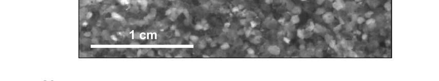
20 Abstract, Fall Meeting of the American Geophysical Union, San Francisco. Ganti, V., M. M. Meerschaert, E. Foufoula-Georgiou, E. Viparelli, and G. Parker (2010), Normal and anomalous diffusion of gravel tracer particles in rivers, Journal of Geophysical Research Earth Surface, 115, F00A12, doi: /2008JF Gibbs, J. W. (1902), Elementary Principles in Statistical Mechanics, New Haven, Yale University Press. Hassan, M. A., and M. Church (1991), Distance of movement of coarse particles in gravel bed streams, Water Resources Research, 27, Hill, K. M., L. DellAngelo, and M. M. Meerschaert (2010), Heavy-tailed travel distance in gravel bed transport: An exploratory enquiry, Journal of Geophysical Research Earth Surface, 115, F00A14, doi: /2009JF Lajeunesse, E., L. Malverti, and F. Charru (2010), Bed load transport in turbulent flow at the grain scale: Experiments and modeling, Journal of Geophysical Research Earth Surface, 115, F04001, doi: /2009JF Lisle, I. G., C. W. Rose, W. L. Hogarth, P. B. Hairsine, G. C. Sander, and J. Y. Parkange (1998), Stochastic sediment transport in soil erosion, Journal of Hydrology, 204, Martin, R. L., D. J. Jerolmack, and R. Schumer (2012), The physical basis for anomalous diffusion in bedload transport, Journal of Geophysical Research Earth Surface, doi: /2011JF (in press) McLean, S. R., J. M. Nelson, and S. R. Wolfe (1994), Turbulence structure over two-dimensional bed forms: Implication for sediment transport, Journal of Geophysical Research, 99, Metzler, R., and J. Klafter (2000), The random walk s guide to anomalous diffusion: a fractional dynamics approach, Physics Reports, 339, Nelson, J. M., R. L. Shreve, S. R. McLean, and T. G. Drake (1995), Role of near-bed turbulence structure in bed load transport and bed form mechanics, Water Resources Research, 31, Nikora, V., H. Habersack, T. Huber, and I. McEwan (2002), On bed particle diffusion in gravel bed flows under weak bed load transport, Water Resources Research, 38, 1081, doi: /2001WR Reynolds, A. M., A. D. Smith, R. Menzel, U, Greggers, D. R. Reynolds, and J. R. Riley (2007), Displaced honey bees perform optimal scale-free search flights, Ecology, 88, Sayre, W., and D. Hubbell (1965), Transport and dispersion of labeled bed material, North Loup River, Nebraska, U.S. Geological Survey Professional Paper, 433-C, 48 pp. Schmeeckle, M. W., and D. J. Furbish (2007), A Fokker-Planck model of bedload transport and morphodynamics, Abstract presented at the Stochastic Transport and Emerging Scaling on Earth s Surface (STRESS) work group meeting, Lake Tahoe, Nevada, sponsored by National Center for Earth-surface Dynamics, the University of Illinois, and the Desert Research Institute. Schmeeckle, M. W., and J. M. Nelson (2003), Direct numerical simulation of bedload transport using a local, dynamic boundary condition, Sedimentology, 50, Schumer, R., M. M. Meerschaert, and B. Baeumer (2009), Fractional advection-dispersion equations for modeling transport at the Earth surface, Journal of Geophysical Research Earth Surface, 114, F00A07, doi: /2008JF Singh, A., K. Fienberg, D. J. Jerolmack, J. Marr, and E. Foufoula-Georgiou (2009), Experimental evidence for statistical scaling and intermittency in sediment transport rates, Journal of Geophysical Research Earth Surface, 114, F01025, doi: /2007JF Taylor, G. I. (1921), Diffusion by continuous movements, Proceedings of the London Mathematical Society, 20, Viswanathan, G. M., E. P. Raposo, F. Bartumeus, J. Catalan, and M. G. E. Da Luz (2005), Necessary criterion for distinguishing true superdiffusion from correlated random walk processes, Physical Review E, 72, , doi: /PhysRevE D. J. Furbish, Department of Earth and Environmental Sciences, Vanderbilt University, 2301 Vanderbilt Place, Station B 35805, Nashville, Tennessee 37235, USA. (david.j.furbish@vanderbilt.edu) J. C. Roseberry, Department of Earth and Environmental Sciences, Vanderbilt University, 2301 Vanderbilt Place, Station B 35805, Nashville, Tennessee 37235, USA. (john.c.roseberry@vanderbilt.edu) M. W. Schmeeckle, School of Geographical Sciences, Arizona State University, Tempe, Arizona 85287, USA. (schmeeckle@asu.edu) Figure Captions Figure 1. Pixelated image of sediment bed showing procedure for tracking streamwise and crossstream displacements of particles between successive frames for runs R2B and R3B. Figure 2. Map view of R3B sampling area B showing partitions db and particle motions occurring during the 0.4 sec time series; note that some particles start to move early in the series (green) 20

21 and some start late (red), where clustering of motions partly reflects effects of turbulent sweeps. Figure 3. Time series plots of particle activity n(t; db) for R2B and R3B; partitions db coincide with those shown in Figure 2. Figure 4. Plot of coefficient of variation C n of particle activity versus partition area db for R1 (open circle), R2 and R2B (black circles), R3 and R3B (black triangles), and R5 (open triangle); points for R2B and R3B at db = 5.7 cm, 11.4 cm and 22.9 cm are averages of partitions shown in /2 Figure 2 and Figure 3; dashed lines coincide with C n ~ db. Figure 5. Examples of the autocorrelation function r n(k) of the particle activity n for R1, R2, R2B and R3B. Figure 6. Plots of observed (histograms) versus theoretical (points) probability distributions P n(n db) of the number of particles n db within the sampling area db for (a) R1, (b) R2, (c) R3 and (d) R5, with estimated fifth and ninety-fifth percentiles (bars) about the expected values. Figure 7. Proportions of particle velocities measured at sec and sec following entrainment, and at sec and sec preceding deposition; data from R3B. Figure 8. Example from R3B of particle motion in plan view, with time series of streamwise velocity u p and cross-stream velocity v p. Figure 9. Discrete probability density of streamwise velocities u p, and semi-log plot (inset) of probability density versus u p with straight-line fit to data (R2) illustrating exponential-like form of distribution; data for R1, R3, R5, R2B and R3B all show this exponential-like form. Figure 10. Discrete probability density of cross-stream velocities v p, and semi-log plot (inset) of probability density versus vp with straight-line fit to data (R2) illustrating exponential-like form of one-sided distribution; data for R1, R3, R5, R2B and R3B all show this exponential-like form. Figure 11. Example (R3B) time series of average streamwise velocity u and average cross-stream velocity v; note that u fluctuates about the average u = = 4.6 cm s whereas v exhibits drift over the short time series (0.4 sec). Figure 12. Autocorrelation function r u(k) of average streamwise velocity u from Figure 12. Figure 13. Plot of particle hop distance versus travel time for R2B (open circles) and R3B 5/3 (closed circles), showing ~ relation (inset); points significantly below ~ 0.01 are effectively zero, representing measurement error. Figure 14. Observed (histograms) and fitted (lines) gamma distributions of particle hop distance and travel time ; data from R3B. Figure 15. Examples (gray and black circles) of mean squared displacements R(k) versus time interval k for individual particles from R2B exhibiting periodic structure of motions and apparent superdiffusive behavior ( > 1), and (open circles) R(k) calculated for all particle motions. Figure 16. Examples of mean squared displacement R(k) versus time interval k for pooled particle motions from R1 (black), R2 (gray) and R3 (clear) showing ballistic behavior ( ~ 2) at small k and apparent superdiffusive behavior ( > 1) with increasing k. Figure 17. Plots of disentrainment functions P ( ) and P ( ) (solid lines), based on fits to gamma distributions f ( ) and f ( ) (dashed lines) in Figure 14. Figure 18. Plots of (a) particle activity n (circles) and average streamwise particle velocity (triangles) versus dimensionless bed stress * for R1, R2, R3, R5 (black symbols) and R2B, R3B 1/2 (gray symbols), where line through velocity data coincides with ~ ; and (b) dimensionless flux q * versus dimensionless shear stress * showing experimental values (circles) and transport relation (line) provided by Lajeunesse et al. [2010] assuming a dimensionless critical stress ~ * 21

22 0.04. Figure A1. Example of position versus time for particles from R2B, and relative displacement about mean trajectory, showing that motion is dominated by a fundamental harmonic with period or 2 ; most particles display one of these harmonics, and a few display dominant higher harmonics (e.g. with period /2); these harmonics are present in motions involving both short and long travel times. Figure A2. Plot of mean squared displacement R(k) versus time interval k for the two particles in Figure A1; solid lines are equation (A4), dashed lines are equation (A5), and points are values of R(k) calculated for (solid circles) hop distance = 1.59 cm, period = sec, and estimated amplitude a = cm, and (open circles) = 0.35 cm, period 2 = sec, and a = 0.12 cm. Figure A3. Plot of mean squared displacement R(k) versus time interval k calculated for motions of a group of particles, each involving (closed circles) a correlated random walk consisting of the sum of uncorrelated Brownian-like motions and a small-amplitude sinusoid, where the amplitude, period and phase of each sinusoid are randomly selected, and (open circles) Brownian-like motions without sinusoidal parts. Table 1. Experimental Conditions. Run Sampling window size (pixels) Run time (sec) Sampling interval (sec) Mean activity -2 (number cm ) Mean particle velocity (cm s ) R R R R R2B R3B

23 Figure 1

24 Figure 2

25 Figure 3

26 Figure 4

27 Figure 5

28 Figure 6

29 0.4 1 Frame Before Entrainment 5 Frames Before Entrainment 0.3 Proportion Frame Before Deposition 5 Frames Before Deposition Proportion Figure 7 Streamwise velocity u p (cm s )

30 Figure 8