Deterministic Scheduling. Dr inż. Krzysztof Giaro Gdańsk University of Technology
|
|
|
- Lillian Dawson
- 6 years ago
- Views:
Transcription

1 Deterministic Scheduling Dr inż. Krzysztof Giaro Gdańsk University of Technology
2 Lecture Plan Introduction to deterministic scheduling Critical path metod Some discrete optimization problems Scheduling to minimize C max Scheduling to minimize ΣC i Scheduling to minimize L max Scheduling to minimize number of tardy tasks Scheduling on dedicated processors
3 Introduction to Deterministic Scheduling Our aim is to schedule the given set of tasks (programs etc.) on machines (or processors). We have to construct a schedule that fulfils given constraints and minimizes optimality criterion (objective function). Deterministic model: all the parameters of the system and of the tasks are known in advance. Genesis and practical motivations: scheduling manufacturing processes, project planning, school or conference timetabling, scheduling tasks in multitask operating systems, distributed computing.
4 Introduction to Deterministic Scheduling Example 1. Five tasks with processing times p 1,...,p 5 =6,9,4,1,4 have to be scheduled on three processors to minimize schedule length. M 1 J 2 M 2 J 1 J 4 M 3 J 3 J 5 Graphical representation of a schedule - Gantt chart 9 Why the above schedule is feasible? General constriants in classical scheduling theory: each task is processed by at most one processor at a time, each processor is capable of processing at most one task at a time, other constraints - to be discussed...
5 Introduction to Deterministic Scheduling Processors characterization Parallel processors (each processor is capable to process each task): identical processors every processor is of the same speed, uniform processors processors differ in speed, but the speed does not depend on the task, unrelated processors the speed of the processor depend on the particular task processed. M 1 J 2 M 2 J 1 J 4 M 3 J 3 J 5 Schedule on three parallel processors 9
6 Introduction to Deterministic Scheduling Processors characterization Dedicated processors Each job consists of the set of tasks preassigned to processors (job J j consists of tasks T ij preassigned to M i, of processing time p ij ). The job is completed at the time the latest task is completed, some jobs may not need all the processors (empty operations), no two tasks of the same job can be scheduled in parallel, a processor is capable to process at most one task at a time. There are three models of scheduling on dedicated processors: flow shop all jobs have the same processing order through the machines coincident with machine numbering, open shop the sequenice of tasks within each job is arbitrary, job shop the machine sequence of each job is given and may differ between jobs.
7 Introduction to Deterministic Scheduling Processors characterization Dedicated processors - open shop (processor sequence is arbitrary for each job). Example. One day school timetable. Teachers M 1 J 2 J 1 J 3 Classes M 1 M 2 M 3 J J J M 2 M 3 J Z J J 3 J 1 J 3 J 2 7
8 Introduction to Deterministic Scheduling Processors characterization Dedicated processors - flow shop (processor sequence is the same for each job - task T ij must precede T kj for i<k). Example. Conveyor belt. J a J b J c Details M 1 M 2 M 3 Robots M 1 M 2 M 3 J J J M 1 M 2 M 3 J 1 J 3 J 2 J 3 J 1 Z 1 J 2 J 1 J 3 J 2 10
9 Introduction to Deterministic Scheduling Processors characterization Dedicated processors - flow shop (processor sequence is the same for each job - task T ij must precede T kj for i<k). Flow shop allow the job order to differ between machines... M 1 M 2 J 1 J 3 J 2 J 3 J 1 Z 1 J 2 M 3 J 3 J 1 J 2 10 M 1 J 1 J 3 J 2 M 2 J 3 J 1 Z 1 J 2 Permutation flow shop does not. M 3 J 1 J 3 J 2 10 Dedicated processors will be considered later...
10 Introduction to Deterministic Scheduling Tasks characterization There are given: the set of n tasks T={T 1,...,T n } and m machines (processors) M={M 1,...,M m }. Task T j : Processing time. It is independent of processor in case of identical processors and is denoted p j. In the case of uniform processors, processor M i speed is denoted b i, and the processing time of T j on M i is p j /b i. In the case of unrelated processors the processing time of T j on M i is p ij. Release (or arrival) time r j. The time at which the task is ready for processing. By default all release times are zero. Due date d j. Specifies the time limit by which should be completed. Usually, penalty functions are defined in accordance with due dates, or d j denotes the hard time limit (deadline) by which T j must be completed (exact meaning comes from the context). Weight w j expresses the relative urgency of T j, by default w j =1.
11 Introduction to Deterministic Scheduling Tasks characterization Dependent tasks: In the task set there are some precedence constraints defined by a precedence relation. T i pt j means that task T j cannot be started until T i is completed (e.g. T j needs the results of T i ). In the case there are no precedence constraints, we say that the tasks are independent (by default). In the other case we say the tasks are dependent. The precedence relation is usually represented as a directed graph in shich nodes correspond to tasks and arcs represent precedence constraints (task-on-node graph). Transitive arcs are usually removed from precedence graph.
12 Introduction to Deterministic Scheduling Tasks characterization Example. A schedule for 10 dependent tasks (p j given in the nodes). T 1 2 T 2 3 T 3 1 T 4 2 T 6 T T 8 T 7 2 M 1 T 1 T 3 T 10 T 5 T 10 1 M 2 T 2 T 6 T 8 M 3 T 3 T 4 Z 1 T 7 Z 1 T 9 T
13 Introduction to Deterministic Scheduling Tasks characterization A schedule can be: non-preemptive preempting of any task is not allowed (default), preemptive each task may be preempted at any time and restarted later (even on a different processor) with no cost. M 1 T 2 M 2 T 1 T 3 T 1 M 3 T 3 T 3 Preemptive schedule on parallel processors 9
14 Introduction to Deterministic Scheduling Feasible schedule conditions (gathered): each processor is assigned to at most one task at a time, each task is processed by at most one machine at a time, task T j is processed completly in the time interval [r j, ) (or within [r j, d j ), when deadlines are present), precedence constraints are satisfied, in the case of non-preemptive scheduling no task is preempted, otherwise the number of preemptions is finite.
15 Introduction to Deterministic Scheduling Optimization criteria A location of the task T i within the schedule: completion time C i, flow time F i = C i r i, lateness L i = C i d i, tardiness T i = max{c i d i,0}, tardiness flag U i = w(c i >d i ), i.e. the answer (0/1 logical yes/no) to the question whether the task is late or not.
16 Introduction to Deterministic Scheduling Optimization criteria Most common optimization criteria: schedule length (makespan) C max = max{c j : j=1,...,n}, sum of completion times (total completion time) ΣC j = Σ i=1,...,n C i, mean flow time F = (Σ i=1,...,n F i )/n. M 1 M 2 M 3 Z 3 Z 1 Z 2 Z 5 Z 4 C max = 9, ΣC j = = 34 A schedule of three parallel processors. p 1,...,p 5 =6,9,4,1,4. 9 In the case there are tasks weights we can consider: sum of weighted completion times Σw j C j = Σ i=1,...,n w i C i, w 1,...,w 5 =1,2,3,1,1 Σw j C j = = 51
17 Introduction to Deterministic Scheduling Optimization criteria Related to due times: maximum lateness L max = max{l j : j=1,...,n}, maximum tardiness T max = max{t j : j=1,...,n}, total tardiness ΣT j = Σ i=1,...,n T i, number of tardy tasks ΣU j = Σ i=1,...,n U i, weighted criteria may be considered, e.g. total weighted tardiness Σw j T j = Σ i=1,...,n w i T i. M 1 M 2 M 3 T 1 T 2 T 4 Task: T 1 T 2 T 3 T 4 T 5 d i = L i = T i = T 3 T 5 L = T max max = 2 Some criteria are pair-wise equivalent ΣL i = ΣC i Σd i, F= (ΣC i )/n (Σr i )/n. 9 ΣT j = 4, ΣU j = 2
18 Introduction to Deterministic Scheduling Classification of deterministic scheduling problems. α β γ Procession environment Task characteristics Optimization criterion α is of the form: P identical processors Q uniform processors R unrelated processors O open shop F flow shop PF permutation flow shop J job shop Moreover: there may be specified the number of processors e.g. O4, in the case of single processors we just put 1, we put in the case of processorfree environment.
19 Introduction to Deterministic Scheduling Classification of deterministic scheduling problems. In the case β is empty all tasks characteristics are default: the tasks are non-preemptive, not dependent r j =0, processing times and due dates are arbitrary. β possible values: pmtn preemptive tasks, res additional resources required (omitted), prec there are precedence constraints, r j arrival times differ per task, p j =1 or UET all processing times equal to 1 unit, p ij {0,1} or ZUET all tasks are of unit time or empty (dedicated processors), C j d j or d j denote deadlines,
20 Introduction to Deterministic Scheduling Classification of deterministic scheduling problems. β possible values: in tree, out tree, chains... reflects the precedence constraints (prec). in tree out tree
21 Introduction to Deterministic Scheduling Classification of deterministic scheduling problems. Examples. P3 prec C max scheduling non-preemptive tasks with precedence constraints on three parallel identical processors to minimize schedule length. R pmtn,prec,r i ΣU i scheduling preemptive dependent tasks with arbitrary ready times and arbitrary due dates on parallel unrelated processors to minimize the number ot tardy tasks. 1 r i,c i d i decision problem of existence (no optimization criterion) of schedule of independent tasks with arbitrary ready times and deadlines on a single processor, such that no task is tardy.
22 Introduction to Deterministic Scheduling Propertiels of computer algorithm evaluating its quality. Computational (time) complexity function that estimates (upper bound) the worst-case operation number performed during execution in terms of input data size. Polynomial (time) algorithm when time complexity may be bounded by some polynomial of data size. In computing theory polynomial algorithms are considered as efficient.
23 Introduction to Deterministic Scheduling Propertiels of computer algorithm evaluating its quality. NP-hard problems are commonly believed not to have polynomial time algorithms solving them. For these problems we can only use fast but not accurate procedures or (for small instances) long time heuristics. NP-hardness is treated as computational intractability. How to prove that problem A is NP-hard? Sketch: Find any NP-hard problem B and show the efficient (polynomial) procedure that reduces (translates) B into A. Then A is not less general problem than B, therefore if B was hard, so is A.
24 Introduction to Deterministic Scheduling Reductions of scheduling problems R w i F i w i T i w i U i Q Rm p i =1 P Qm prec F T i U i Pm in-tree out-tree L max r j 1 chain C max
25 Introduction to Deterministic Scheduling Computational complexity of scheduling problems In we restrict the number of processors to 1,2,3,, there are 4536 problems: 416 polynomial-time solvable, 3817 NP hard, 303 open. How do we cope with NP-hardness? exact pseudo-polynomial time algorithms, exact algorithms, efficient only in the mean-case, heuristics (tabu-search, genetic algorithms etc.), in the case of small input data - exponential exchaustive search (e.g. branch bound).
26 Introduction to Deterministic Scheduling General problem analysis schema Optimization problem X decision version X d Construct effective algorithm solving X Construct pseudopolynomial time algorithm for X X d P? X d NPC? X d PseudoP? X d NPC!? Polynomial-time: approximate algorithms approximation schemas Do not exist Yes Small data: exhaistive search (branch & bound) Heuristicss: tabu search, genetic algorithms,... Do approximations satisfy us? No Restrict problem X
27 Critical path method. prec C max model consists of a set of dependent tasks of arbitrary lengths, which do not need processors. Our aim is to construct a schedule of minimum length. Precedence relation p is a quasi order in the set of tasks, i.e. it is: anti-reflective: transistive: T Ti p T i ( i ) T, T, T Ti p Tj Tj p Tk Ti p Tk i j k
28 Critical path method. Precence relation p is represented with an acyclic digraph. AN (activity on node) network: nodes correspond to tasks, nodes weights equal to processing times, T i pt j there exists a directed path connecting node T i and node T j, transitive arcs are removed. AA (activity on arc) network: arcs correspond to tasks, their length is equal to processing times, for each node v there exists a path starting at S (source) and terminating at T (sink) passing through v, T i pt j arc T i end-node is the starting-node of T j, or there exists a directed path starting at T i end-node and terminating at T j start-node., to construct the network one may need to add apparent tasks zero-length tasks.
29 Critical path method. Example. Precedence relation for 19 tasks. Z 1,3 Z 4,2 Z 8,2 Z 13,6 Z 5,4 Z 9,1 Z 14,5 Z 2,8 Z 3,2 Z 6,6 Z 7,9 Z 10,2 Z 11,1 Z 12,2 Z 15,9 Z 16,6 Z 17,2 AN network Z 18,5 Z 19,3 AA network A Z D F I 4,2 Z 8,2 Z 13,6 Z 1,3 Z 5,4 Z 9,1 Z 14,5 Z 18,5 C G Z Z 2,8 Z 10,2 Z 15,9 U Z 3,2 Z 6,6 Z 11,1 Z 16,6 Z 19,3 B Z 7,9 E Z 12,2 H Z 17,2 J Example. Translating AN to AA we may need to add (zero-length) apparent tasks. T 1 T 3 S T 1 A T 3 T 0 p 0 =0 T T 2 T 4 T 2 B T 4
30 Critical path method. prec C max model consists of a set of dependent tasks of arbitrary lengths, which do not need processors. Our aim is to construct a schedule of minimum length. The idea: for every task T i we find the earliest possible start time l(t i ), i.e. the length of the longest path terminating at that task. How to find these start times? AN network Algorithm: 1. find a topological node ordering (the start of any arc precedes its end), 2. assign l(t a )=0 for every task T a without predecessor, 3. assing l(t a )=max{l(t j )+p j : exists an arc(t j, T i )} to all other tasks in topological order. AA network Algorithm: 1. find a topological node ordering, 2. l(s)=0, assign l(v)=max{l(u)+p j : arc T j connects u and v} to each node v, Result: l(t j ) is equal to l(v) of the starting node v of T j. l(t) is the length of an optimal schedule.
31 Critical path method. Example: construction of a schedule for 19 tasks. A T D F T I 4,2 T 8,2 13,6 T 1,3 T 5,4 T 9,1 T 14,5 T 18,5 T C G S 2,8 T 10,2 T 15,9 T T 3,2 T 6,6 T 11,1 T 16,6 T 19,3 B T 7,9 E T 12,2 H T 17,2 J Topological order S: A: B: C: D: E: F: G: H: I: J: T: Starting Z:0+3 times Z:0+2 Z:0+8, A:3+4, B:2+6 A:3+2 B:2+9 C:8+1,D:5+2 C:8+2, E:11+1 E:11+2 F:9+6, G:12+5 G:12+6, H:13+2 I:17+5, J:18+3, G:12+9
32 S: A: B: C: D: E: F: G: H: I: J: T: A T 4,2 Critical path method. D T 8,2 F T I 13,6 T 1,3 T 1,3 T 5,4 T 9,1 T 14,5 T 18,5 T 3,2 T S 2,8 C Z G 10,2 T 15,9 T 0 3 T 3,2 2 T 6,6 T 11,1 T 16,6 T 19,3 8 5 B T 7,9 E T 12,2 H T 17,2 J 11 T 7 9 T T 3 T 5 T T 2 T T 1 T 4 T 8 T 9 T 12 T 11 T 4,2 T 5,4 T 2,8 T 6,6 T 7, T 16 T 15 T 17 T 14 T 8,2 T 9,1 T 10,2 T 11,1 T 12,2 T 13,6 T 14,5 T 15,9 T 16, 6 T 17,2 T 18 T 19 T 18,5 T 19,3
33 Critical path method. Critical path method does not only minimize C max, but also optimizes all previously defined criteria. We can introduce to the model arbitrary release times by adding for each task T j extra task of length r j preceding T j.
34 Some Discrete Optimization Problems maximum flow problem. There is given a loop-free multidigraph D(V,E) where each arc is assigned a capacity w:e N. There are two specified nodes - the source s and the sink t. The aim is to find a flow f:e N {0} of maximum value. What is a flow of value F? e E f(e) c(e), (flows may not exceed capacities) v V {z,u} Σ e terminates at v f(e) Σ e starts at v f(e) = 0, (the same flows in and flows out for every ordinary node) Σ e terminates at t f(e) Σ e starts at t f(e) = F, (F units flow out of the network through the sink) Σ e terminates at s f(e) Σ e starts at s f(e) = F. (F units flow into the network through the source)
35 Some Discrete Optimization Problems maximum flow problem. There is given a loop-free multidigraph D(V,E) where each arc is assigned a capacity w:e N. There are two specified nodes - the source s and the sink t. The aim is to find a flow f:e N {0} of maximum value S T Network, arcs capacity
36 Some Discrete Optimization Problems maximum flow problem. There is given a loop-free multidigraph D(V,E) where each arc is assigned a capacity w:e N. There are two specified nodes - the source s and the sink t. The aim is to find a flow f:e N {0} of maximum value. 5/2 2/2 1/0 1/0 3/2 S 2/2 3/1 2/2 2/1 1/1 1/1 4/1 T... and maximum flow F=5 Complexity O( V E log( V 2 E ) O( V 3 ).
37 Some Discrete Optimization Problems Many graph coloring models. Longest (shortest) path problems. Linear programming polynomial-time algorithm known. The problem of graph matching. There is given graph G(V,E) with a weight function w:e N {0}. A matching is a subset A E of pair-wise non-neighbouring edges. Maximum matching: find a matching of the maximum possible cardinality (α(l(g))). The complexity O( E V 1/2 ). Heaviest (lightest) matching of a given cardinality. For a given k α(l(g)) find a matching of cardinality k and maximum (minmum) possible weight sum. Heaviest matching. Find a matching of maximum possible weight sum. The complexity O( V 3 ) for bipartite graphs and O( V 4 ) in general case.
38 Some Discrete Optimization Problems Cardinality: 4 Weight: 4 1 Cardinality: 3 Weight: 12 Maximum matching needs not to be the heaviest one and vice-versa.
39 Scheduling on Parallel Processors to Minimize the Schedule Length. Identical processors, independent tasks Preemptive scheduling P pmtn C max. McNaughton Algorithm (complexity O(n)) 1. Derive optimal length C max *=max{σ j=1,...,n p j /m, max j=1,...,n p j }, 2. Schedule the consecutive tasks on the first machine until C max * is reached. Then interrupt the processed task (if it is not completed) and continue processing it on the next machine starting at the moment 0. Example. m=3, n=5, p 1,...,p 5 =4,5,2,1,2. Σ i=1,...,5 p i =14, max p i =5, C max *=max{14/3,5}=5. M 1 T Z 1 TZ 2 M 2 TZ 2 TZ 3 M 3 TZ 3 TZ 4 T 5 5
40 Scheduling on Parallel Processors to Minimize the Schedule Length. Identical processors, independent tasks Non-preemptive scheduling P C max. The problem is NP-hard even in the case of two processors (P2 C max ). Proof. Partition Problem: there is given a sequence of positive integers a 1,...a n such that S=Σ i=1,...,n a i. Determine if there exists a sub-sequence of sum S/2? PP P2 C max reduction: put n tasks of lengths p j =a j (j=1,...,n), and two processors. Determine if C max S/2. M 1 p i... M 2... There exists an exact pseudo-polynomial dynamic programming algorithm of complexity O(nC m ), for some C C max *. S/2
41 Scheduling on Parallel Processors to Minimize the Schedule Length. Identical processors, independent tasks Non-preemptive scheduling P C max. Polynomial-time approximation algorithms. List Scheduling LS - an algorithm used in numerous problems: fix an ordering of the tasks on the list, any time a processor gets free (a task processed by that processor has been completed), schedule the first available task from the list on that processor. Example. m=3, n=5, p 1,...,p 5 =2,2,1,1,3. M 1 T 1 T 5 M 1 T 5 M 2 T 2 M 2 T 1 T 3 M 3 T 3 T 4 M 3 T 2 T 4 5 List scheduling Optimal scheduling 3
42 Scheduling on Parallel Processors to Minimize the Schedule Length. Identical processors, independent tasks Non-preemptive scheduling P C max. Polynomial-time approximation algorithms. List Scheduling LS - an algorithm used in numerous problems: fix an ordering of the tasks on the list, any time a processor gets free (a task processed by that processor has been completed), schedule the first available task from the list on that processor. Approximation ratio. LS is 2 approximate: C max (LS) (2 m 1 )C max *. Proof (includes dependent tasks model P prec C max ). Consider a sequence of tasks T π(1),... T π(k) in a LS schedule, such that T π(1) - the last completed task, T π(2) - the last completed predecessor of T π(1) etc. C max (pmtn) C max * C max (LS) i=1,...,k p π(k) + i π p i /m =(1 1/m) i=1,...,k p π(k) + i p i /m (2 m 1 ) C max (pmtn) (2 m 1 ) C max *
43 Scheduling on Parallel Processors to Minimize the Schedule Length. Identical processors, independent tasks Non-preemptive scheduling P C max. Polynomial-time approximation algorithms. Approximation ratio. LS is 2 approximate: C max (LS) (2 m 1 )C max *. Proof C (pmtn) max C max * (preemptions may help) C max * C max (LS) (optimal vs non-optimal) C max (LS) i=1,...,k p π(k) + i π p i /m (p π(1) is the last completed job) i=1,...,k p π(k) + i π p i /m=(1 1/m) i=1,...,k p π(k) + i p i /m (1 1/m) i=1,...,k p π(k) + i p i /m (2 m 1 ) C max (pmtn) because (1 m 1 ) i=1,...,k p π(k) (1 m 1 ) C max (pmtn) (prec. constraints) (2 m 1 ) C max (pmtn) (2 m 1 ) C max * (see first step)
44 Scheduling on Parallel Processors to Minimize the Schedule Length. Identical processors, independent tasks Non-preemptive scheuling P C max. Polynomial-time approximation algorithms. LPT (Longest Processing Time) scheduling: List scheduling, where the tasks are sorted in non-increasing processing times p i order. Approximation ratio.ls is 4/3 approximate: C max (LPT) (4/3 (3m) 1 )C max *. Unrelated processors, not dependent tasks Preemptive scheduling R pmtn C max Polynomial time algorithm - to be discussed later... Non-preemptive scheduling R C max The problem is NP hard (generalization of P C max ). Subproblem Q p i =1 C max is solvable in polynomial time. LPT is used in practice.
45 Scheduling on Parallel Processors to Minimize the Schedule Length. Identical processors, dependent tasks Preemptive scheduling P pmtn,prec C max. The problem is NP hard. P2 pmtn,prec C max i P pmtn,forest C max are solvable in O(n 2 ) time. The following inequality estimating preemptive, non-preemptive and LS schedule holds: C* max (2 m 1 )C* max (pmtn) Proof. The same as in the case of not dependent tasks.
46 Scheduling on Parallel Processors to Minimize the Schedule Length. Identical processors, dependent tasks Non-preemptive scheduling P prec C max. Obviously the problem is NP-hard. Many unit-time processing time cases are known to be solvable in polynomial time: P p i =1,in forest C max and P p i =1,out forest C max (Hu algorithm, complexity O(n)), P2 p i =1,prec C max (Coffman-Graham algorithm, complexity O(n 2 )), Even P p i =1,opositing forest C max and P p i ={1,2},prec C max is NP hard. Hu algorithm: out forest in forest reduction: reverse the precedence relation. Solve the problem and reverse the obtained schedule. in forest in tree: add extra task dependent of all the roots. After obtaining the solution, remove this task from the schedule. Hu algorithm sketch: list scheduling for dependent tasks + descending distance from the root order.
47 Scheduling on Parallel Processors to Minimize the Schedule Length. Identical processors, dependent tasks Non-preemptive scheduling Hu algorithm (P p i =1,in tree C max ): Level of a task number of nodes in the path to the root. The task is avaliable at the moment t if all the tasks dependent of that task have been completed until t. Compute the levels of the tasks; t:=1; repeat Find the list L t of all tasks avalable at the moment t; Sort L t in non-increasing levels order; Assign m (or less) forst tasks from L t to the processors; Remove the scheduled tasks from the graph; t:=t+1; until all the tasks are scheduled;
48 Scheduling on Parallel Processors to Minimize the Schedule Length. Identical processors, dependent tasks Non-preemptive scheduling Example. Hu algorithm. n=12, m=3. 4 T 1 T 2 T 3 T 4 T 5 - avalable tasks 3 T 6 T 7 T 8 T 9 2 T 10 T 11 1 T 12
49 Scheduling on Parallel Processors to Minimize the Schedule Length. Identical processors, dependent tasks Non-preemptive scheduling Example. Hu algorithm. n=12, m=3. 4 T 1 T 2 T 3 T 4 T 5 3 T 6 T 7 T 8 T 9 2 T 10 T 11 M 1 M 2 1 T 12 M 3 5
50 Scheduling on Parallel Processors to Minimize the Schedule Length. Identical processors, dependent tasks Non-preemptive scheduling Example. Hu algorithm. n=12, m=3. 4 T 1 T 2 T 3 T 4 T 5 3 T 6 T 7 T 8 T 9 2 T 10 T 11 M 1 T 1 M 2 T 2 1 T 12 M 3 T 3 5
51 Scheduling on Parallel Processors to Minimize the Schedule Length. Identical processors, dependent tasks Non-preemptive scheduling Example. Hu algorithm. n=12, m=3. 4 T 1 T 2 T 3 T 4 T 5 3 T 6 T 7 T 8 T 9 2 T 10 T 11 M 1 T 1 T 4 M 2 T 2 T 5 1 T 12 M 3 T 3 T 6 5
52 Scheduling on Parallel Processors to Minimize the Schedule Length. Identical processors, dependent tasks Non-preemptive scheduling Example. Hu algorithm. n=12, m=3. 4 T 1 T 2 T 3 T 4 T 5 3 T 6 T 7 T 8 T 9 2 T 10 T 11 M 1 T 1 T 4 T 7 M 2 T 2 T 5 T 8 1 T 12 M 3 T 3 T 6 T 9 5
53 Scheduling on Parallel Processors to Minimize the Schedule Length. Identical processors, dependent tasks Non-preemptive scheduling Example. Hu algorithm. n=12, m=3. 4 T 1 T 2 T 3 T 4 T 5 3 T 6 T 7 T 8 T 9 2 T 10 T 11 M 1 TZ 1 TZ 4 TZ 7 TZ 10 T 12 M 2 TZ 2 TZ 5 TZ 8 TZ 11 1 T 12 M 3 TZ 3 TZ 6 TZ 9 5
54 Scheduling on Parallel Processors to Minimize the Schedule Length. Identical processors, dependent tasks Non-preemptive scheduling Coffman-Graham algorithm (P2 prec C max ): 1. label the tasks with integers l from range [1,..., n] 2. list scheduling, with desscening labels order. Phase 1 - task labeling; no task has any label or list at the beginning; for i:=1 to n do begin A:=the set of tasks without label, for which all dependent tasks are labeled; for each T A do assign the descending sequence of the labels of tasks dependent of T to list(t); choose T A with the lexicographic minimum list(t); l(t):=i; end;

55 Scheduling on Parallel Processors to Minimize the Schedule Length. Identical processors, dependent tasks Non-preemptive scheduling Example. Coffman-Graham algorithm, n = 17

56 Scheduling on Parallel Processors to Minimize the Schedule Length. Identical processors, dependent tasks Non-preemptive scheduling Example. Coffman-Graham algorithm, n = 17
57 Scheduling on Parallel Processors to Minimize the Schedule Length. Identical processors, dependent tasks Non-preemptive scheduling LS heuristic can be applied to P prec C max. The solution is 2- approximate: C* max (LS) (2 m 1 )C* max Proof: It has been proved already... The order on the list (priority) can be chosen in many different ways. However, some anomalies may occur, i.e. the schedule may lenghten while: increasing the number of processors, decreasing the processing times, releasing some precedence constraints, changing the list order.
58 Scheduling on Parallel Processors to Minimize the Mean Flow Time Identical processors, independent tasks Proposal: task Z j scheduled in the k-th position on machine M i increments the value of ΣC j by kp j (or kp ij in the case of R...). M Z a Z b Z c Corollaries. the processing time of the first task is multiplied by the greatest coefficient; the coefficients of the following tasks are decreasing, to minimize ΣC j we should schedule short tasks first (as they are multiplied by the greatest coefficients), list scheduling with the SPT rule (Shortest Processing Times) leads to an optimal solution on a single processor, how to assign the tasks to the processors?
59 Scheduling on Parallel Processors to Minimize the Mean Flow Time Identical processors, independent tasks Both preemptive and non-preemptive cases The problems P ΣC i and P pmtn ΣC i can be considered together (preemptions do not improve the criterion). Optimal algorithm O(nlog n): 1. Suppose the number of tasks is a multiplicity of m (introduce empty tasks if needed), 2. Sort the tasks according to SPT, 3. Assing the following m tuples of tasks to the processors arbitrarily. Example. m=2, n=5, p 1,...,p 5 =2,5,3,1,3. SPT: Z 0 Z 4 Z 1 Z 3 Z 5 Z 2 p i = Empty task M 1 M 2 Z 4 Z 3 Z 1 Z 5 Z 2 ΣC j *=21 8
60 Scheduling on Parallel Processors to Minimize the Mean Flow Time Identical processors, independent tasks Both preemptive and non-preemptive cases The problems P ΣC i and P pmtn ΣC i can be considered together (preemptions do not improve the criterion). Optimal algorithm O(nlog n): 1. Suppose the number of tasks is a multiplicity of m (introduce empty tasks if needed), 2. Sort the tasks according to SPT, 3. Assing the following m tuples of tasks to the processors arbitrarily. Proof (the case of non-preemptive scheduling): Lemma. Suppose a 1,...,a n i b 1,...,b n are sequences of positive integers. How to permutate them in order to make the dot product a π(1) b π(1) +a π(2) b π(2) +...+a π(n-1) b π(n-1) +a π(n) b π(n) the greatest possible? both should be sorted in ascending order, the smallest possible? sort one ascending, the second descending
. Optimal algorithm O(nlog n): 1. Suppose the number of tasks is a multiplicity of m (introduce empty tasks if needed), 2.")
61 Scheduling on Parallel Processors to Minimize the Mean Flow Time Identical processors, independent tasks Both preemptive and non-preemptive cases The problems P ΣC i and P pmtn ΣC i can be considered together (preemptions do not improve the criterion). Optimal algorithm O(nlog n): 1. Suppose the number of tasks is a multiplicity of m (introduce empty tasks if needed), 2. Sort the tasks according to SPT, 3. Assing the following m tuples of tasks to the processors arbitrarily. Proof (the case of non-preemptive scheduling). Consider an optimal scheduling. One may assume that there are k tasks scheduled on each processors (introducing empty tasks if needed). ΣC i = kp π(1) +...+kp π(m) + +(k-1)p π(m+1) +...+(k-1)p π(2m) + +1p π(km-m+1) p π(km) Reordering the tasks according to the SPT rule does not increase ΣC i
62 Scheduling on Parallel Processors to Minimize the Mean Flow Time Identical processors, independent tasks Non-preemptive scheduling In the case the weights are introduced, even P2 Σw j C j is NP-hard. Proof (sketch). Similar to P2 C max. PP P2 Σw i C i reduction: take n tasks with p j = w j =a j (j=1,...,n), two processors. There exists a number C(a 1,...,a n ) such that Σw j C j C(a 1,...,a n ) C max * = Σ i=1,...,n a i /2 (exercise). Following Smith rule in the case of single processor scheduling 1 Σw j C j leads to an optimal solution in O(nlog n) time: sort the tasks in ascending p j /w j order. Proof. Consider the improvement of the criterion caused by changing two consecutive tasks. w j p j + w j (p j +p j ) p i w i w j (p j +p j )= = w i p j p j w i 0 p j /w j p i /w i violating Smith rule increases Σw j C j
63 Scheduling on Parallel Processors to Minimize the Mean Flow Time Non-preemptive scheduling RPT rule can be used in order to minimize both C max and ΣC i : 1. Use the LPT algorithm. 2. Reorder the tasks within each processor due to the SPT rule. Approximation ratio: 1 ΣC i (RPT) /ΣC i * m (commonly better) Identical processors, dependent tasks Even P prec,p j =1 ΣC i, P2 prec,p i {1,2} ΣC i, P2 chains ΣC i and P2 chains,pmtn ΣC i are NP-hard. Polynomial-time algorithms solving P prec,p j =1 ΣC i (Coffman-Graham) and P out-tree,p j =1 ΣC i (adaptation of Hu algorithm) are known. In the case of weighted tasks even single machine scheduling of unit time tasks 1 prec,p j =1 Σw i C i is NP-hard.
64 Scheduling on Parallel Processors to Minimize the Mean Flow Time Unrelated processors, independent tasks O(n 3 ) algorithm for R ΣC i is based on the problem of graph matching. Bipartite weighted graph: Partition V 1 corresponding to the tasks Z 1,...,Z n. Partition V 2 each processor n times: k M i, i=1...m, k=1...n. The edge connecting Z j and k M i is weighted with kp ij (it corresponds to scheduling task Z j on M i, in the k-th position from the end). We construct the lightest matching of n edges, which corresponds to optimal scheduling. Z 1 Z j Z n kp ij 1 M 1 1 M m 2 M 1 km i n M 1 n M m 1 2 k n
65 Scheduling on Parallel Processors to Minimize the Maximum Lateness Properties: L max criterion is a generalization of C max, the problems that are NP hard in the case of minimizing C max remain NP-hard in the case of L max, M Z b Z a M Z a Z b d a d b if we have several tasks of different due times we should start with the most urgent one to minimize maximum lateness, this leads to EDD rule (Earliest Due Date) choose tasks in the ordering of ascending due dates d j, the problem of scheduling on a single processor (1 L max ) is solved by using the EDD rule. d a d b
66 Scheduling on Parallel Processors to Minimize the Maximum Lateness Identical processors, independent tasks Preemptive scheduling Single machine: Liu algorithm O(n 2 ), based on the EDD rule, solves 1 r i,pmtn L max : 1. Choose the task of the smallest due date among available ones, 2. Every time a task has been completed or a new task has arrived go to 1. (in the latter case we preempt currently processed task). Arbitrary number of processors(p r i,pmtn L max ). A polynomial-time algorithm is known: We use sub-routine solving the problem with deadlines P r i,c i d i,pmtn, We find the optimal value of L max using binary search algorithm.
67 Scheduling on Parallel Processors to Minimize the Maximum Lateness P r i,c i d i,pmtn to the problem of maximum flow. First we put the values r i and d i into the ascending sequence e 0 <e 1 <...<e k. We construct a network: The source is connected by k arc of capacity m(e i e i 1 ) to nodes w i, i=1,...,k. The arcs of capacity p i connect nodes-tasks Z i, to the sink; i=1,...,n. We connect w i and Z j by an arc of capacity e i e i 1, iff [e i 1,e i ] [r j,d j ]. Z m(e 1 -e 0 ) m(e i -e i-1 ) m(e k -e k-1 ) w 1 w i e 1 -e 0 e i -e i-1 Z 1 Z j p j p n p 1 U A schedule exists there exists a flow of value Σ i=1,...,n p i (one can distribute the processors among tasks in the time intervals [e i-1, e i ] to complete all the tasks). w k Z n
68 Scheduling on Parallel Processors to Minimize the Maximum Lateness Dependent tasks Non-preemptive scheduling Some NP-hard cases: P2 L max, 1 r j L max. Polynomial-time solvable cases: unit processing times P p j =1,r j L max. similarly for uniform processors Q p j =1 L max (the problem can be reduced to linear programming), single processor scheduling 1 L max solvable using the EDD rule (has been discussed already...).
69 Scheduling on Parallel Processors to Minimize the Maximum Lateness Dependent tasks Preemptive scheduling Single processor scheduling 1 pmtn,prec,r j L max can be solved by a modified Liu algorithm O(n 2 ): 1. Determine modified due dates for each task: d j *=min{d j, min{d i :Z j pz i }} 2. Apply the EDD rule using d j * values, preempting current task in the case a task with smaller modified due-date gets available, 3. Repeat 2 until all the tasks are completed. Some other polynomial-time cases: P pmtn,in tree L max, Q2 pmtn,prec,r j L max. Moreover, some pseudo-polynomial time algorithms are known.
70 Scheduling on Parallel Processors to Minimize the Maximum Lateness Dependent tasks Non-preemptive scheduling Even P p j =1,out tree L max is NP hard. A polynomial-time algorithm for P2 prec,p j =1 L max is known. P p j =1,in tree L max can be solved by Brucker algorithm O(nlog n): next(j) = immediate successor of task T j. 1. Derive modified due dates: d root *=1 d root for the root and d k *=max{1+d next(k) *,1 d k } for other tasks, 2. Schedule the tasks in a similar way as in Hu algorithm, choosing every time the tasks of the largest modified due date instead of the largest distance from the root.
71 Scheduling on Parallel Processors to Minimize the Maximum Lateness Dependent tasks Non-preemptive scheduling Example. Brucker algorithm, n=12, m=3, due dates in the nodes. -3,-3-5,-3 4 T 1 6 T 2-3,0 4 T 3-1,1 2 T 4 T 3 5-2,1 0,-4 1-4,-4 5-2, ,-1 T 6 T 7 T 8 T 9-5, ,-5 T 10 T T 12
72 Scheduling on Parallel Processors to Minimize the Maximum Lateness Dependent tasks Non-preemptive scheduling Example. Brucker algorithm, n=12, m=3, due dates in the nodes T 1 6 T T T 4 T T 6 T 7 T 8 T T 10 T T 12
73 Scheduling on Parallel Processors to Minimize the Maximum Lateness Dependent tasks Non-preemptive scheduling Example. Brucker algorithm, n=12, m=3, due dates in the nodes -3-3 T 1 T 2 0 T 3 1 T 4 T T 6 T 7 T 8 T 9 T 10 T M 1-6 T 12 M 2 M 3 6
74 Scheduling on Parallel Processors to Minimize the Maximum Lateness Dependent tasks Non-preemptive scheduling Example. Brucker algorithm, n=12, m=3, due dates in the nodes -3-3 T 1 T 2 0 T 3 1 T 4 T T 6 T 7 T 8 T 9 T 10 T M 1 M 2 Z 3 Z 4-6 T 12 M 3 Z 5 6
75 Scheduling on Parallel Processors to Minimize the Maximum Lateness Dependent tasks Non-preemptive scheduling Example. Brucker algorithm, n=12, m=3, due dates in the nodes -3-3 T 1 T 2 0 T 3 1 T 4 T T 6 T 7 T 8 T 9 T 10 T M 1 Z 3 Z 6 M 2 Z 4 Z 8-6 T 12 M 3 Z 5 Z 9 6
76 Scheduling on Parallel Processors to Minimize the Maximum Lateness Dependent tasks Non-preemptive scheduling Example. Brucker algorithm, n=12, m=3, due dates in the nodes -3-3 T 1 T 2 0 T 3 1 T 4 T T 6 T 7 T 8 T 9 T 10 T M 1 Z 3 Z 6 Z 1 M 2 Z 4 Z 8 Z 2-6 T 12 M 3 Z 5 Z 9 Z 11 6
77 Scheduling on Parallel Processors to Minimize the Maximum Lateness Dependent tasks Non-preemptive scheduling Example. Brucker algorithm, n=12, m=3, due dates in the nodes -3-3 T 1 T 2 0 T 3 1 T 4 T T 6 T 7 T 8 T 9 T 10 T M 1 Z 3 Z 6 Z 1 Z 7 M 2 Z 4 Z 8 Z 2-6 T 12 M 3 Z 5 Z 9 Z 11 6
78 Scheduling on Parallel Processors to Minimize the Maximum Lateness Dependent tasks Non-preemptive scheduling Example. Brucker algorithm, n=12, m=3, due dates in the nodes -3-3 T 1 T 2 0 T 3 1 T 4 T T 6 T 7 T 8 T 9 T 10 T M 1 Z 3 Z 6 Z 1 Z 7 Z 10 Z 12 M 2 Z 4 Z 8 Z 2-6 T 12 M 3 Z 5 Z 9 Z 11 6
79 Scheduling on Parallel Processors to Minimize the Maximum Lateness Dependent tasks Non-preemptive scheduling Example. Brucker algorithm, n=12, m=3, due dates in the nodes Lateness: T 1 6 T T T 4 T T T T 8 T L max *= T 10 T 11 M 1 Z 3 Z 6 Z 1 Z 7 Z 10 Z 12 M 2 Z 4 Z 8 Z T 12 M 3 Z 5 Z 9 Z 11 6
80
81
82
83

84
85
86
87 Scheduling on Dedicated Processors Remainder jobs consist of operations preassigned to processors (T jj is an operation of J j that is preassigned to M i, its processing time is p ij ). A job is completed when the last its operation is completed, some jobs may not need all the processors (empty operations), no two operations of the same job can be scheduled in parallel, processors are capable to process at most one operation at a time. Models of scheduling on dedicated processors: flow shop all jobs have the same processing order through the machines coincident with machines numbering, open shop no predefined machine sequence exists for any job, other, not discussed...
88 Scheduling on Dedicated Processors Flow shop Even 3-processor scheduling (F3 C max ) is NP-hard. Proof. Partition problem: for a given sequence of positive integers a 1,...a n, S=Σ i=1,...,n a i determine if there exists a sub-sequence of sum S/2? PP F3 C max reduction: put n jobs with processing times (0,a i,0) i=1,...,n and a job (S/2,1,S/2). Determine of these jobs can be scheduled with C max S+1. M 1 M 2 M 3 S/2 a i... 1 a j... S/2 Permutation Flow Shop (PF): flow shop + each machine processes jobs in the same order (some permutation of the jobs). S+1
89 Scheduling on Dedicated Processors Flow shop In a classical flow shop the jobs visit the processors in the same order (coincident with processors numbers), however the sequeneces of jobs within processors may differ (which may occur even in an optimal schedule). Example. m=4, n=2. Processing times (1,4,4,1) for Z 1 and (4,1,1,4) for Z 2. M 1 Z 1 Z 2 M 1 Z 2 Z 1 M 2 Z 1 Z 2 M 2 Z 2 Z 1 M 3 Z 1 Z 2 M 3 Z 2 Z 1 M 4 Z 1 Z 2 M 4 Z 1 Z 2 Permutation schedules... M 1 M 2 Z 1 Z 2 Z 1 14 Z 2 14 M 3 Z 2 Z 1 M 4 Z 1 and non-permutation schedule Z 2 12
90 Scheduling on Dedicated Processors Flow shop Suppose p ij >0. There exists an optimal schedule, such that the sequence of jobs for the first two processors is the same and for the last two processors is the same. Corollary. An optimum schedule PFm C max is an optimum solution Fm C max for m 3 and p ij >0 (only permutation schedules are to be checked smaller space of solutions to search!). Proof. The sequence of jobs on M 1 can be rearranged to be coincident with the sequence on M 2. interchange M 1 O 1j O 1i M 2 O 2i O 2j
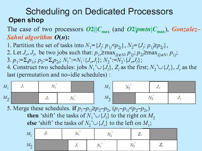
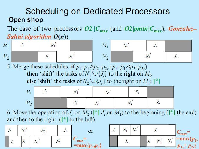
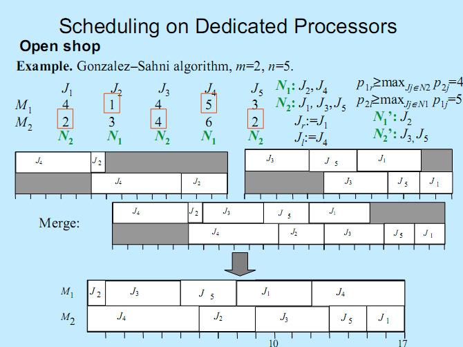
91 Scheduling on Dedicated Processors Flow shop Two processors scheduling F2 C max (includes the case of preemptive scheduling (F2 pmtn C max ), Johnson algorithm O(n log n): 1. Partition the set of jobs into two subsets N 1 ={Z j : p 1j <p 2j }, N 2 ={Z j : p 1j p 2j }, 2. Sort N 1 in non-decreasing p 1j order and N 2 in non-increasing p 2j order, 3. Schedule all the jobs on both machines in order of the concatenation sequence N 1,N 2. Example. Johnson algorithm, m=2, n=5. Z 1 Z 2 Z 3 Z 4 Z 5 M M N 2 N 1 N 2 N 1 N 2 N 1 : Z 2 Z N 2 : Z 3 Z 1 Z M 1 Z 2 Z 2 Z Z 1 Z 4 3 Z 1 Z 5 M 2 Z Z Z 4 Z 3 Z 1 Z
92 Scheduling on Dedicated Processors Flow shop F2 ΣC j is NP-hard, F3 C max, in the case M 2 is dominated by M 1 ( i,j p 1i p 2j ) or by M 3 ( i,j p 3i p 2j ) one can use Johnson algorithm for n jobs with processing times (p 1i +p 2i, p 2i +p 3i ), i=1,...,n. F C max : polynomial-time graphical algorithm for n=2 jobs and arbitrary number of machines. Sketch: 1. We put intervals of the length p 11, p 21,..., p m1 (processing times of J 1 ) on the OX axis and we put invervals of the length p 12, p 22,..., p m2 on the OY axis. 2. We create rectangular obstacles Cartesian products of corresponding intervals (a processor cannot process two tasks at a time). 3. We construct the shortest path consisting of segments parallel to one of the axis (single processor is working) or diagonal in the plane (both processors are working), avoiding passing through any obstacles, from (0,0) to (Σ i p i1, Σ i p i2 ) the distance function is defined by d((x 1,x 2 ),(y 1,y 2 )) = max { x 1 x 2, y 1 y 2 }. The length of the path is qeual to the length of the optimim schedule.
93 Scheduling on Dedicated Processors Flow shop Example. Graphical algorithm. Z m=4, n=2 and 10 2 Z 1 processing times (1,4,4,1); Z 2 processing times (4,1,1,4) Z 1 M 1 Z 1 Z 2 M 1 Z 1 Z 2 M 2 Z 1 Z 2 M 2 Z 1 Z 2 M 3 Z 1 Z 2 M 3 Z 2 Z 1 M 4 Z 1 Z 2 M 4 Z 1 Z
94 Scheduling on Dedicated Processors Open shop The three processors case (O3 C max ) is NP-hard. Proof. PP O3 C max reduction: put n tasks with processing times (0,a i,0) i=1,...,n and three tasks of processing times (S/2,1,S/2), (S/2+1,0,0), (0,0,S/2+1). Determine if there exisits a schedule with C max S+1. M 1 S/2 S/2+1 M 1 S/2+1 S/2 M 2 M 3 a i... 1 a j... S/2+1 S/2 or M 2 M 3 a i... 1 a j... S/2 S/2+1 S+1 S+1 The problem O2 ΣC j is NP-hard.
95
96
97
98 Scheduling on Dedicated Processors Open shop Zero or unit processint times (O ZUET C max ): polynomial-time algorithm based on edge-coloring of bipartite graphs. 1. Bipartite graph G: a) one partition correspond to the job set; the other represents the processors, b) each non-empty operation O ij corresponds to an edge {Z j,m i }. Z 1 Z j Z n M 1 M i M m 2. We edge-color this graph using (G) colors. The colors are interpreted as the time units in which the corresponding tasks are scheduled, (proposal: feasible schedule proper coloring). 3. Then C max *= (G) =max{max i Σ j=1,...,n p ij,max j Σ i=1,...,m p ij }. Obviously, no shorter schedule exists.
99 Scheduling on Dedicated Processors Open shop Preemptive scheduling (O pmtn C max ): pseudo-polynomial algorithm similar to the algorithm for O ZUET C max. We construct a bipartite multigraph G, i.e. each non-empty task T ij corresponds to p ij parallel edges. Again C max * =max{max i Σ j=1,...,n p ij,max j Σ i=1,...,m p ij }. Why pseudo? The number of edges may be non-polynomial (=Σ i=1,...,m; j=1,...,n p ij ), the schedule may contain non-polynomial number of interrupts. Example. Preemptive scheduling m=3, n=5, p 1 =(2,3,0), p 2 =(1,1,1), p 3 =(2,2,2), p 4 =(0,1,3), p 5 =(1,0,1). M 1 M 2 M 3 Z 1 Z 2 Z 3 Z 4 Z 5
100 Scheduling on Dedicated Processors Open shop Preemptive scheduling (O pmtn C max ): pseudo-polynomial algorithm similar to the algorithm for O ZUET C max. We construct a bipartite multigraph G, i.e. each non-empty task T ij corresponds to p ij parallel edges. Again C max * =max{max i Σ j=1,...,n p ij,max j Σ i=1,...,m p ij }. Why pseudo? The number of edges may be non-polynomial (=Σ i=1,...,m; j=1,...,n p ij ), the schedule may contain non-polynomial number of interrupts. Example. Preemptive scheduling m=3, n=5, p 1 =(2,3,0), p 2 =(1,1,1), p 3 =(2,2,2), p 4 =(0,1,3), p 5 =(1,0,1). M 1 M 2 M 3 M 3 Z 3 Z 2 Z 3 Z 4 Z 5 M 2 Z 2 Z 3 Z 1 Z 3 Z 4 M 1 Z 1 Z 3 Z 2 Z 5 Z 1 Z 2 Z 3 Z 4 Z 5 7
101 Scheduling on Dedicated Processors Open shop Preemptive scheduling (O pmtn C max ): polynomial time algorithm is known; it is based on fractional edge-coloring of weighted graph (each task T ij corresponds to an edge {J j,m i } of weight p ij in graph G), Minimizing C max on parallel processors... again Polynomial-time algorithm for R pmtn C max. R pmtn C max O pmtn C max. reduction: Let x ij be the part of T j processed by M i (in the time t ij = p ij x ij ). If we knew optimal values x ij, we could use the above algorithm treating these tasks parts as tasks of preemptive jobs (constraints for the schedule are the same!). How to derive these values? We transform the scheduling problem to linear programming: minimize C such that: Σ i=1,...,m x ij =1, j=1,...,n C Σ j=1,...,n p ij x ij, i=1,...,m, C Σ i=1,...,m p ij x ij, j=1,...,n.
Algorithm Design. Scheduling Algorithms. Part 2. Parallel machines. Open-shop Scheduling. Job-shop Scheduling.
 Algorithm Design Scheduling Algorithms Part 2 Parallel machines. Open-shop Scheduling. Job-shop Scheduling. 1 Parallel Machines n jobs need to be scheduled on m machines, M 1,M 2,,M m. Each machine can
Embedded Systems 15. REVIEW: Aperiodic scheduling. C i J i 0 a i s i f i d i
 Embedded Systems 15-1 - REVIEW: Aperiodic scheduling C i J i 0 a i s i f i d i Given: A set of non-periodic tasks {J 1,, J n } with arrival times a i, deadlines d i, computation times C i precedence constraints
Recoverable Robustness in Scheduling Problems
 Master Thesis Computing Science Recoverable Robustness in Scheduling Problems Author: J.M.J. Stoef (3470997) J.M.J.Stoef@uu.nl Supervisors: dr. J.A. Hoogeveen J.A.Hoogeveen@uu.nl dr. ir. J.M. van den Akker
Partition is reducible to P2 C max. c. P2 Pj = 1, prec Cmax is solvable in polynomial time. P Pj = 1, prec Cmax is NP-hard
 I. Minimizing Cmax (Nonpreemptive) a. P2 C max is NP-hard. Partition is reducible to P2 C max b. P Pj = 1, intree Cmax P Pj = 1, outtree Cmax are both solvable in polynomial time. c. P2 Pj = 1, prec Cmax
Resource Management in Machine Scheduling Problems: A Survey
 Decision Making in Manufacturing and Services Vol. 1 2007 No. 1 2 pp. 59 89 Resource Management in Machine Scheduling Problems: A Survey Adam Janiak,WładysławJaniak, Maciej Lichtenstein Abstract. The paper
Metode şi Algoritmi de Planificare (MAP) Curs 2 Introducere în problematica planificării
 Curs 2 Introducere în problematica planificării") Metode şi Algoritmi de Planificare (MAP) 2009-2010 Curs 2 Introducere în problematica planificării 20.10.2009 Metode si Algoritmi de Planificare Curs 2 1 Introduction to scheduling Scheduling problem definition
Metode şi Algoritmi de Planificare (MAP) 2009-2010 Curs 2 Introducere în problematica planificării 20.10.2009 Metode si Algoritmi de Planificare Curs 2 1 Introduction to scheduling Scheduling problem definition
Embedded Systems 14. Overview of embedded systems design
 Embedded Systems 14-1 - Overview of embedded systems design - 2-1 Point of departure: Scheduling general IT systems In general IT systems, not much is known about the computational processes a priori The
P C max. NP-complete from partition. Example j p j What is the makespan on 2 machines? 3 machines? 4 machines?
 Multiple Machines Model Multiple Available resources people time slots queues networks of computers Now concerned with both allocation to a machine and ordering on that machine. P C max NP-complete from
Scheduling Lecture 1: Scheduling on One Machine
 Scheduling Lecture 1: Scheduling on One Machine Loris Marchal October 16, 2012 1 Generalities 1.1 Definition of scheduling allocation of limited resources to activities over time activities: tasks in computer
Task Models and Scheduling
 Task Models and Scheduling Jan Reineke Saarland University June 27 th, 2013 With thanks to Jian-Jia Chen at KIT! Jan Reineke Task Models and Scheduling June 27 th, 2013 1 / 36 Task Models and Scheduling
CS521 CSE IITG 11/23/2012
 Today Scheduling: lassification Ref: Scheduling lgorithm Peter rukerook Multiprocessor Scheduling : List PTS Ref job scheduling, by uwe schweigelshohn Tomorrow istributed Scheduling ilk Programming and
Lecture 4 Scheduling 1
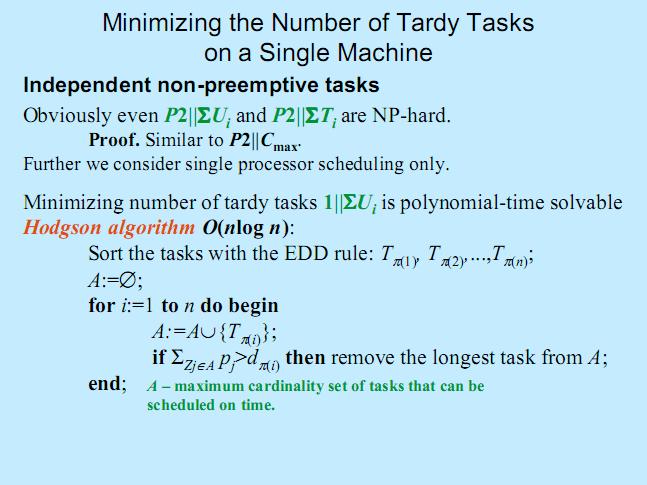
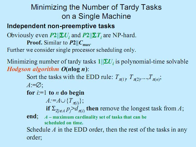
 Lecture 4 Scheduling 1 Single machine models: Number of Tardy Jobs -1- Problem 1 U j : Structure of an optimal schedule: set S 1 of jobs meeting their due dates set S 2 of jobs being late jobs of S 1 are
On Machine Dependency in Shop Scheduling
 On Machine Dependency in Shop Scheduling Evgeny Shchepin Nodari Vakhania Abstract One of the main restrictions in scheduling problems are the machine (resource) restrictions: each machine can perform at
Scheduling Lecture 1: Scheduling on One Machine
 Scheduling Lecture 1: Scheduling on One Machine Loris Marchal 1 Generalities 1.1 Definition of scheduling allocation of limited resources to activities over time activities: tasks in computer environment,
Polynomially solvable and NP-hard special cases for scheduling with heads and tails
 Polynomially solvable and NP-hard special cases for scheduling with heads and tails Elisa Chinos, Nodari Vakhania Centro de Investigación en Ciencias, UAEMor, Mexico Abstract We consider a basic single-machine
Flow Shop and Job Shop Models
 Outline DM87 SCHEDULING, TIMETABLING AND ROUTING Lecture 11 Flow Shop and Job Shop Models 1. Flow Shop 2. Job Shop Marco Chiarandini DM87 Scheduling, Timetabling and Routing 2 Outline Resume Permutation
Single Machine Models
 Outline DM87 SCHEDULING, TIMETABLING AND ROUTING Lecture 8 Single Machine Models 1. Dispatching Rules 2. Single Machine Models Marco Chiarandini DM87 Scheduling, Timetabling and Routing 2 Outline Dispatching
Single Machine Problems Polynomial Cases
 DM204, 2011 SCHEDULING, TIMETABLING AND ROUTING Lecture 2 Single Machine Problems Polynomial Cases Marco Chiarandini Department of Mathematics & Computer Science University of Southern Denmark Outline
Deterministic Models: Preliminaries
 Chapter 2 Deterministic Models: Preliminaries 2.1 Framework and Notation......................... 13 2.2 Examples... 20 2.3 Classes of Schedules... 21 2.4 Complexity Hierarchy... 25 Over the last fifty
RCPSP Single Machine Problems
 DM204 Spring 2011 Scheduling, Timetabling and Routing Lecture 3 Single Machine Problems Marco Chiarandini Department of Mathematics & Computer Science University of Southern Denmark Outline 1. Resource
Lecture 13. Real-Time Scheduling. Daniel Kästner AbsInt GmbH 2013
 Lecture 3 Real-Time Scheduling Daniel Kästner AbsInt GmbH 203 Model-based Software Development 2 SCADE Suite Application Model in SCADE (data flow + SSM) System Model (tasks, interrupts, buses, ) SymTA/S
Lecture 2: Scheduling on Parallel Machines
 Lecture 2: Scheduling on Parallel Machines Loris Marchal October 17, 2012 Parallel environment alpha in Graham s notation): P parallel identical Q uniform machines: each machine has a given speed speed
Minimizing Mean Flowtime and Makespan on Master-Slave Systems
 Minimizing Mean Flowtime and Makespan on Master-Slave Systems Joseph Y-T. Leung,1 and Hairong Zhao 2 Department of Computer Science New Jersey Institute of Technology Newark, NJ 07102, USA Abstract The
CIS 4930/6930: Principles of Cyber-Physical Systems
 CIS 4930/6930: Principles of Cyber-Physical Systems Chapter 11 Scheduling Hao Zheng Department of Computer Science and Engineering University of South Florida H. Zheng (CSE USF) CIS 4930/6930: Principles
Embedded Systems Development
 Embedded Systems Development Lecture 3 Real-Time Scheduling Dr. Daniel Kästner AbsInt Angewandte Informatik GmbH kaestner@absint.com Model-based Software Development Generator Lustre programs Esterel programs
ECS122A Handout on NP-Completeness March 12, 2018
 ECS122A Handout on NP-Completeness March 12, 2018 Contents: I. Introduction II. P and NP III. NP-complete IV. How to prove a problem is NP-complete V. How to solve a NP-complete problem: approximate algorithms
arxiv: v2 [cs.ds] 27 Nov 2014
![arxiv: v2 [cs.ds] 27 Nov 2014](/thumbs/86/93669443.jpg "arxiv: v2 [cs.ds] 27 Nov 2014") Single machine scheduling problems with uncertain parameters and the OWA criterion arxiv:1405.5371v2 [cs.ds] 27 Nov 2014 Adam Kasperski Institute of Industrial Engineering and Management, Wroc law University
Single machine scheduling problems with uncertain parameters and the OWA criterion arxiv:1405.5371v2 [cs.ds] 27 Nov 2014 Adam Kasperski Institute of Industrial Engineering and Management, Wroc law University
Complexity of preemptive minsum scheduling on unrelated parallel machines Sitters, R.A.
 Complexity of preemptive minsum scheduling on unrelated parallel machines Sitters, R.A. Published: 01/01/2003 Document Version Publisher s PDF, also known as Version of Record (includes final page, issue
APTAS for Bin Packing
 APTAS for Bin Packing Bin Packing has an asymptotic PTAS (APTAS) [de la Vega and Leuker, 1980] For every fixed ε > 0 algorithm outputs a solution of size (1+ε)OPT + 1 in time polynomial in n APTAS for
Complexity analysis of the discrete sequential search problem with group activities
 Complexity analysis of the discrete sequential search problem with group activities Coolen K, Talla Nobibon F, Leus R. KBI_1313 Complexity analysis of the discrete sequential search problem with group
MINIMIZING SCHEDULE LENGTH OR MAKESPAN CRITERIA FOR PARALLEL PROCESSOR SCHEDULING
 MINIMIZING SCHEDULE LENGTH OR MAKESPAN CRITERIA FOR PARALLEL PROCESSOR SCHEDULING By Ali Derbala University of Blida, Faculty of science Mathematics Department BP 270, Route de Soumaa, Blida, Algeria.
Scheduling jobs on two uniform parallel machines to minimize the makespan
 UNLV Theses, Dissertations, Professional Papers, and Capstones 5-1-2013 Scheduling jobs on two uniform parallel machines to minimize the makespan Sandhya Kodimala University of Nevada, Las Vegas, kodimalasandhya@gmail.com
Two Processor Scheduling with Real Release Times and Deadlines
 Two Processor Scheduling with Real Release Times and Deadlines Hui Wu School of Computing National University of Singapore 3 Science Drive 2, Singapore 117543 wuh@comp.nus.edu.sg Joxan Jaffar School of
University of Twente. Faculty of Mathematical Sciences. Scheduling split-jobs on parallel machines. University for Technical and Social Sciences
 Faculty of Mathematical Sciences University of Twente University for Technical and Social Sciences P.O. Box 217 7500 AE Enschede The Netherlands Phone: +31-53-4893400 Fax: +31-53-4893114 Email: memo@math.utwente.nl
Real-Time Systems. Lecture 4. Scheduling basics. Task scheduling - basic taxonomy Basic scheduling techniques Static cyclic scheduling
 Real-Time Systems Lecture 4 Scheduling basics Task scheduling - basic taxonomy Basic scheduling techniques Static cyclic scheduling 1 Last lecture (3) Real-time kernels The task states States and transition
Computers and Intractability. The Bandersnatch problem. The Bandersnatch problem. The Bandersnatch problem. A Guide to the Theory of NP-Completeness
 Computers and Intractability A Guide to the Theory of NP-Completeness The Bible of complexity theory Background: Find a good method for determining whether or not any given set of specifications for a
Computers and Intractability
 Computers and Intractability A Guide to the Theory of NP-Completeness The Bible of complexity theory M. R. Garey and D. S. Johnson W. H. Freeman and Company, 1979 The Bandersnatch problem Background: Find
Minimizing total weighted tardiness on a single machine with release dates and equal-length jobs
 Minimizing total weighted tardiness on a single machine with release dates and equal-length jobs G. Diepen J.M. van den Akker J.A. Hoogeveen institute of information and computing sciences, utrecht university
Single Machine Scheduling with Generalized Total Tardiness Objective Function
 Single Machine Scheduling with Generalized Total Tardiness Objective Function Evgeny R. Gafarov a, Alexander A. Lazarev b Institute of Control Sciences of the Russian Academy of Sciences, Profsoyuznaya
Techniques for Proving Approximation Ratios in Scheduling
 Techniques for Proving Approximation Ratios in Scheduling by Peruvemba Sundaram Ravi A thesis presented to the University of Waterloo in fulfillment of the thesis requirement for the degree of Master of
arxiv: v2 [cs.dm] 2 Mar 2017
![arxiv: v2 [cs.dm] 2 Mar 2017](/thumbs/72/66576190.jpg "arxiv: v2 [cs.dm] 2 Mar 2017") Shared multi-processor scheduling arxiv:607.060v [cs.dm] Mar 07 Dariusz Dereniowski Faculty of Electronics, Telecommunications and Informatics, Gdańsk University of Technology, Gdańsk, Poland Abstract
Shared multi-processor scheduling arxiv:607.060v [cs.dm] Mar 07 Dariusz Dereniowski Faculty of Electronics, Telecommunications and Informatics, Gdańsk University of Technology, Gdańsk, Poland Abstract
Shop problems in scheduling
 UNLV Theses, Dissertations, Professional Papers, and Capstones 5-2011 Shop problems in scheduling James Andro-Vasko University of Nevada, Las Vegas Follow this and additional works at: https://digitalscholarship.unlv.edu/thesesdissertations
Scheduling jobs with agreeable processing times and due dates on a single batch processing machine
 Theoretical Computer Science 374 007 159 169 www.elsevier.com/locate/tcs Scheduling jobs with agreeable processing times and due dates on a single batch processing machine L.L. Liu, C.T. Ng, T.C.E. Cheng
SUPPLY CHAIN SCHEDULING: ASSEMBLY SYSTEMS. Zhi-Long Chen. Nicholas G. Hall
 SUPPLY CHAIN SCHEDULING: ASSEMBLY SYSTEMS Zhi-Long Chen Nicholas G. Hall University of Pennsylvania The Ohio State University December 27, 2000 Abstract We study the issue of cooperation in supply chain
Multi-agent scheduling on a single machine to minimize total weighted number of tardy jobs
 This is the Pre-Published Version. Multi-agent scheduling on a single machine to minimize total weighted number of tardy obs T.C.E. Cheng 1, C.T. Ng 1 and J.J. Yuan 2 1 Department of Logistics, The Hong
Scheduling Periodic Real-Time Tasks on Uniprocessor Systems. LS 12, TU Dortmund
 Scheduling Periodic Real-Time Tasks on Uniprocessor Systems Prof. Dr. Jian-Jia Chen LS 12, TU Dortmund 08, Dec., 2015 Prof. Dr. Jian-Jia Chen (LS 12, TU Dortmund) 1 / 38 Periodic Control System Pseudo-code
Lower Bounds for Parallel Machine Scheduling Problems
 Lower Bounds for Parallel Machine Scheduling Problems Philippe Baptiste 1, Antoine Jouglet 2, David Savourey 2 1 Ecole Polytechnique, UMR 7161 CNRS LIX, 91128 Palaiseau, France philippe.baptiste@polytechnique.fr
NP-Completeness. NP-Completeness 1
 NP-Completeness Reference: Computers and Intractability: A Guide to the Theory of NP-Completeness by Garey and Johnson, W.H. Freeman and Company, 1979. NP-Completeness 1 General Problems, Input Size and
Single Machine Scheduling with a Non-renewable Financial Resource
 Single Machine Scheduling with a Non-renewable Financial Resource Evgeny R. Gafarov a, Alexander A. Lazarev b Institute of Control Sciences of the Russian Academy of Sciences, Profsoyuznaya st. 65, 117997
1 Ordinary Load Balancing
 Comp 260: Advanced Algorithms Prof. Lenore Cowen Tufts University, Spring 208 Scribe: Emily Davis Lecture 8: Scheduling Ordinary Load Balancing Suppose we have a set of jobs each with their own finite
On bilevel machine scheduling problems
 Noname manuscript No. (will be inserted by the editor) On bilevel machine scheduling problems Tamás Kis András Kovács Abstract Bilevel scheduling problems constitute a hardly studied area of scheduling
Scheduling with Constraint Programming. Job Shop Cumulative Job Shop
 Scheduling with Constraint Programming Job Shop Cumulative Job Shop CP vs MIP: Task Sequencing We need to sequence a set of tasks on a machine Each task i has a specific fixed processing time p i Each
NP-Completeness. f(n) \ n n sec sec sec. n sec 24.3 sec 5.2 mins. 2 n sec 17.9 mins 35.
 \ n n sec sec sec. n sec 24.3 sec 5.2 mins. 2 n sec 17.9 mins 35.") NP-Completeness Reference: Computers and Intractability: A Guide to the Theory of NP-Completeness by Garey and Johnson, W.H. Freeman and Company, 1979. NP-Completeness 1 General Problems, Input Size and
NP-Completeness Reference: Computers and Intractability: A Guide to the Theory of NP-Completeness by Garey and Johnson, W.H. Freeman and Company, 1979. NP-Completeness 1 General Problems, Input Size and
Embedded Systems - FS 2018
 Institut für Technische Informatik und Kommunikationsnetze Prof. L. Thiele Embedded Systems - FS 2018 Sample solution to Exercise 3 Discussion Date: 11.4.2018 Aperiodic Scheduling Task 1: Earliest Deadline
Ideal preemptive schedules on two processors
 Acta Informatica 39, 597 612 (2003) Digital Object Identifier (DOI) 10.1007/s00236-003-0119-6 c Springer-Verlag 2003 Ideal preemptive schedules on two processors E.G. Coffman, Jr. 1, J. Sethuraman 2,,
Real-Time Systems. Event-Driven Scheduling
 Real-Time Systems Event-Driven Scheduling Marcus Völp, Hermann Härtig WS 2013/14 Outline mostly following Jane Liu, Real-Time Systems Principles Scheduling EDF and LST as dynamic scheduling methods Fixed
Average-Case Performance Analysis of Online Non-clairvoyant Scheduling of Parallel Tasks with Precedence Constraints
 Average-Case Performance Analysis of Online Non-clairvoyant Scheduling of Parallel Tasks with Precedence Constraints Keqin Li Department of Computer Science State University of New York New Paltz, New
The polynomial solvability of selected bicriteria scheduling problems on parallel machines with equal length jobs and release dates
 The polynomial solvability of selected bicriteria scheduling problems on parallel machines with equal length jobs and release dates Hari Balasubramanian 1, John Fowler 2, and Ahmet Keha 2 1: Department
Online Appendix for Coordination of Outsourced Operations at a Third-Party Facility Subject to Booking, Overtime, and Tardiness Costs
 Submitted to Operations Research manuscript OPRE-2009-04-180 Online Appendix for Coordination of Outsourced Operations at a Third-Party Facility Subject to Booking, Overtime, and Tardiness Costs Xiaoqiang
1.1 P, NP, and NP-complete
 CSC5160: Combinatorial Optimization and Approximation Algorithms Topic: Introduction to NP-complete Problems Date: 11/01/2008 Lecturer: Lap Chi Lau Scribe: Jerry Jilin Le This lecture gives a general introduction
Algorithms Design & Analysis. Approximation Algorithm
 Algorithms Design & Analysis Approximation Algorithm Recap External memory model Merge sort Distribution sort 2 Today s Topics Hard problem Approximation algorithms Metric traveling salesman problem A
Marjan van den Akker. Han Hoogeveen Jules van Kempen
 Parallel machine scheduling through column generation: minimax objective functions, release dates, deadlines, and/or generalized precedence constraints Marjan van den Akker Han Hoogeveen Jules van Kempen
Chapter 11. Approximation Algorithms. Slides by Kevin Wayne Pearson-Addison Wesley. All rights reserved.
 Chapter 11 Approximation Algorithms Slides by Kevin Wayne. Copyright @ 2005 Pearson-Addison Wesley. All rights reserved. 1 Approximation Algorithms Q. Suppose I need to solve an NP-hard problem. What should
Multiprocessor Scheduling I: Partitioned Scheduling. LS 12, TU Dortmund
 Multiprocessor Scheduling I: Partitioned Scheduling Prof. Dr. Jian-Jia Chen LS 12, TU Dortmund 22/23, June, 2015 Prof. Dr. Jian-Jia Chen (LS 12, TU Dortmund) 1 / 47 Outline Introduction to Multiprocessor
Basic Scheduling Problems with Raw Material Constraints
 Basic Scheduling Problems with Raw Material Constraints Alexander Grigoriev, 1 Martijn Holthuijsen, 2 Joris van de Klundert 2 1 Faculty of Economics and Business Administration, University of Maastricht,
Partial job order for solving the two-machine flow-shop minimum-length problem with uncertain processing times
 Preprints of the 13th IFAC Symposium on Information Control Problems in Manufacturing, Moscow, Russia, June 3-5, 2009 Fr-A2.3 Partial job order for solving the two-machine flow-shop minimum-length problem
Scheduling Online Algorithms. Tim Nieberg
 Scheduling Online Algorithms Tim Nieberg General Introduction on-line scheduling can be seen as scheduling with incomplete information at certain points, decisions have to be made without knowing the complete
Using column generation to solve parallel machine scheduling problems with minmax objective functions
 Using column generation to solve parallel machine scheduling problems with minmax objective functions J.M. van den Akker J.A. Hoogeveen Department of Information and Computing Sciences Utrecht University
Approximation Algorithms for scheduling
 Approximation Algorithms for scheduling Ahmed Abu Safia I.D.:119936343, McGill University, 2004 (COMP 760) Approximation Algorithms for scheduling Leslie A. Hall The first Chapter of the book entitled
Lower Bounds for Parallel Machine Scheduling Problems
 Lower Bounds for Parallel Machine Scheduling Problems Philippe Baptiste 1, Antoine Jouglet 2,, David Savourey 2 1 Ecole Polytechnique, UMR 7161 CNRS LIX, 91128 Palaiseau, France philippe.baptiste@polytechnique.fr
A polynomial-time approximation scheme for the two-machine flow shop scheduling problem with an availability constraint
 A polynomial-time approximation scheme for the two-machine flow shop scheduling problem with an availability constraint Joachim Breit Department of Information and Technology Management, Saarland University,
Single Machine Scheduling: Comparison of MIP Formulations and Heuristics for. Interfering Job Sets. Ketan Khowala
 Single Machine Scheduling: Comparison of MIP Formulations and Heuristics for Interfering Job Sets by Ketan Khowala A Dissertation Presented in Partial Fulfillment of the Requirements for the Degree Doctor
Optimal on-line algorithms for single-machine scheduling
 Optimal on-line algorithms for single-machine scheduling J.A. Hoogeveen A.P.A. Vestjens Department of Mathematics and Computing Science, Eindhoven University of Technology, P.O.Box 513, 5600 MB, Eindhoven,
HYBRID FLOW-SHOP WITH ADJUSTMENT
 K Y BERNETIKA VOLUM E 47 ( 2011), NUMBER 1, P AGES 50 59 HYBRID FLOW-SHOP WITH ADJUSTMENT Jan Pelikán The subject of this paper is a flow-shop based on a case study aimed at the optimisation of ordering
ALG 5.4. Lexicographical Search: Applied to Scheduling Theory. Professor John Reif
 Algorithms Professor John Reif ALG 54 input assume problem Scheduling Problems Set of n tasks in precidence relation on tasks Also, given m processors Unit time cost to process task using single processor
End-to-End Scheduling to Meet Deadlines in Distributed Systems
 Appeared in: Proceedings of the 12th International Conference on Distributed Computing Systems, Yokohama, Japan, June 1992, pages 452--459. End-to-End Scheduling to Meet Deadlines in Distributed Systems
CMSC 722, AI Planning. Planning and Scheduling
 CMSC 722, AI Planning Planning and Scheduling Dana S. Nau University of Maryland 1:26 PM April 24, 2012 1 Scheduling Given: actions to perform set of resources to use time constraints» e.g., the ones computed
3. Scheduling issues. Common approaches 3. Common approaches 1. Preemption vs. non preemption. Common approaches 2. Further definitions
 Common approaches 3 3. Scheduling issues Priority-driven (event-driven) scheduling This class of algorithms is greedy They never leave available processing resources unutilized An available resource may
Study of Scheduling Problems with Machine Availability Constraint
 Journal of Industrial and Systems Engineering Vol. 1, No. 4, pp 360-383 Winter 2008 Study of Scheduling Problems with Machine Availability Constraint Hamid Reza Dehnar Saidy 1*, Mohammad Taghi Taghavi-Fard
Algorithms. Outline! Approximation Algorithms. The class APX. The intelligence behind the hardware. ! Based on
 6117CIT - Adv Topics in Computing Sci at Nathan 1 Algorithms The intelligence behind the hardware Outline! Approximation Algorithms The class APX! Some complexity classes, like PTAS and FPTAS! Illustration
Contents college 5 and 6 Branch and Bound; Beam Search (Chapter , book)! general introduction
! general introduction") Contents college 5 and 6 Branch and Bound; Beam Search (Chapter 3.4-3.5, book)! general introduction Job Shop Scheduling (Chapter 5.1-5.3, book) ffl branch and bound (5.2) ffl shifting bottleneck heuristic
Contents college 5 and 6 Branch and Bound; Beam Search (Chapter 3.4-3.5, book)! general introduction Job Shop Scheduling (Chapter 5.1-5.3, book) ffl branch and bound (5.2) ffl shifting bottleneck heuristic
EECS 571 Principles of Real-Time Embedded Systems. Lecture Note #7: More on Uniprocessor Scheduling
 EECS 571 Principles of Real-Time Embedded Systems Lecture Note #7: More on Uniprocessor Scheduling Kang G. Shin EECS Department University of Michigan Precedence and Exclusion Constraints Thus far, we
Dynamic Scheduling with Genetic Programming
 Dynamic Scheduling with Genetic Programming Domago Jakobović, Leo Budin domago.akobovic@fer.hr Faculty of electrical engineering and computing University of Zagreb Introduction most scheduling problems
Scheduling with Common Due Date, Earliness and Tardiness Penalties for Multi-Machine Problems: A Survey
 Scheduling with Common Due Date, Earliness and Tardiness Penalties for Multi-Machine Problems: A Survey Volker Lauff and Frank Werner 1 Otto-von-Guericke-Universität, Fakultät für Mathematik, PSF 4120,
Chapter 11. Approximation Algorithms. Slides by Kevin Wayne Pearson-Addison Wesley. All rights reserved.
 Chapter 11 Approximation Algorithms Slides by Kevin Wayne. Copyright @ 2005 Pearson-Addison Wesley. All rights reserved. 1 P and NP P: The family of problems that can be solved quickly in polynomial time.
CS360 Homework 12 Solution
 CS360 Homework 12 Solution Constraint Satisfaction 1) Consider the following constraint satisfaction problem with variables x, y and z, each with domain {1, 2, 3}, and constraints C 1 and C 2, defined
CMSC 451: Lecture 7 Greedy Algorithms for Scheduling Tuesday, Sep 19, 2017
 CMSC CMSC : Lecture Greedy Algorithms for Scheduling Tuesday, Sep 9, 0 Reading: Sects.. and. of KT. (Not covered in DPV.) Interval Scheduling: We continue our discussion of greedy algorithms with a number
Unit 1A: Computational Complexity
 Unit 1A: Computational Complexity Course contents: Computational complexity NP-completeness Algorithmic Paradigms Readings Chapters 3, 4, and 5 Unit 1A 1 O: Upper Bounding Function Def: f(n)= O(g(n)) if
Networked Embedded Systems WS 2016/17
 Networked Embedded Systems WS 2016/17 Lecture 2: Real-time Scheduling Marco Zimmerling Goal of Today s Lecture Introduction to scheduling of compute tasks on a single processor Tasks need to finish before
Decision Diagrams for Sequencing and Scheduling
 Decision Diagrams for Sequencing and Scheduling Willem-Jan van Hoeve Tepper School of Business Carnegie Mellon University www.andrew.cmu.edu/user/vanhoeve/mdd/ Plan What can MDDs do for Combinatorial Optimization?
Chapter 3: Discrete Optimization Integer Programming
 Chapter 3: Discrete Optimization Integer Programming Edoardo Amaldi DEIB Politecnico di Milano edoardo.amaldi@polimi.it Website: http://home.deib.polimi.it/amaldi/opt-16-17.shtml Academic year 2016-17
Scheduling on Unrelated Parallel Machines. Approximation Algorithms, V. V. Vazirani Book Chapter 17
 Scheduling on Unrelated Parallel Machines Approximation Algorithms, V. V. Vazirani Book Chapter 17 Nicolas Karakatsanis, 2008 Description of the problem Problem 17.1 (Scheduling on unrelated parallel machines)
RUN-TIME EFFICIENT FEASIBILITY ANALYSIS OF UNI-PROCESSOR SYSTEMS WITH STATIC PRIORITIES
 RUN-TIME EFFICIENT FEASIBILITY ANALYSIS OF UNI-PROCESSOR SYSTEMS WITH STATIC PRIORITIES Department for Embedded Systems/Real-Time Systems, University of Ulm {name.surname}@informatik.uni-ulm.de Abstract:
Friday Four Square! Today at 4:15PM, Outside Gates
 P and NP Friday Four Square! Today at 4:15PM, Outside Gates Recap from Last Time Regular Languages DCFLs CFLs Efficiently Decidable Languages R Undecidable Languages Time Complexity A step of a Turing
CS 580: Algorithm Design and Analysis. Jeremiah Blocki Purdue University Spring 2018
 CS 580: Algorithm Design and Analysis Jeremiah Blocki Purdue University Spring 2018 Chapter 9 PSPACE: A Class of Problems Beyond NP Slides by Kevin Wayne. Copyright @ 2005 Pearson-Addison Wesley. All rights
1 Basic Definitions. 2 Proof By Contradiction. 3 Exchange Argument
 1 Basic Definitions A Problem is a relation from input to acceptable output. For example, INPUT: A list of integers x 1,..., x n OUTPUT: One of the three smallest numbers in the list An algorithm A solves
LPT rule: Whenever a machine becomes free for assignment, assign that job whose. processing time is the largest among those jobs not yet assigned.
 LPT rule Whenever a machine becomes free for assignment, assign that job whose processing time is the largest among those jobs not yet assigned. Example m1 m2 m3 J3 Ji J1 J2 J3 J4 J5 J6 6 5 3 3 2 1 3 5
Scheduling Parallel Jobs with Linear Speedup
 Scheduling Parallel Jobs with Linear Speedup Alexander Grigoriev and Marc Uetz Maastricht University, Quantitative Economics, P.O.Box 616, 6200 MD Maastricht, The Netherlands. Email: {a.grigoriev, m.uetz}@ke.unimaas.nl
Coin Changing: Give change using the least number of coins. Greedy Method (Chapter 10.1) Attempt to construct an optimal solution in stages.
 Attempt to construct an optimal solution in stages.") IV-0 Definitions Optimization Problem: Given an Optimization Function and a set of constraints, find an optimal solution. Optimal Solution: A feasible solution for which the optimization function has the
IV-0 Definitions Optimization Problem: Given an Optimization Function and a set of constraints, find an optimal solution. Optimal Solution: A feasible solution for which the optimization function has the