UNIT ROOT TESTS, COINTEGRATION, ECM, VECM, AND CAUSALITY MODELS

Transcription

1 UNIT ROOT TESTS, COINTEGRATION, ECM, VECM, AND CAUSALITY MODELS Compiled by M&B EFA is desroying he brains of curren generaion s researchers in his counry. Please sop i as much as you can. Thank you. The aim of his lecure is o provide you wih he key conceps of ime series economerics. To is end, you are able o undersand ime-series based researches, officially published in inernaional journals 1 such as applied economics, applied economerics, and he likes. Moreover, I also expec ha some of you will be ineresed in ime series daa analysis, and choose he relaed opics for your fuure hesis. As he ime his lecure is compiled, I believe ha he Vienam ime series daa 2 is long enough for you o conduc such sudies. This is jus a brief summary of he body of knowledge in he field according o my own undersanding. Therefore, i has no scienific value for your ciaions. In addiion, researches using bivariae models have no 1 Seleced papers were compiled by Phung Thanh Binh & Vo Duc Hoang Vu (2009). You can find hem a he H library. 2 The mos imporan daa sources for hese sudies can be World Bank s World Developmen Indicaors, IMF-IFS, GSO, and Reuers Thomson. 1

2 been highly appriciaed by inernaional journal s ediors and my universiy s supervisors. As a researcher, you mus be fully responsible for your own choice in his field of research. My advice is ha you should firsly sar wih he research problem of your ineres, no wih daa you have and saisical echniques you know. A he curren ime, EFA becomes he mos supid phenomenon of young researchers ha I ve ever seen in my universiy of economics, HCMC. They blindly imiae ohers. I don wan he series of models presened in his lecure will become he second wave of research ha annoys he fuure generaion of my universiy. Therefore, jus use i if you really need and undersand i. Some opics such as serial correlaion, ARIMA models, ARCH family models, srucural breaks 3, and panel uni roo and coinegraion ess are beyond he scope of his lecure. You can find hem elsewhere such as economerics exbooks, journal aricles, and my lecure noes in Vienamese. The aim of his lecure is o provide you: An overview of ime series economerics The concep of nonsaionary The concep of spurious regression The uni roo ess The shor-run and long-run relaionships 3 My aricle abou hreshold coinegraion and causaliy analysis in growh-energy consumpion nexus ( did menion abou his issue. 2

3 Auoregressive disribued lag (ARDL) model and error correcion model (ECM) Single-equaion esimaion of he ECM using he Engle-Granger 2-sep mehod Vecor auoregressive (VAR) models Granger causaliy ess (boh coinegraed and noncoinegraed series) Esimaing a sysem of ECMs using vecor error correcion model (VECM) Opimal lag lengh selecion crieria ARDL and bounds es for coinegraion Basic pracicaliies in using Eviews and Saa Suggesed research opics 1. AN OVERVIEW OF TIME SERIES ECONOMETRICS In his lecure, we will mainly discuss single equaion esimaion echniques in a very differen way from wha you have previously learned in he basic economerics course. According o Aseriou (2007), here are various aspecs o ime series analysis bu he mos common heme o hem is o fully exploi he dynamic srucure in he daa. Saying differenly, we will exrac as much informaion as possible from he pas hisory of he series. The analysis of ime series is usually explored wihin wo fundamenal ypes, namely, ime series forecasing and dynamic modelling. Pure ime series forecasing, such as ARIMA and ARCH/GARCH family models, is ofen menioned as univariae analysis. Unlike mos oher economerics, in univariae analysis we do no 3

4 concern much wih building srucural models, undersanding he economy or esing hypohesis, bu wha we really concern is developing efficien models, which are able o forecas well. The efficien forecasing models can be empirically evaluaed using various ways such as significance of he esimaed coefficiens (especially he longes lags in ARIMA), he posiive sign of he coefficiens in ARCH, diagnosic checking using he correlogram, Akaike and Schwarz crieria, and graphics. In hese cases, we ry o exploi he dynamic iner-relaionship, which exiss over ime for any single variable (say, asse prices, exchange raes, ineres raes, ec). On he oher hand, dynamic modelling, including bivariae and mulivariae ime series analysis, is mosly concerned wih undersanding he srucure of he economy and esing hypohesis. However, his kind of modelling is based on he view ha mos economic series are slow o adjus o any shock and so o undersand he process mus fully capure he adjusmen process which may be long and complex (Aseriou, 2007). The dynamic modelling has become increasingly popular hanks o he works of wo Nobel laureaes in economics 2003, namely, Granger (for mehods of analyzing economic ime series wih common rends, or coinegraion) and Engle (for mehods of analyzing economic ime series wih ime-varying volailiy or ARCH) 4. Up o now, dynamic 4 hp://nobelprize.org/nobel_prizes/economics/laureaes/2003/ 4

5 modelling has remarkably conribued o economic policy formulaion in various fields. Generally, he key purpose of ime series analysis is o capure and examine he dynamics of he daa. In ime series economerics, i is equally imporan ha he analyss should clearly undersand he erm sochasic process. According o Gujarai (2003), a random or sochasic process is a collecion of random variables ordered in ime. If we le Y denoe a random variable, and if i is coninuous, we denoe i a Y(), bu if i is discree, we denoe i as Y. Since mos economic daa are colleced a discree poins in ime, we usually use he noaion Y raher han Y(). If we le Y represen GDP, we have Y1, Y2, Y3,, Y88, where he subscrip 1 denoes he firs observaion (i.e., GDP for he firs quarer of 1970) and he subscrip 88 denoes he las observaion (i.e., GDP for he fourh quarer of 1991). Keep in mind ha each of hese Y s is a random variable. In wha sense we can regard GDP as a sochasic process? Consider for insance he GDP of $ billion for 1970Q1. In heory, he GDP figure for he firs quarer of 1970 could have been any number, depending on he economic and poliical climae hen prevailing. The figure of $ billion is jus a paricular realizaion of all such possibiliies. In his case, we can hink of he value of $ billion as he mean value of all possible values of GDP for he firs quarer 5

6 of Therefore, we can say ha GDP is a sochasic process and he acual values we observed for he period 1970Q1 o 1991Q4 are a paricular realizaion of ha process. Gujarai (2003) saes ha he disincion beween he sochasic process and is realizaion in ime series daa is jus like he disincion beween populaion and sample in cross-secional daa. Jus as we use sample daa o draw inferences abou a populaion; in ime series, we use he realizaion o draw inferences abou he underlying sochasic process. The reason why I menion his erm before examining specific models is ha all basic assumpions in ime series models relae o he sochasic process (populaion). Sock & Wason (2007) say ha he assumpion ha he fuure will be like he pas is an imporan one in ime series regression. If he fuure is like he pas, hen he hisorical relaionships can be used o forecas he fuure. Bu if he fuure differs fundamenally from he pas, hen he hisorical relaionships migh no be reliable guides o he fuure. Therefore, in he conex of ime series regression, he idea ha hisorical relaionships can be generalized o he fuure is formalized by he concep of saionariy. 2. STATIONARY STOCHASTIC PROCESSES 2.1 Definiion According o Gujarai (2003), a key concep underlying sochasic process ha has received a grea deal of 6

7 aenion and scruiny by ime series analyss is he socalled saionary sochasic process. Broadly speaking, a ime series is said o be saionary if is mean and variance are consan over ime and he value of he covariance 5 beween he wo periods depends only on he disance or gap or lag beween he wo ime periods and no he acual ime a which he covariance is compued (Gujarai, 2011). In he ime series lieraure, such a sochasic process is known as a weakly saionary or covariance saionary. By conras, a ime series is sricly saionary if all he momens of is probabiliy disribuion and no jus he firs wo (i.e., mean and variance) are invarian over ime. If, however, he saionary process is normal, he weakly saionary sochasic process is also sricly saionary, for he normal sochasic process is fully specified by is wo momens, he mean and he variance. For mos pracical siuaions, he weak ype of saionariy ofen suffices. According o Aseriou (2007), a ime series is weakly saionary when i has he following characerisics: (a) (b) (c) exhibis mean reversion in ha i flucuaes around a consan long-run mean; has a finie variance ha is ime-invarian; and has a heoreical correlogram ha diminishes as he lag lengh increases. 5 or he auocorrelaion coefficien. 7

8 In is simples erms a ime series Y is said o be weakly saionary (hereafer refer o saionary) if: (a) Mean: E(Y) = (consan for all ); (b) Variance: Var(Y) = E(Y-) 2 = 2 (consan for all ); and (c) Covariance: Cov(Y,Y+k) = k = E[(Y-)(Y+k-)] where k, covariance (or auocovariance) a lag k, is he covariance beween he values of Y and Y+k, ha is, beween wo Y values k periods apar. If k = 0, we obain 0, which is simply he variance of Y (= 2 ); if k = 1, 1 is he covariance beween wo adjacen values of Y. Suppose we shif he origin of Y from Y o Y+m (say, from he firs quarer of 1970 o he firs quarer of 1975 for our GDP daa). Now, if Y is o be saionary, he mean, variance, and auocovariance of Y+m mus be he same as hose of Y. In shor, if a ime series is saionary, is mean, variance, and auocovariance (a various lags) remain he same no maer a wha poin we measure hem; ha is, hey are ime invarian. According o Gujarai (2003), such ime series will end o reurn o is mean (called mean reversion) and flucuaions around his mean (measured by is variance) will have a broadly consan ampliude. If a ime series is no saionary in he sense jus defined, i is called a nonsaionary ime series. In 8

9 oher words, a nonsaionary ime series will have a ime-varying mean or a ime-varying variance or boh. Why are saionary ime series so imporan? According o Gujarai (2003, 2011), here are a leas wo reasons. Firs, if a ime series is nonsaionary, we can sudy is behavior only for he ime period under consideraion. Each se of ime series daa will herefore be for a paricular episode. As a resul, i is no possible o generalize i o oher ime periods. Therefore, for he purpose of forecasing or policy analysis, such (nonsaionary) ime series may be of lile pracical value. Second, if we have wo or more nonsaionary ime series, regression analysis involving such ime series may lead o he phenomenon of spurious or nonsense regression (Gujarai, 2011; Aseriou, 2007). In addiion, a special ype of sochasic process (or ime series), namely, a purely random, or whie noise, process, is also popular in ime series economerics. According o Gujarai (2003), we call a sochasic process purely random if i has zero mean, consan variance 2, and is serially uncorrelaed. This is similar o wha we call he error erm, u, in he classical normal linear regression model, once discussed in he phenomenon of serial correlaion opic. This error erm is ofen denoed as u ~ iid(0, 2 ). 2.2 Random Walk Process 9

10 According o Sock and Wason (2007), ime series variables can fail o be saionary in various ways, bu wo are especially relevan for regression analysis of economic ime series daa: (1) he series can have persisen, long-run movemens, ha is, he series can have rends; and, (2) he populaion regression can be unsable over ime, ha is, he populaion regression can have breaks. For he purpose of his lecure, I only focus on he firs ype of nonsaionariy. A rend is a persisen long-erm movemen of a variable over ime. A ime series variable flucuaes around is rend. There are wo ypes of rends ofen seen in ime series daa: deerminisic and sochasic. A deerminisic rend is a nonrandom funcion of ime (i.e. Y = A + B*Time + u, Y = A + B*Time + C*Time 2 + u, and so on) 6. For example, he LEX [he logarihm of he dollar/euro daily exchange rae, LEX.wf1, Gujarai (2011)] is a nonsaionary seris (Figure 2.1), and is derended series (i.e. residuals from he regression of log(ex) on ime: e = log(ex) a b*time) is sill nonsaionary (Figure 2.2). This indicaes ha log(ex) is no a rend saionary series. 6 Y = a + bt + e => e = Y a bt is called he derended series. If Y is nonsaionary, while e is saionary, Y is known as he rend (sochasic) saionary (TSP). Here, he process wih a deerminisic rend is nonsaionary bu no a uni roo process. 10

11 Figure 2.1: Log of he dollar/euro daily exchange rae Figure 2.2: Residuals from he regression of LEX on ime. In conras, a sochasic rend is random and varies over ime. According o Sock and Wason (2007), i is more appropriae o model economic ime series as having 11

12 sochasic raher han deerminisic rends. Therefore, our reamen of rends in economic ime series focuses mainly on sochasic raher han deerminisic rends, and when we refer o rends in ime series daa, we mean sochasic rends unless we explicily say oherwise. The simples model of a variable wih a sochasic rend is he random walk. There are wo ypes of random walks: (1) random walk wihou drif (i.e. no consan or inercep erm) and (2) random walk wih drif (i.e. a consan erm is presen). The random walk wihou drif is defined as follow. Suppose u is a whie noise error erm wih mean 0 and variance 2. The Y is said o be a random walk if: Y = Y-1 + u (1) The basic idea of a random walk is ha he value of he series omorrow (Y+1) is is value oday (Y), plus an unpredicable change (u+1). From (1), we can wrie Y1 = Y0 + u1 Y2 = Y1 + u2 = Y0 + u1 + u2 Y3 = Y2 + u3 = Y0 + u1 + u2 + u3 Y4 = Y3 + u4 = Y0 + u1 + + u4 Y = Y-1 + u = Y0 + u1 + + u 12

13 In general, if he process sared a some ime 0 wih a value Y0, we have Y Y0 u (2) herefore, E (Y ) E(Y0 u ) Y0 In like fashion, i can be shown ha Var(Y ) (E Y 0 u 2 0 Y ) (E u 2 ) 2 Therefore, he mean of Y is equal o is iniial or saring value, which is consan, bu as increases, is variance increases indefiniely, hus violaing a condiion of saionariy. In oher words, he variance of Y depends on, is disribuion depends on, ha is, i is nonsaionary. Ineresingly, if we re-wrie (1) as (Y Y-1) = Y = u (3) where Y is he firs difference of Y. I is easy o show ha, while Y is nonsaionary, is firs difference is saionary. And his is very significan when working wih ime series daa. This is widely known as he difference saionary (sochasic) process (DSP). 13

14 Figure 2.3: A random walk wihou drif Figure 2.4: Firs difference of LEX. 14

15 The random walk wih drif can be defined as follow: Y = + Y-1 + u (4) where is known as he drif parameer. The name drif comes from he fac ha if we wrie he preceding equaion as: Y Y-1 = Y = + u (5) i shows ha Y drifs upward or downward, depending on being posiive or negaive. We can easily show ha, he random walk wih drif violaes boh condiions of saionariy: E(Y) = Y0 +. Var(Y) = 2 In oher words, boh mean and variance of Y depends on, is disribuion depends on, ha is, i is nonsaionary. Sock and Wason (2007) say ha because he variance of a random walk increases wihou bound, is populaion auocorrelaions are no defined (he firs auocovariance and variance are infinie and he raio of he wo is no well defined) 7. 7 Corr(Y,Y -1) = Cov(Y,Y ) Var(Y )Var(Y 1 ~ 1 ) 15

16 Figure 2.5: A random walk wih drif (Y = 2 + Y-1 + u) Figure 2.6: Random walk wih drif (Y = -2 + Y-1 + u). 16

17 2.3 Uni Roo Sochasic Process According o Gujarai (2003), he random walk model is an example of wha is known in he lieraure as a uni roo process. Le us wrie he random walk model (1) as: Y = Y-1 + u (-1 1) (6) This model resembles he Markov firs-order auoregressive model [AR(1)], menioned in he basic economerics course, serial correlaion opic. If = 1, (6) becomes a random walk wihou drif. If is in fac 1, we face wha is known as he uni roo problem, ha is, a siuaion of nonsaionariy. The name uni roo is due o he fac ha = 1. Technically, if = 1, we can wrie (6) as Y Y-1 = u. Now using he lag operaor L so ha Ly = Y-1, L 2 Y = Y-2, and so on, we can wrie (6) as (1-L)Y = u. If we se (1-L) = 0, we obain, L = 1, hence he name uni roo. Thus, he erms nonsaionariy, random walk, and uni roo can be reaed as synonymous. If, however, 1, ha is if he absolue value of is less han one, hen i can be shown ha he ime series Y is saionary. 2.4 Illusraive Examples Consider he AR(1) model as presened in equaion (6). Generally, we can have hree possible cases: 17

18 Case 1: < 1 and herefore he series Y is saionary. A graph of a saionary series for = 0.67 is presened in Figure 2.7. Case 2: > 1 where in his case he series explodes. A graph of an explosive series for = 1.26 is presened in Figure 2.8. Case 3: = 1 where in his case he series conains a uni roo and is non-saionary. Graph of saionary series for = 1 are presened in Figure 2.9. In order o reproduce he graphs and he series which are saionary, exploding and nonsaionary, we ype he following commands in Eviews: Sep 1: Open a new workfile (say, undaed ype), conaining 200 observaions. Sep 2: Generae X, Y, Z as he following commands: smpl 1 1 genr X=0 genr Y=0 genr Z=0 smpl genr X=0.67*X(-1)+nrnd genr Y=1.26*Y(-1)+nrnd genr Z=Z(-1)+nrnd 18

19 smpl Sep 3: Plo X, Y, Z using he line plo ype (Figures 2.7, 2.8, and 2.9). plo X plo Y plo Z Figure 2.7: A saionary series 19

20 1.6E E E E E E E E E Figure 2.8: An explosive series Figure 2.9: A nonsaionary series 20

21 3. THE UNIT ROOTS AND SPURIOUS REGRESSIONS 3.1 Spurious Regressions Mos macroeconomic ime series are rended and herefore in mos cases are nonsaionary. The problem wih nonsaionary or rended daa is ha he sandard ordinary leas squares (OLS) regression procedures can easily lead o incorrec conclusions. According o Aseriou (2007), i can be shown in hese cases ha he regression resuls have very high value of R 2 (someimes even higher han 0.95) and very high values of -raios (someimes even higher han 4), while he variables used in he analysis have no real inerrelaionships. Aseriou (2007) saes ha many economic series ypically have an underlying rae of growh, which may or may no be consan, for example GDP, prices or money supply all end o grow a a regular annual rae. Such series are no saionary as he mean is coninually rising however hey are also no inegraed as no amoun of differencing can make hem saionary. This gives rise o one of he main reasons for aking he logarihm of daa before subjecing i o formal economeric analysis. If we ake he logarihm of a series, which exhibis an average growh rae we will urn i ino a series which follows a linear rend and which is inegraed. This can be easily seen formally. Suppose we have a series X, which increases by 10% every period, hus: X = 1.1X-1 21

22 If we hen ake he logarihm of his we ge log(x) = log(1.1) + log(x-1) Now he lagged dependen variable has a uni coefficien and each period i increases by an absolue amoun equal o log(1.1), which is of course consan. This series would now be I(1). More formally, consider he model: Y = β1 + β2x + u (7) where u is he error erm. The assumpions of classical linear regression model (CLRM) require boh Y and X o have zero and consan variance (i.e., o be saionary). In he presence of nonsaionariy, hen he resuls obained from a regression of his kind are oally spurious 8 and hese regressions are called spurious regressions. The inuiion behind his is quie simple. Over ime, we expec any nonsaionary series o wander around (see Figure 3.1), so over any reasonably long sample he series eiher drif up or down. If we hen consider wo compleely unrelaed series which are boh nonsaionary, we would expec ha eiher hey will boh go up or down ogeher, or one will go up while he oher goes down. If we hen performed a regression of one series on he oher, we would hen find eiher a significan posiive 8 This was firs inroduced by Yule (1926), and re-examined by Granger and Newbold (1974) using he Mone Carlo simulaions. 22

23 relaionship if hey are going in he same direcion or a significan negaive one if hey are going in opposie direcions even hough really hey are boh unrelaed. This is he essence of a spurious regression. I is said ha a spurious regression usually has a very high R 2, saisics ha appear o provide significan esimaes, bu he resuls may have no economic meaning. This is because he OLS esimaes may no be consisen, and herefore all he ess of saisical inference are no valid. Granger and Newbold (1974) consruced a Mone Carlo analysis generaing a large number of Y and X series conaining uni roos following he formulas: Y = Y-1 + ey (8) X = X-1 + ex (9) where ey and ex are arificially generaed normal random numbers (as he same way performed in secion 2.4). Since Y and X are independen of each oher, any regression beween hem should give insignifican resuls. However, when hey regressed he various Ys o he Xs as show in equaion (8), hey surprisingly found ha hey were unable o rejec he null hypohesis of β2 = 0 for approximaely 75% of heir cases. They also found ha heir regressions had very high R 2 s and very low values of DW saisics. 23

24 To see he spurious regression problem, we can ype he following commands in Eviews (afer opening he new workfile, say, undaed wih 500 observaions) o see how many imes we can rejec he null hypohesis of β2 = 0. The commands (or smpl 1 1) genr Y=0 genr (or smpl 2 500) genr Y=Y(-1)+nrnd genr X=X(-1)+nrnd sca(r) Y ls Y c X An example of a plo of Y agains X obained in his way is shown in Figure 3.1. The esimaed equaion beween hese wo simulaed series is: Table 3.1: Spurious regression 24

25 Y TOPICS IN TIME SERIES ECONOMETRICS X Figure 3.1: Scaer plo of a spurious regression Granger and Newbold (1974) proposed he following rule of humb for deecing spurious regressions: If R 2 > DW saisic or if R 2 1 hen he esimaed regression mus be spurious. To undersand he problem of spurious regression beer, i migh be useful o use an example wih real economic daa. This example was conduced by Aseriou (2007). Consider a regression of he logarihm of real GDP (Y) o he logarihm of real money supply (M) and a consan. The resuls obained from such a regression are he following: 25

26 Y = M; R 2 = 0.945; DW = (4.743) (8.572) Here we see very good -raios, wih coefficiens ha have he righ signs and more or less plausible magniudes. The coefficien of deerminaion is very high (R 2 = 0.945), bu here is a high degree of auocorrelaion (DW = 0.221). This shows evidence of he possible exisence of spurious regression. In fac, his regression is oally meaningless because he money supply daa are for he UK economy and he GDP figures are for he US economy. Therefore, alhough here should no be any significan relaionship, he regression seems o fi he daa very well, and his happens because he variables used in he example are, simply, rended (i.e. nonsaionary). So, Aseriou (2007) recommends ha economericians should be very careful when working wih rended variables. You can find more such examples in Gujarai (2011, pp ) 3.2 Explaining he Spurious Regression Problem According o Aseriou (2007), in a slighly more formal way he source of he spurious regression problem comes from he fac ha if wo variables, X and Y, are boh saionary, hen in general any linear combinaion of hem will cerainly be saionary. One imporan linear combinaion of hem is of course he equaion error, and so if boh variables are saionary, he error in he equaion will also be saionary and have a well-behaved 26

27 disribuion. However, when he variables become nonsaionary, hen of course we can no guaranee ha he errors will be saionary and in fac as a general rule (alhough no always) he error iself be nonsaionary and when his happens, we violae he basic CLRM assumpions of OLS regression. If he errors were nonsaionary, we would expec hem o wander around and evenually ge large. Bu OLS regression because i selecs he parameers so as o make he sum of he squared errors as small as possible will selec any parameer which gives he smalles error and so almos any parameer value can resul. The simples way o examine he behaviour of u is o rewrie (7) as: u = Y β1 β2x (10) or, excluding he consan β1 (which only affecs u sequence by rescaling i): u = Y β2x (11) If Y and X are generaed by equaions (8) and (9), hen if we impose he iniial condiions Y0 = X0 = 0 we ge ha: u Y 0 e Y1 e Y2... e Yi (X 2 0 e X1 e X2... e Xi ) or u e e (12) i1 Yi 2 i1 Xi 27

28 From equaion (12), we realize ha he variance of he error erm will end o become infiniely large as increases. Hence, he assumpions of he CLRM are violaed, and herefore, any es, F es or R 2 are unreliable. In erms of equaion (7), here are four differen cases o discuss: Case 1: Boh Y and X are saionary 9, and he CLRM is appropriae wih OLS esimaes being BLUE. Case 2: Y and X are inegraed of differen orders. In his case, he regression equaions are meaningless. Case 3: Y and X are inegraed of he same order [ofen I(1)]and he u sequence conains a sochasic rend. In his case, we have spurious regression and i is ofen recommended o re-esimae he regression equaion in he semi-difference mehods (such as he FGLS mehod: Orcu-Cochrane procedure, AR(1), and Newey-Wes sandard error). These mehods did menion in my lecures abou serial correlaion and a brief review of basic economerics. Case 4: Y and X are inegraed of he same order and he u is saionary. In his special case, Y and X 9 Based on he saisical ess such as ADF, PP, and KPSS. 28

29 are said o be coinegraed. The concep of coinegraion will be examined in deail laer. 4. TESTING FOR UNIT ROOTS 4.1 Graphical Analysis According o Gujarai (2003), before one pursues formal ess, i is always advisable o plo he ime series under sudy. Such a plo (line graph of he level) and correlogram [of boh he level (ACF) and he firs difference (ACF and PACF)] gives an iniial clue abou he likely naure of he ime series. Such a inuiive feel is he saring poin of formal ess of saionariy (i.e. choose he appropriae es equaion). 4.2 Auocorrelaion Funcion and Correlogram Auocorrelaion is he correlaion beween a variable lagged one or more periods and iself. The correlogram or auocorrelaion funcion is a graph of he auocorrelaions for various lags of a ime series daa. According o Hanke (2005), he auocorrelaion coefficiens 10 for differen ime lags for a variable can be used o answer he following quesions: (1) Are he daa random? (This is usually used for he diagnosic ess of forecasing models). (2) Do he daa have a rend (nonsaionary)? 10 This is no explained in his lecure. You can make references from eiher Gujarai (2003: ), Hanke (2005: 60-74), or Nguyen Trong Hoai e al (2009: Chaper 3, 4, and 8). 29

30 (3) Are he daa saionary? (4) Are he daa seasonal? Besides, he correlogram is very useful when selecing he appropriae p and q in he ARIMA models and ARCH family models 11. (1) If a series is random, he auocorrelaions (i.e. ACF) beween Y and Y-k for any lag k are close o zero (i.e. he auocorrelaion coefficien is saisically insignifican). The successive values of a ime series are no relaed o each oher (Figure 4.1). In oher words, Y and Y-k are independen. (2) If a series has a (sochasic) rend, successive observaions are highly correlaed, and he auocorrelaion coefficiens are ypically significanly differen from zero for he firs several ime lags and hen gradually drop oward zero as he number of lags increases. The auocorrelaion coefficien for ime lag 1 is ofen very large (close o 1). The auocorrelaion coefficien for ime lag 2 will also be large. However, i will no be as large as for ime lag 1 (Figure 4.2). (3) If a series is saionary, he auocorrelaion coefficiens for lag 1 or lag 2 are significanly 11 See Nguyen Trong Hoai e al, 2009 and my lecure abou ARIMA models. 30

31 differen from zero and hen suddenly die ou as he number of lags increases (Figure 4.3). In oher words, Y and Y-1, Y and Y-2, Y and Y-3 are weakly correlaed; bu Y and Y-k [as k increases] are compleely independen. (4) If a series has a seasonal paern, a significan auocorrelaion coefficien will occur a he seasonal ime lag or muliples of seasonal lag (Figure 4.4). This paern is no imporan wihin his lecure conex. Figure 4.1: Correlogram of a random series 31

32 Figure 4.2: Correlogram of a nonsaionary series Figure 4.3: Correlogram of a saionary series 32

33 Figure 4.4: Correlogram of a seasonal series The correlogram becomes very useful for ime series forecasing and oher pracical (business) implicaions. If you conduc academic sudies, however, i is necessary o provide more formal saisics such as saisic 12, Box-Pierce Q saisic, Ljung-Box (LB) saisic, or especially uni roo ess. 4.3 Simple Dickey-Fuller Tes for Uni Roos Dickey and Fuller (1979, 1981) devised a procedure o formally es for nonsaionariy (hereafer refer o DF es). The key insigh of heir es is ha esing for nonsaionariy is equivalen o esing for he exisence of a uni roo. Thus he obvious es is he following which is based on he following simple AR(1) model: 12 See Nguyen Trong Hoai e al, 2009 and my lecure abou ARIMA models o undersand he sandard error in ime series economerics s.e. = 1/ n. 33

34 Y = Y-1 + u (13) Wha we need o examine here is = 1 (uniy and hence uni roo ). Obviously, he null hypohesis is H0: = 1, and he alernaive hypohesis is H1: < 1 (why?). We obain a differen (more convenien) version of he es by subracing Y-1 from boh sides of (13): Y Y-1 = Y-1 Y-1 + u Y = ( - 1)Y-1 + u Y = Y-1 + u (14) where = ( - 1). Then, now he null hypohesis is H0: = 0, and he alernaive hypohesis is H1: < 0 (why?). In his case, if = 0, hen Y follows a pure random walk (and, of course, Y is nonsaionary). Dickey and Fuller (1979) also proposed wo alernaive regression equaions ha can be used for esing for he presence of a uni roo. The firs conains a consan in he random walk process as in he following equaion: Y = + Y-1 + u (15) According o Aseriou (2007), his is an exremely imporan case, because such processes exhibi a definie rend in he series when = 0, which is ofen he case for macroeconomic variables. The second case is also allow, a non-sochasic ime rend in he model, so as o have: 34

35 Y = + T + Y-1 + u (16) The Dickey-Fuller es for saionariy is he simply he normal es on he coefficien of he lagged dependen variable Y-1 from one of he hree models (14, 15, and 16). This es does no, however, have a convenional disribuion and so we mus use special criical values which were originally calculaed by Dickey and Fuller. This is also known as he Dickey- Fuller au saisic (Gujarai, 2003; 2011). However, mos modern saisical packages such as Saa and Eviews rouinely produce he criical values for Dickey-Fuller ess a 1%, 5%, and 10% significan levels. MacKinnon (1991,1996) abulaed appropriae criical values for each of he hree above models and hese are presened in Table 4.1. Table 4.1: Criical values for DF es Model 1% 5% 10% Y = Y-1 + u Y = + Y-1 + u Y = + T + Y-1 + u Sandard criical values Source: Aseriou (2007) 35

36 In all cases, he es concerns wheher = 0. The DF es saisic is he saisic for he lagged dependen variable. If he DF saisical value is smaller in absolue erms han he criical value hen we rejec he null hypohesis of a uni roo and conclude ha Y is a saionary process. 4.4 Augmened Dickey-Fuller Tes for Uni Roos As he error erm is unlikely o be whie noise, Dickey and Fuller exended heir es procedure suggesing an augmened version of he es (hereafer refer o ADF es) which includes exra lagged erms of he dependen variable in order o eliminae auocorrelaion in he es equaion. The lag lengh 13 on hese exra erms is eiher deermined by Akaike Informaion Crierion (AIC) or Schwarz Bayesian/Informaion Crierion (SBC, SIC), or more usefully by he lag lengh necessary o whien he residuals (i.e. afer each case, we check wheher he residuals of he ADF regression are auocorrelaed or no hrough LM ess and no he DW es (why?)). The hree possible forms of he ADF es are given by he following equaions: 1 p Y Y Y u (17) i 1 i i 13 This issue will be discussed laer in his lecure. 36

37 1 p Y Y Y u (18) i1 1 i p i1 i Y T Y Y u (19) The difference beween he hree regressions concerns he presence of he deerminisic elemens α and T. The criical values for he ADF es are he same as hose given in Table 4.1 for he DF es. According o Aseriou (2007), unless he economerician knows he acual daa-generaing process, here is a quesion concerning wheher i is mos appropriae o esimae (17), (18), or (19). Daldado, Jenkinson and Sosvilla-Rivero (1990) sugges a procedure which sars from esimaion of he mos general model given by (19) and hen answering a se of quesions regarding he appropriaeness of each model and moving o he nex model. This procedure is illusraed in Figure 4.1. I needs o be sressed here ha, alhough useful, his procedure is no designed o be applied in a mechanical fashion. Ploing he daa and observing he graph is someimes very useful because i can clearly indicae he presence or no of deerminisic regressors. However, his procedure is he mos sensible way o es for uni roos when he form of he daa-generaing process is ypically unknown. In pracical sudies, researchers mosly use boh he ADF and he Phillips-Perron (PP) ess. Because he i i 37

38 disribuion heory ha supporing he Dickey-Fuller ess is based on he assumpion of random error erms [iid(0, 2 )], when using he ADF mehodology we have o make sure ha he error erms are uncorrelaed and hey really have a consan variance. Phillips and Perron (1988) developed a generalizaion of he ADF es procedure ha allows for fairly mild assumpions concerning he disribuion of errors. The regression for he PP es is similar o equaion (15). Y = + Y-1 + e (20) While he ADF es correcs for higher order serial correlaion by adding lagged differenced erms on he righ-hand side of he es equaion, he PP es makes a correcion o he saisic of he coefficien from he AR(1) regression (semi-difference mehod) o accoun for he serial correlaion in e. So, he PP saisics are jus modificaions of he ADF saisics ha ake ino accoun he less resricive naure of he error process. The expressions are exremely complex o derive and are beyond he scope of his lecure. Luckily, since mos saisical packages have rouines available o calculae hese saisics, i is good for researcher o es he order of inegraion of a series performing he PP es as well. The asympoic disribuion of he PP saisic is he same as he ADF saisic and herefore he MacKinnon (1991,1996) criical values are sill applicable. 38

39 Figure 4.1: Procedure for esing for uni roos Y Esimae he model T Y 1 p i1 Y i i u = 0? NO YES: Tes for he presence of he rend NO STOP: Conclude ha here is no uni roo is = 0? given ha = 0? NO = 0? YES STOP: Conclude ha Y has a uni roo YES Y Esimae he model Y 1 p i1 Y is = 0? i i u NO STOP: Conclude ha here is no uni roo YES: Tes for he presence of he consan NO is = 0? given ha = 0? NO = 0? YES STOP: Conclude ha Y has a uni roo YES Esimae he model Y Y 1 i1 Y i u is = 0? Source: Aseriou (2007) p i NO YES STOP: Conclude ha here is no uni roo STOP: Conclude ha Y has a uni roo 39

40 As wih he ADF es, he PP es can be performed wih he inclusion of a consan and linear rend, or neiher in he es regression. Dickey-Fuller ess may have low power (H0 of uni roo no rejeced, whereas in realiy here may be no uni roo) when ρ is close o one. This could be he case of rend saionariy (H0). An alernaive es is KPSS (Kwiakowski-Phillips-Schmid-Shin). Is es procedure is briefly summarized as: (1) Regress Y on inercep and ime rend and obain OLS residuals e. (2) Calculae parial sums S = es for all. s1 T 2 S (3) Calculae he es saisic KPSS = T s1 ˆ compare wih criical value. 2 2, and The criical values are rouinely produced by saisical packages such as Saa and Eviews. The null hypohesis is rejeced if he KPSS es saisic is larger han he seleced criical value. 4.5 Performing Uni Roo Tess in Eviews The DF/ADF es Table 4.2: DF/ADF es procedure Sep 1 Open he file ADF.wf1 by clicking File/Open/Workfile and hen choosing he file name from he appropriae pah. 40

41 Sep 2 Le s assume ha we wan o examine wheher he series named GDP conains a uni roo. Double click on he series named GDP o open he series window and choose View/Uni Roo Tes In he uni-roo es dialog box ha appears, choose he ype es (i.e. he Augmened Dickey- Fuller) by clicking on i. Sep 3 We hen specify wheher we wan o es for a uni roo in he level, firs difference, or second difference of he series. We can use his opion o deermine he number of uni roos in he series. However, we usually sar wih he level and if we fail o rejec he es in levels we coninue wih esing he firs difference and so on. Sep 4 We also have o specify which model of he hree ADF models we wish o use (i.e., wheher o include a consan, a consan and linear rend, or neiher in he es regression). For he model given by equaion (17) click on none in he dialog box; for he model given by equaion (18) click on inercep in he dialog box; and for he model given by equaion (19) click on inercep and rend in he dialog box; Sep 5 Finally, we have o specify he number of lagged dependen variables o be included in he model in order o correc he presence of serial correlaion. In pracice, we jus click he auomaic selecion on he lag lengh dialog box. Sep 6 Having specified hese opions, click <OK> o carry ou he es. Eviews repors he es 41

42 saisic ogeher wih he esimaed es regression. Sep 7 We rejec he null hypohesis of a uni roo agains he one-sided alernaive if he ADF saisic is less han (lies o he lef of) he criical value, and we conclude ha he series is saionary. Sep 8 Afer running a uni roo es, we should examine he esimaed es regression repored by Eviews, especially if unsure abou he lag srucure or deerminisic rend in he series. We may wan o rerun he es equaion wih a differen selecion of righ-hand variables (add or delee he consan, rend, or lagged differences) or lag order. Source: Aseriou (2007) Figure 4.2: Illusraive seps in Eviews (ADF) 42

43 Table 4.3: ADF es of GDP series This figure is posiive, so he seleced model is incorrec (see Gujarai (2003)). 43

44 4.5.2 The PP/KPSS es Table 4.4: PP/KPSS es procedure Sep 1 Open he file PP.wf1 by clicking File/Open/Workfile and hen choosing he file name from he appropriae pah. Sep 2 Le s assume ha we wan o examine wheher he series named GDP conains a uni roo. Double click on he series named GDP o open he series window and choose View/Uni Roo Tes In he uni-roo es dialog box ha appears, choose he ype es (i.e. he Phillipd- Perron/Kwiakowski-Phillips-Schmid-Shin) by clicking on i. Sep 3 We hen specify wheher we wan o es for a uni roo in he level, firs difference, or second difference of he series. We can use his opion o deermine he number of uni roos in he series. However, we usually sar wih he level and if we fail o rejec he es in levels we coninue wih esing he firs difference and so on. Sep 4 We also have o specify which model of he hree we need o use (i.e. wheher o include a consan, a consan and linear rend, or neiher in he es regression). For he random walk model click on none in he dialog box; for he random wih drif model click on inercep in he dialog box; and for he random walk wih drif and wih deerminisic rend model click on inercep and rend in he dialog box. 44

45 Sep 5 Finally, for he PP/KPSS es we specify he lag runcaion o compue he Newey-Wes sandard error consisen esimae of he specrum a zero frequency. Sep 6 Having specified hese opions, click <OK> o carry ou he es. Eviews repors he es saisic ogeher wih he esimaed es regression. Sep 7 We rejec he null hypohesis of a uni roo agains he one-sided alernaive if he ADF saisic is less han (lies o he lef of) he criical value, and we conclude ha he series is saionary. Source: Aseriou (2007) Figure 4.3: Illusraive seps in Eviews (PP) 45

46 Table 4.5: PP es of GDP series This figure is posiive, so he seleced model is incorrec (see Gujarai (2003)). Table 4.6: ADF es of log(ex) (LEX.wf1, Gujarai, 2011) Table 4.7: ADF es of log(ex) (LEX.wf1, Gujarai, 2011) 46

47 Table 4.8: PP es of log(ex) (LEX.wf1, Gujarai, 2011) 5. SHORT-RUN AND LONG-RUN RELATIONSHIPS 5.1 Undersanding Conceps In case of bivariae model, you have once known he saic or shor-run causal relaionship beween wo ime series Y and X, where Y is dependen variable and X is independen variable. The OLS regression ofen experiences he serial correlaion, and we perform various remedies such as semi-difference mehods (Cochrane-Orcu, Prais-Winsen, AR(1)), firs difference mehod, and Newey-Wes sandard error. By any way, he purpose of your sudy is jus o know he shor-run slope or elasiciy of Y wih respec o X [Y/Y]. However, he naure of he srucural modeling is o discover he dynamic causal relaionship beween Y and X. In such model, you mus a leas disinguish beween shor-run 47

48 48 and long-run relaionship [slope or elasiciy]. To simplify our analysis, we consider he simple auoregressive disribued lag model [ARDL(1,1)] in he following form: Y = A0 + A1Y-1 + B0X + B1X-1 + u (21) We can analyse boh shor-run and long-run effecs (slopes or elasiciies) as follows: (1) Shor-run or saic effec: 0 B X Y (22) (2) Long-run or dynamic or equilibrium effec: T A 1 B B X Y (23) Proof: 0 B X Y B X Y A X Y = B.B A (why?) ) B A (A.B X Y A X Y (why?) )] B A (A.B X Y A X Y (why?) )] B (A.B A X Y A X Y (why?)

49 If A1 < 1, he cummulaive effec or long-run slope (Slr) will be he sum of all derivaives: 2 Slr B0 [A 1B0 B1] A 1[A 1B0 B1] A 1(A 1.B 0 B1)]... A1(A 1.B 0 B1)] (24) Muliply boh sides of (24) by A1, we have: 2 A1Slr A1B0 A 1[A 1B0 B1] A 1(A 1.B 0 B1)]... A1(A 1.B 0 B1)] (25) By subsrac (25) from (24), we obain: Slr A1Slr = B0 + B1 Slr = B 1 0 B A 1 1 = equaion (23) We can also ake expecaions o derive he long-run relaion beween Y and X: E(Y) = A0 + A1E(Y-1) + B0E(X) + B1E(X-1) E(Y) = A0 + A1E(Y) + B0E(X) + B1E(X) E(Y) - A1E(Y) = A0 + (B0 + B1)E(X) (1-A1)E(Y) = A0 + (B0 + B1)E(X) A0 (B 0 B1) => E(Y) = (E X) 1 A (1 A 1 = α + βe(x) or simply o wrie: Y * = α + βx * (26) Here, β = (B0+B1)/(1-A1) is he long-run effec of a lasing shock in X. And he shor-run effec of a change in X is B0. In he same oken, we can expand he model ARDL(p,q): 1 49

50 (1) Shor-run or saic effec: Y X B 0 (27) (2) Long-run or dynamic or equilibrium effec: YT X B 0 1 A B 1 1 B... B 2 2 A... A q p (28) 5.2 ARDL and Error Correcion Model (ECM) By subsracing Y-1 boh sides of equaion (23), and rearraning, we have: Y Y-1 = A0 + A1Y-1 Y-1 + B0X B0X-1 + B0X-1 + B1X-1 + u Y = A0 (1 A1)Y-1 + B0X + (B0+B1)X-1 + u A = B0X (1 A1) 0 (B 0 B1) Y 1 X1 + u (1 A1) (1 A1) = B0X (1 A1)Y X + u 1 1 = B0X Y X + u (29a) 1 1 = B0X ECT-1 + u (29b) This is applicable wih all ARDL models. Par in brackes of equaion (29a) is error-correcion erm (equilibrium error). Equaions (29a or 29b) are widely known as he error correcion model (ECM). Therefore, ECM and ARDL are basically he same if he series Y and X are inegraed of he same order [ofen I(1)] and coinegraed. In his model, Y and X are assumed o be in long-run equilibrium, i.e. changes in Y relae o changes in X 50

51 according B1. If Y-1 deviaes from he opimal value (i.e. is equilibrium), here is a correcion. Speed of adjusmen is given by = (1-A1), which is beween > 0 and <1. This will be furher discussed laer. 6. ENGLE-GRANGER 2-STEP METHOD OF COINTEGRATION 6.1 Coinegraion According o Aseriou (2007), he concep of coinegraion was firs inroduced by Granger (1981) and elaboraed furher Engle and Granger (1987), Engle and Yoo (1987), Phillips and Ouliaris (1990), Sock and Wason (1988), Phillips (1986 and 1987), and Johansen (1988, 1991, and 1995). I is known ha rended ime series can poenially creae major problems in empirical economerics due o spurious regressions. One way of resolving his is o difference he series successively unil saionary is achieved and hen use he saionary series for regression analysis. According o Aseriou (2007), his soluion, however, is no ideal because i no only differences he error process in he regression, bu also no longer gives a unique long-run soluion. If wo variables are nonsaionary, hen we can represen he error as a combinaion of wo cumulaed error processes. These cumulaed error processes are ofen called sochasic rends and normally we could expec ha hey would combine o produce anoher non-saionary 51

52 process. However, in he special case ha wo variables, say X and Y, are really relaed, hen we would expec hem o move ogeher and so he wo sochasic rends would be very similar o each oher and when we combine hem ogeher i should be possible o find a combinaion of hem which eliminaes he nonsaionariy. In his special case, we say ha he variables are coinegraed (Aseriou, 2007). Coinegraion becomes an overriding requiremen for any economic model using nonsaionary ime series daa. If he variables do no co-inegrae, we usually face he problems of spurious regression and economeric work becomes almos meaningless. On he oher hand, if he sochasic rends do cancel o each oher, hen we have coinegraion. Suppose ha, if here really is a genuine long-run relaionship beween Y and X, he alhough he variables will rise overime (because hey are rended), here will be a common rend ha links hem ogeher. For an equilibrium, or long-run relaionship o exis, wha we require, hen, is a linear combinaion of Y and X ha is a saionary variable [an I(0) variable]. A linear combinaion of Y and X can be direcly aken from esimaing he following regression: Y = β1 + β2x + u (30) And aking he residuals: û Y ˆ ˆ X (31)

53 If û ~ I(0), hen he variables Y and X are said o be co-inegraed. 6.2 An example of coinegraion TABLE14-1.wf1 gives quarerly daa on personal consumpion expendiure (PCE) and personal disposible (i.e. afer-ax) income (PDI) for he USA for he period (Gujarai, 2011: pp.226). Boh graph (Figure 6.1) and ADF ess (Table 6.1) indicae ha hese wo series are no saionary. They are I(1), ha is, hey have sochasic rends. In addiion, he regression of log(pce) on log(pdi) seems o be spurious. Since boh series are rending, le us see wha happens if we add a rend variable o he model. The elasiciy coefficien is now changed, bu he regression is sill spurious (Table 6). However, afer esimaing he regression of log(pce) on log(pdi) and rend, we realize ha he obained residuals is a saionary series [I(0)]. This implies ha a linear combinaion (e = log(pce) b1 b2log(pdi) b3t) cancels ou he sochasic rends in he wo variables. Therefore, his regression is, in fac, no spurious. In oher words, he variables log(pce) and log(pdi) are coinegraed. 53

54 LOG(PCE) LOG(PDI) Figure 6.1: Logs of PDI and PCE, USA Table 6.1: Uni roo ess for log(pce) 54

55 Table 6.2: Uni roo ess for log(pdi) Table 6.3: OLS regression of log(pce) on log(pdi) Table 6.4: Regression of log(pce) on log(pdi) and rend 55

56 Economically speaking, wo variables will be coinegraed if hey have a long-run, or equilibrium, relaionship beween hem. In he presen conex, economic heory ells us ha here is a srong relaionship beween consumpion expendiure and personal disposible income. In he language of coinegraion heory, he equaion log(pce) = B1 + B2log(PDI) + B3T is known as a coinegraing regression and he slope parameers B2 and B3 are known as coinegraing parameers. 6.3 Engle-Granger Tess for Coinegraion For single equaion, he simple ess of coinegraion are DF and ADF uni roo ess on he residuals esimaed from he coinegraing regression. These modified ess by he Engle- Granger (EG) and Augmened Engle-Granger (AEG) ess. Noice he difference beween he uni roo and coinegraion ess. Tess for uni roos are performed on single ime series, whereas simple coinegraion deals wih he relaionship among a group of variables, each having a uni roo (Gujarai, 2011). 6.4 Inerpreaion of he ECM According o Aseriou (2007), he conceps of coinegraion and he error correcion mechanism are very closely relaed. To undersand he ECM, i is beer o 56

57 hink firs of he ECM as a convenien reparamerizaion of he general linear auoregressive disribued lag (ARDL) model (see Secion 6). Consider he very simple dynamic ARDL model describing he behaviour of Y in erms of X as equaion (21): Y = A0 + A1Y-1 + B0X + B1X-1 + u (21) where u ~ iid(0, 2 ). In his model 14, he parameer B0 denoes he shor-run reacion of Y afer a change in X. The long-run effec is given when he model is in equilibrium where: Y * = α + βx * (26) Recall ha he long-run effec (slope oe elasiciy) beween Y and X is capured by β =(B0+B1)/(1-A1). I is noed ha, we need o make he assumpion ha A1 < 1 (why?) in order ha he shor-run model (21) converges o a long-run soluion [equaion (26), see Secion 6]. The ECM is shown in equaion (29a or 29b): Y = B1X Y 1 1 X + u (29a) or Y = B1X ECT-1 + u (29b) According o Aseriou (2007), wha is of imporance here is ha when he wo variables Y and X are coinegraed, 14 We can easily expand his model o a more general case for large numbers of lagged erms [ARDL(p,q)]. 57

58 he ECM incorporaes no only shor-run bu also long-run effecs. This is because he long-run equilibrium [Y-1 α βx-1] is included in he model ogeher wih he shor-run dynamics capured by he differenced erm. Anoher imporan advanage is ha all he erms in he ECM model are saionary and he sandard OLS esimaion is herefore valid. This is because if Y and X are I(1), hen Y and X are I(0), and by definiion if Y and X are coinegraed hen heir linear combinaion [Y-1 α βx-1] ~ I(0). A final imporan poin is ha he coefficien = (1-A1) provides us wih informaion abou he speed of adjusmen in cases of disequilibrium. To undersand his beer, consider he long-run condiion. When equilibrium holds, hen [Y-1 α βx-1] = 0. However, during periods of disequilibrium his erm is no longer be zero and measures he disance he sysem is away from equilibrium. For example, suppose ha due o a series of negaive shocks in he economy in period -1. This causes [Y-1 α βx-1] o be negaive because Y-1 has moved below is long-run equilibrium pah. However, since = (1-A1) is posiive (why?), he overall effec is o boos Y back owards is long-run pah as deermined by X in equaion (26). Noice ha he speed of his adjusmen o equilibrium is dependen upon he magniude of = (1-A1). 58

59 The coefficien in equaion (29a,b) is he errorcorrecion coefficien and is also called he adjusmen coefficien. In fac, ells us how much of he adjusmen o equilibrium akes place each period, or how much of he equilibrium error is correced each period. According o Aseriou (2007), i can be explained in he following ways: (1) If ~ 1, hen nearly 100% of he adjusmen akes place wihin he period 15, or he adjusmen is very fas. (2) If ~ 0.5, hen abou 50% of he adjusmen akes place each period. (3) If ~ 0, hen here seems o be no adjusmen. According o Aseriou (2007), he ECM is imporan and popular for many reasons: (1) Firsly, i is a convenien model measuring he correcion from disequilibrium of he previous period which has a very good economic implicaion. (2) Secondly, if we have coinegraion, ECM models are formulaed in erms of firs difference, which ypically eliminae rends from he variables involved; hey resolve he problem of spurious regressions. 15 Depending on he kind of daa used, say, annually, quarerly, or monhly. 59

60 (3) A hird very imporan advanage of ECM models is he ease wih hey can fi ino he general-o-specific (or Hendry) approach o economeric modeling, which is a search for he bes ECM model ha fis he given daa ses. (4) Finally he fourh and mos imporan feaure of ECM comes from he fac ha he disequilibrium error erm is a saionary variable. Because of his, he ECM has imporan implicaions: he fac ha he wo variables are coinegraed implies ha here is some auomaically adjusmen process which prevens he errors in he long-run relaionship becoming larger and larger. 6.5 Engle-Granger 2-Sep Mehod of Coinegraion Granger (1981) inroduced a remarkable link beween nonsaionary processes and he concep of long-run equilibrium; his link is he concep of coinegraion. Engle and Granger (1987) furher formulized his concep by inroducing a very simple es for he exisence of co-inegraing (i.e. long-run equilibrium) relaionships. This approach involves he following seps: Table 6.5: Engle-Granger 2-Sep Mehod: Sep-by-Sep Sep 1 Tes he variables for heir order of inegraion. The firs sep is o es each variable o deermine is order of inegraion. The Dickey- 60

61 Fuller and he augmened Dickey-Fuller ess can be applied in order o infer he number of uni roos in each of he variables. We migh face hree cases: a) If boh variables are saionary (I(0)), i is no necessary o proceed since sandard ime series mehods apply o saionary variables. b) If he variables are inegraed of differen orders, i is possible o conclude ha hey are no coinegraed. c) If boh variables are inegraed of he same order, we proceed wih sep wo. Sep 2 Esimae he long-run (possible co-inegraing) relaionship. If he resuls of sep 1 indicae ha boh X and Y are inegraed of he same order (usually I(1)) in economics, he nex sep is o esimae he long-run equilibrium relaionship of he form: Y ˆ ˆX û and obain he residuals of his equaion. If here is no coinegraion, he resuls obained will be spurious. However, if he variables are coinegraed, OLS regression yields consisen esimaors for he co- 61

62 inegraing parameer ˆ. Sep 3 Check for (coinegraion) he order of inegraion of he residuals. In order o deermine if he variables are acually coinegraed, denoe he esimaed residual sequence from he equaion by Thus, û. û is he series of he esimaed residuals of he long-run relaionship. If hese deviaions from long-run equilibrium are found o be saionary, he X and Y are coinegraed. Sep 4 Esimae he error correcion model. If he variables are coinegraed, he residuals from he equilibrium regression can be used o esimae he error correcion model and o analyse he long-run and shor-run effecs of he variables as well as o see he adjusmen coefficien, which is he coefficien of he lagged residual erms of he long-run relaionship idenified in sep 2. A he end, we always have o check for he accuracy of he model by performing diagnosic ess. Source: Aseriou (2007) According o Aseriou (2007), one of he bes feaures of he EG 2-sep mehod is ha i is boh very easy o 62

63 undersand and o implemen. However, i also remains some caveas: (1) One very imporan issue has o do wih he order of he variables. When esimaing he long-run relaionship, one has o place one variable in he lef-hand side and use he ohers as regressors. The es does no say anyhing abou which of he variables can be used as regressors and why. Consider, for example, he case of jus wo variables, X and Y. One can eiher regress Y on X (i.e. Y = C + DX + u1) or choose o reverse he order and regress X on Y (i.e. X = D + EY + u2). I can be shown, which asympoic heory, ha as he sample goes o infiniy he es for coinegraion on he residuals of hose wo regressions is equivalen (i.e. here is no difference in esing for uni roos in u1 and u2). However, in pracice, in economics we rarely have very big samples and i is herefore possible o find ha one regression exhibis coinegraion while he oher doesn. This is obviously a very undesirable feaure of he EG approach. The problem obviously becomes far more complicaed when we have more han wo variables o es. (2) A second problem is ha when here are more han wo variables here may be more han one inegraing relaionship, and EG 2-sep mehod using residuals from a single relaionship can no 63

64 rea his possibiliy. So, he mos imporan problem is ha i does no give us he number of co-inegraing vecors. (3) A hird and final problem is ha i replies on a wo-sep esimaor. The firs sep is o generae he residual series and he second sep is o esimae a regression for his series in order o see if he series is saionary or no. Hence, any error inroduced in he firs sep is carried ino he second sep. The EG 2-sep mehod in Eviews The EG 2-sep mehod is very easy o perform and does no require any more knowledge regarding he use of Eviews. For he firs sep, ADF and PP ess on all variables are needed o deermine he order of inegraion of he variables. If he variables (le s say X and Y) are found o be inegraed of he same order, hen he second sep involves esimaing he long-run relaionship wih simple OLS procedure. So he command here is simply: ls X c Y or ls Y c X depending on he relaionship of he variables. We hen need o obain he residuals of his relaionship which are given by: genr res1=resid 64

65 The hird sep (he acual es for coinegraion) is a uni roo es on he residuals, he command for which is: adf res1 for no lags, or adf(4) res1 for 4 lags in he augmenaion erm, and so on. 6.6 Engle-Granger 2-sep Mehod: An Example Use he example in Secion 6.2, we have he following error correcion model: Table 6.6: Error correcion model of LPCE and LPDI All coeeficiens in he able are individually saisically significan a 6% or lower level. The coefficien of abou 0.31 shows ha a 1% increase in log(pdi/pdi-1) will lead on average o a 0.31% increase 65

66 in ln(pce/pce-1). This is he shor-run consumpionincome elasiciy. The long-run value is given by he coinegraing regression (Table 6), which is abou The coefficien of he error-correcion erm of abou suggess ha abou 6% of he discrepancy beween long-erm and shor-erm PCE is correced wihin a quarer (quarerly daa), suggesing a slow rae of adjusmen o equilibrium. 7. VECTOR AUTOREGRESSIVE MODELS According o Aseriou (2007), i is quie common in economics o have models where some variables are no only explanaory variables for a given dependen variable, bu hey are also explained by he variables ha hey are used o deermine. In hose cases, we have models of simulaneous equaions, in which i is necessary o clearly idenify which are he endogenous and which are he exogenous or predeermined variables. The decision regarding such a differeniaion among variables was heavily criicized by Sims 16 (1980). According o Sims (1980), if here is simulaneiy among a number of variables, hen all hese variables should be reaed in he same way. In oher words, hese should be no disincion beween endogenous and exogenous variables. Therefore, once his disincion is abandoned, all variables are reaed as endogenous. This means ha 16 Nobel prize in economics

67 in is general reduced form, each equaion has he same se of regressors which leads o he developmen of he VAR models. VAR is defined as a sysem of ARDL equaions describing dynamic evoluion of a se of variables from heir common hisory (here vecor implies muliple variables involved. The VAR model is defined as follow. Suppose we have wo series, in which Y is affeced by no only is pas (or lagged) values bu curren 17 and lagged values of X, and simulaneously, X is affeced by no only is lagged values bu curren and lagged values of Y. This simple bivariae VAR model is given by: p Y = A1 + B1X + C jy j + D jx j + u1 (32) j1 p p j1 X = A2 + B2Y + E jy j + F jx j + u2 (33) j1 where we assume he u1 and u2 are uncorrelaed whienoise error erms, called impulses or innovaions or shocks in he language of VAR (Gujarai, 2011, pp.266). Noe ha hese equaions are no reduced-form equaions since Y has a conemporaneous impac on X, and X has a conemporaneous impac on Y. p j1 17 Gujarai (2011, pp.266) said ha [from he poin of view of forecasing] each equaion in VAR conains only is own lagged values and he lagged values of he oher variables in he sysem. Similarly, Wooldridge (2003, pp ) said ha wheher he conemporaneous (curren) value is included or no depends parly on he purpose of he equaion. In forecasing, i is rarely included. 67

68 The bivariae VAR ofen has he following feaures (according o Gujarai, 2011, pp.266): (1) Alhough he number of lagged values of each variable can be differen, in mos cases we use he same number of lagged erms in each equaion. (2) The bivariae VAR sysem given above is known as a VAR(p) model, because we have p lagged values of each variable on he righ-hand side. If we have only one lagged value of each variable on he righ-hand side, i would be a VAR(1) model; if wo lagged erms, i would be a VAR(2) model; and so on. (3) Alhough we are dealing wih only wo variables, he VAR sysem can be exended o several variables. (4) In he wo-variable sysem, here can be a mos one coinegraing, or equilibrium, relaionship beween hem. If we have a hree-variable VAR sysem, here can be a mos wo coinegraing relaionships beween he hree variables. Noe ha all variables have o be of he same order of inegraion. The following cases are disinc: (1) All he variables are I(0) (saionary): one is in he sandard case, i.e. a VAR in level. (2) All he variables are I(d) (non-saionary) wih d > 0 (usually d = 1): 68

69 If here are nonsaionary [I(1)] variables, we esimae a VAR using firs differences of variables [ha are I(0)] o remove common rends. The variables are coinegraed: he error correcion erm has o be included in he VAR model. The model becomes a vecor error correcion model (VECM) which can be seen as a resriced VAR. Why (if possible) a VECM insead of a VAR on differenced variables? VECM gives long-run srucural relaions plus informaion on adjusmen, which provides beer insigh in economic processes. The variables are no coinegraed: he variables have firs o be differenced d imes and one has a VAR in difference. According o Aseriou (2007), he VAR model has some good characerisics. Firs, i is very simple because we do no have o worry abou which variables are endogenous or exogenous. Second, esimaion is very simple as well, in he sense ha each equaion can be esimaed wih he usual OLS mehod separaely. Third, forecass obained from VAR models are in mos cases beer han hose obained from he far more complex simulaneous equaion models (see Mahmoud, 1984; McNees, 1986). Besides forecasing purposes, VAR models also provide framework for causaliy ess, which will be presened shorly. 69

70 However, on he oher hand he VAR models have faced severe criicism on various differen poins. According o Aseriou (2007), he VAR models have been criicised by he following aspecs. Firs, hey are a-heoreic since hey are no based on any economic heory. Since iniially here are no resricions on any of he parameers under esimaion, in effec everyhing causes everyhing. However, saisical inference is ofen used in he esimaed models so ha some coefficiens ha appear o be insignifican can be dropped, in order o lead models ha migh have an underlying consisen heory. Such inference is normally carried ou using wha are called causaliy ess. Second, hey are criicised due o he loss of degrees of freedom. Thus, if he sample size is no sufficienly large, esimaing ha large a number of parameers, say, a hree-variable VAR model wih 12 lags for each, will consume many degrees of freedom, creaing problems in esimaion. Third, he obained coefficiens of he VAR models are difficul o inerpre since hey oally lack any heoreical background. 8. VECM AND COINTEGRATION 8.1 Rank of Coinegraing Marix In his secion, we exend he single-equaion error correcion model o a mulivariae one. Le s assume ha we have hree variables, Y, X and W, which can all be 70

71 71 endogenous, i.e. we have ha (using marix noaion for Z = [Y,X,W]) Z = A1Z-1 + A2Z ApZ-p + u (34) A VAR(p) can be reformulaed in a vecor error correcion model as follows: Z = 1 Z Z p-1 Z-p+1 + Z-1 + u (35) where he marix conains informaion regarding he long-run relaionships. We can decompose = β where will include he speed of adjusmen o equilibrium coefficiens, while β will be he long-run marix of coefficiens. Therefore, he β Z-1 erm is equivalen o he error correcion erm [Y-1 α βx-1] in he single-equaion case, excep ha now β Z-1 conains up o (p 1) vecors in a mulivariae framework. For simpliciy, we assume ha p = 2, so ha we have only wo lagged erms, and he model is hen he following: u W X Y W X Y W X Y (33) or u W X Y W X Y W X Y (34)

72 Le us now analyse only he error correcion par of he firs equaion (i.e. for Y on he lef-hand side) which gives: 1Z-1 = ([11β β12][ 11β β22] Y 1 [ 11β β32]) X 1 W 1 (35) Equaion (35) can be rewrien as: 1Z-1 = 11(β11Y-1 + β21x-1 + β31w-1) + 12(β12Y-1 + β22x-1 + β32w-1) (36) which shows clearly he wo co-inegraing vecors wih heir respecive speed of adjusmen erms 11 and 12. Wha are advanages of he muliple equaion approach? (1) From he muliple equaion approach we can obain esimaes for boh co-inegraing vecors (36), while he simple equaion we have only a linear combinaion of he wo long-run relaionships. (2) Even if here is only one co-inegraing relaionship (for example he firs only) raher han wo, wih he muliple equaion approach we can calculae all hree differing speeds of adjusmen coefficiens ( ). (3) Only when 21 = 31 = 0, and only one co-inegraing relaionship exiss, can we hen say ha he muliple equaion mehod is he same (reduces o) as 72

73 he single equaion approach, and herefore, here is no loss from no modelling he deerminans of X and W. Here, i is good o menion as well ha when 21 = 31 = 0, is equivalen o X and W being weakly exogenous. Suppose ha we have k variables in a VECM, he kk marix conains he error correcion erms (linear combinaions of k variables in Z-1 ha are I(0). Table 8.1: Rank of marix and is implicaions Rank of Implicaions r = 0 There is no coinegraion. No sable longrun relaions beween variables. VECM is no possible (only VAR in firs differences). 0 < r < k There are r coinegraing vecors. These vecors describe he long-run relaionships beween variables. VECM is o.k. r = k All variables are already saionary. No need o esimae he model as VECM. VAR on unransformed daa is o.k. 8.2 Johansen s Tes for Coinegraion Tes Procedure According o Aseriou (2007), if we have more han wo variables in he model, hen here is a possibiliy of having more han one co-inegraing vecor. By his we mean ha he variables in he model migh form several equilibrium relaionships. In general, for k number of variables, we can have only up o k-1 co-inegraing 73

74 vecors. To find ou how many coinegraing relaionships exis among k variables requires he use of Johansen s mehodology 18. This mehod involves he following seps: Table 8.2: Johansen s approach Sep 1 Tesing he order of inegraion of all variables. Sep 2 Seing he appropriae lag lengh of he model. Seing he value of he lag lengh is affeced by he omission of variables ha migh affec only he shor-run behavior of he model. This is due o he fac ha omied variables insanly become par of he error erm. Therefore, very careful inspecion of he daa and he funcional relaionship is necessary before proceeding wih esimaion in order o decide wheher o include addiional variables. I is whie common o use dummy variables o ake ino accoun shor-run shocks o he sysem, such as poliical evens ha had imporan effecs on macroeconomic condiions. The mos common procedure in choosing he opimal lag lengh is o esimae a VAR model including all variables in levels (nondifferenced). This VAR model should be 18 Similar o EG approach, he Johansen s approach also requires all variables in he sysem are inegraed of he same order 1 [I(1)]. 74

75 esimaed for a large number of lags, hen reducing down by re-esimaing he model for one lag less unil we reach zero lag. In each of hese models, we inspec he values of he AIC and he SBC crieria, as well as he diagnosics concerning auocorrelaion, heeroskedasiciy, possible ARCH effecs and normaliy of he residuals. In general, he model ha minimizes AIC and SBC is seleced as he one wih he opimal lag lengh. This model should also pass all he diagnosic checks. Sep 3 Choosing he appropriae model regarding he deerminisic componens in he mulivariae sysem. Anoher imporan aspec in he formulaion of he dynamic model is wheher an inercep and/or rend should ener eiher he shor-run or he long-run model, or boh models. The general case of he VECM including all he various opions ha can possibly happen is given by he following equaion: Z = 1 Z k-1 Z-p ( Z 1 1 ) 1 Z u (37) In general five disinc models can be considered. Alhough he firs and he fifh model are no ha realisic, we presen all of hem for reasons of complemenariy. 75

76 Model 1: No inercep or rend in CE (coinegraing equaion) or VAR (1 = 2 = 1 = 2 = 0). Model 2: Inercep (no rend) in CE, no inercep or rend in VAR (1 = 2 = 2 = 0). Model 3: Inercep in CE and VAR, no rend in CE and VAR (1 = 2 = 0). Model 4: Inercep in CE and VAR, linear rend in CE, no rend in VAR (2 = 0). Model 5: Inercep and quadraic rend in CE, inercep and linear rend in VAR. Sep 4 Deermining he rank of or he number of coinegraing vecors. There are wo mehods for deermining he number of co-inegraing relaions, and boh involve esimaion of marix. (1) One mehod ess he null hypohesis, ha Rank() = r agains he hypohesis ha he rank is r+1. So, he null in his case is ha here are coinegraing vecors and ha we have up o r co-inegraing relaionships, wih he alernaive suggesing here is (r+1) vecors. The es saisics are based on he characerisic roos (also called eigenvalues) obained from he esimaion procedure. The es consiss of ordering 76

77 he larges eigenvalues in descending order and considering wheher hey are significanly differen from zero. To undersand he es procedure, suppose we obained n characerisic roos denoed by 1 > 2 > 3 > > n. If he variables under examinaion are no coinegraed, he rank of is zero and all he characerisic roos will equal zero. Therefore, ( 1 ˆ ) will be equal o 1 i and since ln(1) = 0. To es how many of he numbers of he characerisic roos are significanly differen from zero, his es uses he following saisic: r,r 1) T ln(1 ˆ ) (38) max( r 1 As we said before, he es saisic is based on he maximum eigenvalue and because of ha is called he maximal eigenvalue saisic (denoed by max). (2) The second mehod is based on a likelihood raio es abou he race of he marix (and because of ha i is called he race saisic). The race saisic considers wheher he race is increased by adding more eigenvalues beyond he r h eigenvalue. The null hypohesis in his case is ha he number of co-inegraing vecors is less han or equal o r. From he previous analysis, i is clear ha when all ˆ i = 77

78 0, he race saisic is equal o zero as well. This saisic is calculaed by: n race ( r) T ln(1 ˆ r 1) (39) i r 1 Criical values for boh saisics are provided by Johansen and Juselius (1990). These criical values are direcly provided from Eviews afer conducing a coinegraion es. Source: Aseriou (2007) A Numerical Example Remind ha we rejec he null hypohesis ha r, he number of coinegraing vecors, is less han k if he es saisic is greaer han he criical values specified. Table 8.3: Trace es H 0 H 1 Saisic 95% Criical Decision r = 0 r = Rejec H0 r 1 r = Accep H0 r 2 r = Accep H0 r 3 r = Accep H0 We conclude ha his daa exhibis one coinegraing vecor. 78

79 8.2.3 The Johansen approach in Eviews Eviews has a specific command for esing for coinegraion using Johansen approach under group saisics. Consider he file Johansen.wf1, which has quarerly daa for hree macroeconomic variables: X, Y, and Z. Sep 1: Deermine he order of inegraion for he variables. To do his, we apply he uni-roo ess on all hree variables. We apply he Doldado, Jenkinson and Sosvilla- Rivero (1990) procedure for choosing he appropriae model and we deermine he number of lags according o he SBC crierion. Table 8.4: Inegraion of he variables a level 79

80 Table 8.5: Inegraion of he variables a difference 80

81 Sep 2: Deermine he opimal lag lengh Unforunaely, Eviews does no allow us o auomaically deec he lag lengh (in CE es equaion), so we need o esimae he model for a large number of lags and hen reduce down o check for he opimal value of AIC and SBC. A rule of humb is o choose he lag lengh according o he daa inerval (year, quarer, monh). By doing his, we found ha he opimal lag lengh is 4 lags (quarerly daa). In Eviews, we can auomaically deermine he lag lengh as he following seps. (1) Esimae unresriced VAR (using I(0) variables in he VAR model, i.e. firs differences) wih he defau lag lengh (rouinely 2). (2) A he VAR esimaes, selec View/Lag Srucure/Lag Lengh Crieria 81

82 Figure 8.1: Lag lengh crieria Sep 3: Perform he es equaion for coinegraion wih opimal lag lengh deermined above. We es each one of he models for coinegraion in Eviews by opening Quick/Group Saisics/Coinegraion Tes. Then in he series lis window, we ener he names of he series o check for coinegraion, for example: X Y Z hen press <OK>. The five alernaive models explained in Sep 3 above are given under labels 1, 2, 3, 4, and 5. There is anoher opion (opion 6 in Eviews) ha compares all hese models ogeher. 82

83 Figure 8.2: Johansen es specificaion In our case, we wish o esimae models 2, 3, and 4 (because as noed earlier models 1 and 5 occur only very rarely). To esimae model 2, we selec ha model, and specify he number of lags in he boom-righ corner box ha has he (defaul by Eviews) numbers 1 2 for inclusion of wo lags. We change he 1 2 ro 1 4 for four lags, and click <OK> o ge he resuls. Noe ha here is anoher box ha allows us o include (by yping heir names) variables ha will be reaed as exogenous. Here we usually pu variables ha are eiher found o be I(0) or dummy variables ha possibly affec he behaviour of he model. 83

84 Doing he same for models 3 and 4 (in he uniled group window selec View/Coinegraion Tes) and simply change he model by clicking nex o 3 or 4. We ge he resuls as he following ables. Table 8.6: Coinegraion es resuls (model 2) Table 8.7: Coinegraion es resuls (model 3) 84

85 Table 8.8: Coinegraion es resuls (model 4) Sep 4: Decide which of he esimaed models o choose in esing for coinegraion. We can use Opion 6 in Figure 8.2 o selec he bes model o use in he VECM. Table 8.9: Johansen Coinegraion Tes Summary 85

86 From his summary, we see ha Model 4 (Linear, Inercep, and Trend) seems o be he bes model (one coinegraing vecor). 8.3 Esimaion of VECM in Eviews Afer deermining opimal lag lengh, and number of coinegraing vecors, we sar esimaing he VECM: (1) Quick/Esimae VAR (2) In VAR Specificaion, choose Vecor Error Correcion in VAR ype, add all variables in Endogeneous Variables, hen choose Lag Lengh. Figure 8.3: VAR specificaion 86

87 (3) We hen ener number of coinegraing in Coinegraion : Figure 8.4: Coinegraion Table 8.10: VECM esimaes 87

88 9. CAUSALITY TESTS According o Aseriou (2007), one of he good feaures of VAR models is ha hey allow us o es he direcion of causaliy. Causaliy in economerics is somewha differen o he concep in everyday use (ake examples?); i refers more o he abiliy of one variable o predic (and herefore cause) he oher. Suppose wo saionary variables, say Y and X, affec each oher wih disribued lags. The relaionship beween Y and X can be capured by a VAR model. In his case, i is possible o have ha (a) Y causes X (Unidirecional Granger causaliy from Y o X), (b) X causes Y (Unidirecional Granger causaliy from X o Y), (c) here is a bi-direcional feedback (causaliy among he variables), and finally (d) he wo variables are independen. The problem is o find an appropriae procedure ha allows us o es and saisically deec he cause and effec relaionship among variables. Granger (1969) developed a relaively simple es ha defined causaliy as follows: a variable Y is said o Granger-cause X, if X can be prediced wih greaer accuracy by using pas values of he Y variable raher han no using such pas values, all oher erms remaining unchanged. This es has been widely applied in economic policy analysis. 88

89 9.1 The Granger Causaliy Tes The Granger causaliy es for he of wo saionary variables, say, Y and X, involves as a firs sep he esimaion of he following VAR model: p Y = A1 + j1 p X = A2 + j1 C + D + u1 (40) j Y j j Y j p j1 p j X j E + F + u2 (41) j1 j X j where i is assumed ha boh u1 and u1 are uncorrelaed whie-noise error erms, and Y and X are inegraed of order 1. In his model, we can have he following differen cases: Case 1 The lagged X erms in equaion (40) are saisically differen from zero as a group, and he lagged Y erms in equaion (41) are no saisically differen from zero. In his case, we have ha X causes Y. Case 2 The lagged Y erms in equaion (41) are saisically differen from zero as a group, and he lagged X erms in equaion (40) are no saisically differen from zero. In his case, we have ha Y causes X. Case 3 Boh ses of lagged X and lagged Y erms are saisically differen from zero as a group in equaion (40) and (41), so ha we have bi- 89

90 direcional causaliy beween Y and X. Case 4 Boh ses of lagged X and lagged Y erms are no saisically differen from zero in equaion (40) and (41), so ha X is independen of Y. The Granger causaliy es, hen, involves he following procedures. Firs, esimae he VAR model given by equaions (40) and (41). Then check he significance of he coefficiens and apply variable deleion ess firs in he lagged X erms for equaion (40), and hen in he lagged Y erms in equaion (41). According o he resul of he variable deleion ess, we may conclude abou he direcion of causaliy based upon he four cases menioned above. More analyically, and for he case of one equaion (i.e. we will examine equaion (40)), i is inuiive o reverse he procedure in order o es for equaion (41), and we perform he following seps: Sep 1 Regress Y on lagged Y erms as in he following model: Y A p C Y j1 j u j 1 (42) and obain he RSS of his regression (which is he resriced one) and label i as RSSR. Sep 2 Regress Y on lagged Y erms plus lagged X erms as in he following model: 90

91 Y A 1 p C Y j1 j p j DjX j u1 (40) j1 and obain he RSS of his regression (which is he unresriced one) and label i as RSSU. Sep 3 Se he null and alernaive hypoheses as below: H H p 0 : Dj 0 or X does no cause Y j1 p 1 : Dj 0 or X does cause Y j1 Sep 4 Calculae he F saisic for he normal Wald es on coefficien resricions given by: F (RSSR RSSU)/ p RSS /(N k) u where N is he included observaions and k = 2p + 1 is he number of esimaed coefficiens in he unresriced model. Sep 5 If he compued F value exceeds he criical F value, rejec he null hypohesis and conclude ha X causes Y. Open he file GRANGER.wf1 and hen perform as follows: 91

92 Figure 9.1: An illusraion of GRANGER in Eviews 19 Why I use he firs differenced series? 19 However, his is no a good way of conducing Granger causaliy es (why?) 92

93 Noe ha his lag specificaion is no highly appreciaed in empirical sudies (why?). Table 9.2: A resul of he Granger causaliy ess 9.2 The Sims Causaliy Tes Sims (1980) proposed an alernaive es for causaliy making use of he fac ha in any general noion of causaliy, i is no possible for he fuure o cause he presen. Therefore, when we wan o check wheher a variable Y causes X, Sims suggess esimaing he following VAR model: 93

94 Y A 1 p C Y j1 j p m j DjX j ix i u1 (43) j1 i1 X A 2 p E X j1 j p m j Fj Y j iy i u2 (44) j1 i1 Assume ha Y and X are nonsaionay [I(1)]. The new approach here is ha apar from lagged values of X and Y, here are also leading values of X included in he firs equaion (and similarly leading values of Y in he second equaion). Examining only he firs equaion, if Y causes X, hen we will expec ha here is some relaionship beween Y and he leading values of X. Therefore, insead of esing for he lagged values of X, we es for i i 0. Noe ha if we rejec he resricion, hen m 1 he causaliy runs from Y o X, and no vice versa, since he fuure canno cause he presen. To carry ou he es, we simply esimae a model wih no leading erms (which is he resriced model) and hen he model as appears in (43), which is he unresriced model, and he obain he F saisic as in he Granger es above. I is unclear which version of he wo ess is preferable, and mos researchers use boh. The Sims es, however, using more regressors (due o he inclusion of he leading erms), leads o a bigger loss of degrees of freedom. 94

95 10. LAG LENGTH SELECTION CRITERIA This secion discusses saisical mehods for choosing he number of lags, firs in an auoregression, hen in a ime series regression model wih muliple predicors Deermining he Order of an Auoregression According o Sock and Wason (2007), choosing he order p of an auoregression requires balancing he marginal benefi of including more lags agains he marginal cos of addiional esimaion uncerainy. On he one hand, if he order of an esimaed auoregression is oo low, you will omi poenially valuable informaion conained in he more disan lagged values. On he oher hand, if i is oo high, you will be esimaing more coefficiens han necessary, which in urn inroduces addiional esimaion error ino your forecass. Various saisical mehods can be used, bu wo mos imporan ones are SIC and AIC 20. The SIC. A way around his problem is o esimae p by minimizing an informaion crierion. One such informaion is he Schwarz Informaion Crierion (SIC), which is: SIC(p) RSS(p) ln T ln (p 1) (45) T T 20 Ohers including FPE, HQ, and LR are also used in empirical sudies. 95

96 where RSS(p) is he sum of squared residuals of he esimaed AR(p). The SIC esimaor of p, pˆ, is he value ha minimizes SIC(p) among he possible choices p = 0, 1,, pmax, where pmax is he larges value of p considered. The formula for SIC migh look a bi myserious a firs, bu i has an inuiive appeal. Consider he firs erm in equaion (45). Because he regression coefficiens are esimaed by OLS, he sum of squared residuals necessarily decreases (or a leas does no increase) when you add a lag. In conras, he second erm is he number of esimaed regression coefficiens (he number of lags, p, plus one for he inercep) imes he facor (lnt)/t. This second erm increases when you add a lag. The SIC rades off hese wo forces so ha he number of lags ha minimizes he SIC is a consisen esimaor of he rue lag lengh. The AIC. The SIC is no he only informaion crierion; anoher is he Akaike Informaion Crierion (AIC), which is: AIC(p) RSS(p) 2 ln (p 1) (46) T T The difference beween he AIC and he SIC is ha he erm lnt in he SIC is replaced by 2 in he AIC, so he second erm in he AIC is smaller (why?). Sock and Wason (2007) sae ha he second erm in he AIC is no large enough o ensure ha he correc lag lengh is 96

97 chosen, even in large samples, so he AIC esimaor of p is no consisen. Despie his heoreical shorcoming, he AIC is widely used in pracice. If you are concerned ha he SIC migh yield a model wih wo few lags, he AIC provides a reasonable alernaive. How o choose he opimal lag lengh in Eviews? Figure 10.1: Lag lengh of a VAR: Sep-by-sep 97

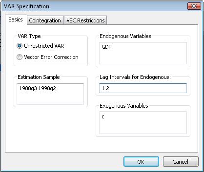
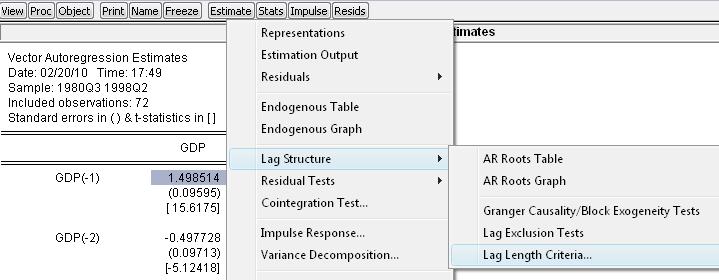
98 98

99 10.2 Lag Lengh in Muliple-Predicor Regression As in an auoregression, he SIC and AIC can be used o esimae he number of lags and he variables in he ime series regression model wih muliple predicors. Afer we deermine (and fix) he opimal lags for he auoregression, we hen coninue add successive lags of explanaory variables. If he regression model has K 99

100 coefficiens (including he inercep), he SIC and AIC are defined as: SIC(K) AIC(K) RSS(K) ln T ln K (45) T T RSS(K) 2 ln K (46) T T There are wo imporan pracical consideraions when using an informaion crierion o esimae he lag lengh. Firs, as is he case for he auoregression, all he candidae models mus be esimaed over he same sample. Second, when here are muliple predicors, his approach is compuaionally demanding because i requires many differen models. According o Sock and Wason (2007), in pracice, a convenien shorcu is o require all he regressors o have he same number of lags, ha is, o require ha p = q1 = = qk. This does, herefore, no provide he bes lag lengh srucure. 11. BOUNDS TEST FOR COINTEGRATION Anoher way o es for coinegraion and causaliy is he Bounds Tes for Coinegraion wihin ARDL modelling approach. This model was developed by Pesaran e al. (2001) and can be applied irrespecive of he order of inegraion of he variables (irrespecive of wheher regressors are purely I(0), purely I(1) or muually coinegraed). This is specially linked wih he ECM models and called VECM as specified in Secion

101 11.1 The Model The ARDL modelling approach involves esimaing he following error correcion models: Y 0y 1y Y m m 1 2yX 1 iy i jx j u1 (47) i1 j1 X 0x 1x Y m m 1 2xX 1 ix i jy j u2 (48) i1 j Tes Procedure Suppose we have Y and X are nonsaionary. Sep 1: Tesing for he uni roo of Y and X (using eiher DF, ADF, or PP ess) Suppose he es resuls indicae ha Y and X have differen orders of inegraion [I(0) and/or I(1)]. Sep 2: Tesing for coinegraion beween Y and X (using Bounds es approach) For equaions 1 and 2, he F-es (normal Wald es) is used for invesigaing one or more long-run relaionships. In he case of one or more long-run relaionships, he F-es indicaes which variable should be normalized. In equaion (47), when Y is he dependen variable, he null hypohesis of no coinegraion is H0: 1y = 2y = 0 and he alernaive hypohesis of coinegraion is H1: 1y 2y

102 On he oher hand, in equaion (48), when X is he dependen variable, he null hypohesis of no coinegraion is H0: 1x = 2x = 0 and he alernaive hypohesis of coinegraion is H1: 1x 2x 0. In his model, we sill apply he Granger causaliy es following he same procedure presened above. 12. SUGGESTED RESEARCH TOPICS From previous sudies, I would like o sugges he following opics ha you can consider for your coming research proposal. Saving, Invesmen and Economic Developmen An analysis of he ineracion among savings, invesmens and growh in Vienam Are saving and invesmen coinegraed? The case of Vienam Causal relaionship beween domesic savings and economic growh: Evidence from Vienam Does saving really maer for growh? Evidence from Vienam The relaionship beween savings and growh: Coinegraion and causaliy evidence from Vienam The saving and invesmen nexus for Vienam: Evidence from coinegraion ess 102

103 Do foreign direc invesmen and gross domesic invesmen promoe economic growh? Foreign direc invesmen and economic growh in Vienam: An empirical sudy of causaliy and error correcion mechanisms The ineracions among foreign direc invesmen, economic growh, degree of openness and unemploymen in Vienam Trade and Economic Developmen How rade and foreign invesmen affec he growh: A case of Vienam? Trade, foreign direc invesmen and economic growh in Vienam A coinegraion analysis of he long-run relaionship beween black and official foreign exchange raes: The case of he Vienam dong An empirical invesigaion of he causal relaionship beween openness and economic growh in Vienam Expor and economic growh in Vienam: A Granger causaliy analysis Expor expansion and economic growh: Tesing for coinegraion and causaliy for Vienam Is he expor-led growh hypohesis valid for Vienam? Is here a long-run relaionship beween expors and impors in Vienam? 103

104 On economic growh, FDI and expors in Vienam Trade liberalizaion and indusrial growh in Vienam: A coinegraion analysis Sock Marke and Economic Developmen Causaliy beween financial developmen and economic growh: An applicaion of vecor error correcion o Vienam Financial developmen and he FDI growh nexus: The Vienam case Macroeconomic environmen and sock marke: The Vienam case The relaionship beween economic facors and equiy marke in Vienam Modelling he linkages beween he US and Vienam sock markes The long-run relaionship beween sock reurns and inflaion in Vienam The relaionship beween financial deepening and economic growh in Vienam Tesing marke efficien hypohesis: The Vienam sock marke Threshold adjusmen in he long-run relaionship beween sock prices and economic aciviy 104

105 Energy and he Economy The dynamic relaionship beween he GDP, impors and domesic producion of crude oil: Evidence from Vienam Causal relaionship beween gas consumpion and economic growh: A case of Vienam Causal relaionship beween energy consumpion and economic growh: The case of Vienam Causaliy relaionship beween elecriciy consumpion and GDP in Vienam The causal relaionship beween elecriciy consumpion and economic growh in Vienam A coinegraion analysis of gasoline demand in Vienam Coinegraion and causaliy esing of he energy-gdp relaionship: A case of Vienam Does more energy consumpion bolser economic growh? Energy consumpion and economic growh in Vienam: Evidence from a coinegraion and error correcion model The causaliy beween energy consumpion and economic growh in Vienam The relaionship beween he price of oil and macroeconomic performance: Empirical evidence for Vienam 105

106 Fiscal Policy and Economic Developmen A causal relaionship beween governmen spending and economic developmen: An empirical examinaion of he Vienam economy Economic growh and governmen expendiure: Evidence from Vienam Governmen revenue, governmen expendiure, and emporal causaliy: Evidence from Vienam The relaionship beween budge deficis and money demand: Evidence from Vienam Moneary Policy and Economic Developmen Granger causaliy beween money and income for he Vienam economy Money, inflaion and casualiy: Evidence from Vienam Money-oupu Granger causaliy: An empirical analysis for Vienam Time-varying parameer error correcion models: The demand for money in Vienam Moneary ransmission mechanism in Vienam: A VAR analysis Tourism and Economic Developmen Coinegraion analysis of quarerly ourism demand by inernaional ouriss: Evidence from Vienam 106

107 Does ourism influence economic growh? A dynamic panel daa approach Inernaional ourism and economic developmen in Vienam: A Granger causaliy es Tourism demand modelling: Some issues regarding uni roos, co-inegraion and diagnosic ess Tourism, rade and growh: he case of Vienam Agriculure and Economic Developmen Dynamics of rice prices and agriculural wages in Vienam Macroeconomic facors and agriculural producion linkages: A case of Vienam Is agriculure he engine of growh? The causal relaionship beween ferilizer consumpion and agriculural produciviy in Vienam Macroeconomics and agriculure in Vienam Ohers Hypoheses esing concerning relaionships beween spo prices of various ypes of coffee The relaionship beween wages and prices in Vieban An error correcion model of luxury goods expendiures: Evidence from Vienam The relaionship beween macroeconomic variables and housing price index: A case of Vienam 107

108 Explaining house prices in Vienam Long-erm rend and shor-run dynamics of he Vienam gold price: an error correcion modelling approach Macroeconomic adjusmen and privae manufacuring invesmen in Vienam: A ime-series analysis Tesing for he long run relaionship beween nominal ineres raes and inflaion using coinegraion echniques The long-run relaionship beween house prices and income: Evidence from Vienam housing markes I is noed ha many empirical sudies use he nonsaionary panels, ypically characerised by panel uni roo ess and panel coinegraion ess. However, hey are beyond he scope of his lecure. 108

109 REFERENCES Aseriou, D. and Hall, S.G. (2007) Applied Economerics: A Modern Approach Using Eviews and Microfi, Revised Ediion. Palgrave Macmillan. Cheung, Y.W. and Lai, K.S. (1995) Lag Order and Criical Values of he Augmened Dickey-Fuller Tes, Journal of Business & Economic Saisics, Vol.13, No.3, pp Dickey, D.A. and Fuller, W.A. (1979) Disribuion of he Esimaors for Auoregressive Time Series wih a Uni Roo, Journal of he American Saisical Associaion, Vol.74, No.366, pp Dickey, D.A. and Fuller, W.A. (1981) Likelihood Raio Saisics for Auoregressive Time Series wih a Uni Roo, Economerica, Vol.49, p Diebold, F.X. (2004) Elemens of Forecasing, 3 rd Ediion, Thomson. Dolado, J., T.Jenkinson and S.Sosvilla-Rivero. (1990) Coinegraion and Uni Roos, Journal of Economic Surveys, Vol.4, No.3. Durbin, J. (1970) Tesing for Serial Correlaion in Leas Squares Regression When Some of he Variables Are Lagged Dependen Variables, Economerica, Vol.38, pp Engle, R.F. and Granger, C.W.J. (1987) Co-inegraion and Error Correcion Esimaes: Represenaion, Esimaion, and Tesing, Economerica, Vol.55, p

110 Granger, C.W.J. (1981) Some Properies of Time Series Daa and Their Use in Economeric Model Specificaion, Journal of Economerics, Vol.16, pp Granger, C.W.J. (1988) Some Recen Developmens in he Concep of Causaliy, Journal of Economerics, Vol.39, pp Granger, C.W.J. (2004) Time Series Analysis, Coinegraion, and Applicaions, The American Economic Review, Vol.94, No.3, pp Granger, C.W.J. and Newbold, P. (1977) Spurious Regression in Economerics, Journal of Economerics, Vol.2, pp Griffihs, W.E., R.C.Hill and G.C.Lim. (2008) Using Eviews for Principles of Economerics, 3 rd Ediion, John Wiley & Sons. Gujarai, D.N. (2003) Basic Economerics, 4 h Ediion, McGraw-Hill. Gujarai, D.N. (2011) Economerics by Example, 1 s Ediion, Palgrave Macmillan. Hanke, J.E. and Wichern, D.W. (2005) Business Forecasing, 8 h Ediion, Pearson Educaion. Holon, W.J. and Keaing, B. (2007) Business Forecasing Wih Accompanying Excel-Based ForecasXTM Sofware, 5 h Ediion, McGraw-Hill. Johansen, S. (1991) Esimaion and Hypohesis Tesing of Coinegraion Vecors in Gaussian Vecor Auoregressive Models, Economerica, Vol.59, pp Johansen, S. and Juselius, K. (1990) Maximum Likelihood Esimaion and Inference on Coinegraion, wih 110

111 Applicaions for he Demand for Money, Oxford Bullein of Economics and Saisics, Vol.52, pp Kang, H. (1985) The Effecs of Derending in Granger Causaliy Tess, Journal of Business & Economic Saisics, Vol.3, No.4, pp Kaircioglu, S. (2009) Tourism, Trade and Growh: The Case of Cyprus, Applied Economics, Vol.41, pp Li, X. (2001) Governmen Revenue, Governmen Expendiure, and Temporal Causaliy: Evidence from China, Applied Economics, Vol.33, pp Ljung, G.M. and Box, G.E.P. (1978) On a measure of Lack of Fi in Times Series Models, Biomerica, Vol.65, pp Mackinnon, J.G. (1994) Approximae Asympoic Disribuion Funcions for Uni-Roo and Coinegraion, Journal of Business & Economic Saisics, Vol.12, No.2, pp Mackinnon, J.G. (1996) Numerical Disribuion Funcions for Uni Roo and Coinegraion Tess, Journal of Applied Economerics, Vol.11, No.6, pp Mackinnon, J.G., Alfred A. Haug and Leo Michelis. (1999) Numerical Disribuion Funcions of Likelihood Raio Tess for Coinegraion, Journal of Applied Economerics, Vol.14, No.5, pp Mahmoud, E. (1984) Accuracy in Forecasing: A Survey, Journal of Forecasing, Vol.3, pp McNees, S. (1986) Forecasing Accuracy of Alernaive Techniques: A Comparison of US Macroeconomic 111

112 Forecass, Journal of Business and Economic Saisics, Vol.4, pp Mehrara, M. (2007) Energy-GDP Relaionship for Oil- Exporing Counries: Iran, Kuwai and Saudi Arabia, OPEC Review, Vol.3. Nguyen Trong Hoai, Phung Thanh Binh, and Nguyen Khanh Duy. (2009) Forecasing and Daa Analysis in Economics and Finance, Saisical Publishing House. Phillips, P.C.B. (1987) Time Series Regression wih a Uni Roo, Economerica, Vol.55, No.2, pp Phillips, P.C.B. (1998) New Tools for Undersanding Spurious Regressions, Economerica, Vol.66, No.6, pp Phillips, P.C.B. and Perron, P. (1988) Tesing for a Uni Roo in Time Series Regression, Biomerica, Vol.75, No.2, pp Pindyck, R.S. and Rubinfeld, D.L. (1998) Economeric Models and Economic Forecass, 4 h Ediion, McGraw-Hill. Ramanahan, R. (2002) Inroducory Economerics wih Applicaions, 5 h ediion, Harcour College Publisher. Sims, C.A. (1980) Macroeconomics and Realiy, Economerica, Vol.48, No.1, pp Sock, J.H. and Wason, M.W. (2007) Inroducion o Economerics, 2 nd Ediion, Pearson Educaion. Sudenmund, A.H. (2001) Using Economerics: A Pracical Guide, 4 h Ediion, Addison Wesley Longman. Toda, H.Y. and Yamamoo, T. (1995) Saisical Inference in Vecor Auoregressive wih Possibly Inegraed 112

113 Processes, Journal of Economerics, Vol.66, No.1, pp Vogelvang, B. (2005) Economerics: Theory and Applicaions wih Eviews, Pearson Educaion. Wooldridge, J.M. (2003) Inroducory Economerics: A Modern Approach, 2 nd Ediion, Thomson. 113

114 APPENDIX STATA COMMANDS Source: Pracical exercises, Advanced Economerics course 2012, Wageningen Universiy, The Neherlands. EXAMPLE 1 Use he daa se WHEATOIL.da, which conains (nominal) prices of whea (pwh), nominal oil prices (poil) and a ime indicaor (). The daa are monhly and available for he period Jan 1990 ill December 2008 (19 years*12 monhs = 228 obs.). In his example, we will invesigae wheher here is a long-run relaionship beween whea prices and oil prices. There may be all kinds of reasons for such a relaionship: oil is an imporan inpu in ferilizer producion, is used for applying machinery, drives ransporaion coss, ec. Please declare he daa o be ime-series daa using he following command: sse 1. Creae one graph wih line plos of boh pwh and poil agains. Considering he line plo for pwh, do you hink his variable is saionary? Moivae your answer. woway (sline pwh) (sline poil, yaxis(2)) 114

115 pwh poil TOPICS IN TIME SERIES ECONOMETRICS pwh poil The graphs for boh pwh and poil indicae ha here are sochasic rends (means are no consan) and heir variances are also no consan. For he pwh, i firs increases and highly flucuaes (from observaion 1 o abou 70), followed by a declining period (from observaion abou 70 o abou 120) wih less flucuaion, hen i ends o increase and especially decline very quickly in he las monhs. Therefore, we migh say ha pwh is no saionary. 2. Use appropriae ess o find ou he orders of inegraion of boh pwh and poil? 115

116 In order o check he order of inegraion for pwh we perform he Augmened Dickey Fuller (ADF) es and he KPSS es on pwh unil finding a saionary ime series. 2.1 The pwh series. ADF es H0: The pwh series is non-saionary (he pwh series has a uni roo) As his is a monhly series, we sar wih 12 lags. In addiion, we include he rend in he es equaion. 116

117 Because he coefficiens of rend and lag 12 are no saisically significan, so we can remove hese in he es equaion. If we choose he 5% significance level, he coefficiens of lag 8 o lag 11 are no significan. Therefore, we ry he es equaion wih 7 lags. 117

118 As he absolue value of he es saisics (2.579) is smaller han he absolue value of 5% criical value (2.882), we canno rejec he null hypohesis a 5% significance level. Therefore, ADF es suggess ha pwh series is no saionary. To be sure, we apply he KPSS es (wih H0: he pwh series is saionary). 118

119 KPSS es All es saisics are greaer han he 5% criical values, so we rejec he null hypohesis. Tha means he pwh series is non-saionary. We now examine saionariy of he firs-differenced series of pwh wihou he consan erm in he es equaion because here is no rend in he original series of pwh. Here is he es resul. ADF es H0: The firs-difference of pwh is no saionary. 119

120 As he absolue value of he es saisics (4.796) is larger han he 5% criical value (1.95), we rejec he null hypohesis. Tha means he firs-differenced series of pwh is saionary. We now examine he KPSS es for his firs-differenced series. KPSS es H0: The firs-differenced series of pwh is saionary. 120

121 The KPSS es resuls indicae ha we fail o rejec he null hypohesis. In conclusion, he pwh series is inegraed of order one [I(1)]. 2.2 The poil series. We proceed in he same way as in he case of pwh. Firs I perform he ADF es and he KPSS es on he values of poil. ADF es H0: The poil series is no saionary. 121

122 Because he lag 11 and lag 12 are no significan, so we remove hem in he es equaion. 122

123 As he absolue value of he es saisics (3.37) is smaller han he 5% criical value (3.43), we canno rejec he null hypohesis. This implies ha he poil series is no saionary. To be sure, we apply he KPSS es. KPSS es H0: The poil series is saionary. All es saisics are greaer han he criical values (even a 1% significance level), so we rejec he null hypohesis. Tha means he poil series is non-saionary. We now examine saionariy of he firs-differenced series of poil wih he consan erm in he es equaion because here is rend in he original series of poil. Here is he es resul. 123

124 ADF es H0: The firs-difference of poil is no saionary. As he absolue value of he es saisics (4.166) is larger han he 5% criical value (2.882), we rejec he null hypohesis. The ADF es indicaes ha he firsdifferenced series of poil is saionary. We now confirm his by applying he KPSS es. KPSS es H0: The firs-difference of poil is saionary. 124

125 The KPSS es resuls indicae ha he firs-differenced series of poil is saionary. Therefore, he poil series is inegraed of order one [I(1)]. 3. Given your findings a quesion 2, consider wheher i is possible wheher here exiss a long-run (coinegraing) relaionship beween pwh and poil. As boh series are inegraed of order one, here could exis a long-run relaionship beween pwh and poil.we mus apply he coinegraion ess o see wheher here is really a long-run (or coinegraing) relaionship beween hem. 125

126 4. Esimae he poenial long-run relaionship wih pwh as dependen variable and poil as explanaory variable. Does his regression have he ypical characerisics of a spurious regression or as a coinegraing relaionship. The OLS esimaion resuls seem o be spurious because of he following signals: The -raio is very high, while he Durbin-Wason es saisic is very small (0.103). The graph of residuals from his regression (see below) show ha he residuals seem o be non-saionary. The R 2 is low (0.213); his is no really a phenomenon of spurious regression. This can be a signal of posiive auocorrelaion. To be sure, we mus apply he saisical ess. 126

127 -50 0 Residuals TOPICS IN TIME SERIES ECONOMETRICS Invesigae wheher pwh and poil are coinegraed using wo differen ess. Wha do you conclude? How do you judge he esimaion resuls of quesion 4: as a spurious regression or as a coinegraion relaionship. We will apply wo differen ess: (i) residual-based es for no coinegraion; and (ii) CRDW es for no coinegraion. Boh ess check for he coinegraion beween poil and pwh. poil and pwh are coinegraed if he residuals of he above esimaed model ( are saionary process. 127

128 5.1 Residual-based es for no coinegraion (Engle- Granger approach) Firs es: Dickey Fuller es on he residuals Null Hypohesis: he residuals are no saionary (no coinegraion) As coefficiens of rend and lag 12 are no significan, so we remove hem from he es equaion. 128

129 The es resuls indicae ha he residuals seem o be no saionary a 5% significance level. However, he consan in his es equaion is no significan, so we ry o remove i from he es equaion. 129

130 The es equaion wihou he consan erm shows ha he residuals become saionary even a 1% significance level. This confused resuls migh be due o he less power of es of he ADF es. To avoid his, we now apply he KPSS es. 130

131 The KPSS es resuls we rejec he null hypohesis ha he residuals are saionary. Therefore, here seems o be no-coinegraion beween pwh and poil. 131

132 5.2 CRDW es for no coinegraion The Durbin-Wason es saisic is 0.103, which is smaller han he 5% criical value CRDW ess for no coinegraion (~ 0.2, abou 200 observaions, 2 variables, Table 9.3, Verbeek, 2012). Therefore, we fail o rejec he null hypohesis ha he residuals is nonsaionary. In oher words, pwh and poil are no coinegraed. In conclusion, here is no long-run relaionship beween pwh and poil. Therefore, he OLS esimaion regression beween pwh and poil is likely o be spurious regression. 5. Based on your findings a he previous quesions, esimae a simple VAR or VECM (his choice depends upon finding a quesion 5). Specify only one lag. Based on his esimaed model indicae how pwh and poil relae. 132

133 Because pwh and poil are no coinegraed, so we canno apply he VECM model. I is jus possible o use he VAR model for he firs-differenced series of pwh and poil. The VAR model resuls indicae ha he p-values of coefficiens of he variable poilld. in he firs equaion (0.202) and of he variable pwhld in he second equaion (0.97) are very high. These sugges ha neiher 133

134 poil affecs pwh, nor pwh affecs poil. However, he cofficiens of pwhld in he firs equaion, and poilld. in he second equaion are highly significan. These indicae ha he firs-differenced series follow he AR process. EXAMPLE 2 In his example, we analyse he daase TEXASHOUSING.da wih monhly housing prices in four major ciies in Texas (USA): Ausin, Dallas, Houson and San Anonio. Naural logarihms of housing prices are available from January 1990 ill December 2003 (168 observaions). I is expeced ha here are regional linkages beween hese housing markes. If houses ge very expensive in one ciy, people may decide o move o anoher ciy, creaing upward pressure on housing prices in our ciies. In oher words i is assumed ha here exis a long-run (spaial) equilibrium beween hese four housing prices series. Tha is wha we will invesigae here. 1. Invesigae for all four prices series he order of inegraion. We only repor he Augmen Dickey Fuller es and KPSS es of he las sep. We recall ha: Null hypohesis in Augmened Dickey Fuller es: ime series is no saionary Null Hypohesis in KPSS es: he ime series is saionary 134

135 AUSTIN As he absolue value of he es saisics (1.554) is smaller han he 5% criical value (2.886), we canno rejec he null hypohesis. The ime series is no saionary. 135

136 136

137 The ADF es resuls indicae ha housing price in Ausin is non-saionary. However, he KPSS es indicaes he non-saionariy (a 5% significance level) up o 5 lags only. When rying o use KPSS es wihou rend, he KPSS resuls urn ou o provide a srong evidence of non-saionariy. We now es he saionariy of he firs-difference of he housing price in Ausin. As he absolue value of he es saisics (10.964) is larger han he 5% criical value (2.886), we rejec he null hypohesis. The ime series of firs differences is saionary. 137

138 Boh ADF and KPSS ess indicae ha he firsdifferenced daa of housing price in Ausin is saionary. Therefore, he housing price in Ausin is inegraed of order on [I(1)]. 138

139 DALLAS As he absolue value of he es saisics (1.792) is smaller han he 5% criical value (3.442), we canno rejec he null hypohesis. The ime series is no saionary. 139

140 Boh ADF and KPSS ess indicae ha he housing price in Dallas is non-saionary. We now es he saionariy of is firs-differenced daa. 140

141 As he absolue value of he es saisics (5.683) is smaller han he 5% criical value (2.886), we rejec he null hypohesis. The ime series is saionary. 141

142 Boh ADF and KPSS ess indicae ha he firsdifferenced daa of housing price in Dallas is saionary. Therefore, he housing price in Dallas is inegraed of order on [I(1)]. 142

143 HOUSTON 143

144 Boh ADF and KPSS ess indicae ha he housing price in Houson is non-saionary. We now es he saionariy of is firs-differenced daa. As he absolue value of he es saisics (8.323) is larger han he 5% criical value (2.886), we rejec he null hypohesis. The ime series of firs differences is saionary. 144

145 Boh ADF and KPSS ess indicae ha he firsdifferenced daa of housing price in Houson is saionary. Therefore, he housing price in Houson is inegraed of order on [I(1)]. 145

146 SAN ANTONIO 146

147 The ADF es resuls indicae ha housing price in San Anonio is non-saionary. However, he KPSS es 147

148 indicaes he non-saionariy (a 5% significance level) up o 5 lags only. When rying o use KPSS es wihou rend, he KPSS resuls urn ou o provide a srong evidence of non-saionariy. We now es he saionariy of he firs-difference of he housing price in San Anonio. 148

149 Boh ADF and KPSS ess indicae ha he firsdifferenced daa of housing price in San Anonio is saionary. Therefore, he housing price in San Anonio is inegraed of order on [I(1)]. In conclusion, all housing prices in hese ciies are inegraed of he same order one. Therefore, here could be coinegraing relaionships among hese housing prices. 149

150 2. For he variables ha have he same order of inegraion, use Johansen s rank and maximum eigenvalues ess o invesigae he rank of he coinegraing marix. Se he number of lags o 3. The maximum eigenvalues es can be obain a he reporing ab. Wha do you conclude from hese ess? All he variables have he same order of inegraion (1), so hey could be all coinegraed. In order o check ha we perform wo coinegraion ess (Johansen ess for coinegraion). Boh es check he rank of he coinegraing marix (marix ha conains he coefficiens of coinegraing relaionships). The number of coinegraion relaionships is equal o he rank of he marix. The number of coinegraion relaionships canno be larger han he number of variables minus one (in his case canno be larger han 3). Null hypohesis in boh es: r r0 where r is he rank of he marix of coinegraing relaionships. 150

151 In he race es I rejec he null hypohesis up o he rank of wo (es saisics 9.88 smaller han 15.41). The eigenvalues es rejecs he null hypohesis up o he rank of 2 (es saisics 9.55 smaller han 14.07). So I conclude ha he rank of he coinegraing marix is wo; This implies ha here exis wo long-run relaionships among housing prices in hese ciies. 3. Image ha all variables are I(0). Explain how his would be refleced in he oupu of Johansen s rank and maximum eigenvalues ess. If four variables were saionary a heir original daa [I(0)], he coinegraing marix would have full rank (r0 = 4). In he oupu of Johansen s rank and maximum eigenvalue ess, we should have found a rank of Esimae a VECM wih he appropriae number of coinegraing relaions (again se lag a 3). Wha are he long-run coinegraing relaionships? Why are some of he adjusmen parameers no significan for hese coinegraing relaions? 151

152 152

153 153

154 From he coinegraing equaions resuls, (based on he significance of he esimaed coefficiens) we realize ha here are wo long-run coinegraing relaionships beween/among house prices of: (i) Ausin and San Anonio; and (ii) Dallas, Houson, and San Anonio. The adjusmen parameers in he VECM model can be summarized as followed: Adj.Parameer Coef. P-value Significance D_ausin Yes No D_dallas No 154

155 Yes D_houson Yes Yes D_sa Yes No For Ausin: The adjusmen parameer of he second coinegraing relaion is no significan because Ausin is omied in his relaion (see _ce2 in coinegraing equaions). For Dallas: The adjusmen parameer of he firs coinegraing relaion is no significan because Dallas is omied in his relaion (see _ce1 in he coinegraing equaions). For Houson: Boh adjusmen parameers are highly significan because Houson exiss in boh relaions (see _ce1 and _ce2 in he coinegraing equaions). For San Anonia: The adjusmen parameer of he second coinegraing relaion is no significan (alhough i is included in boh he coinegraing equaions) because of lag selecion (maybe). Say, when we change from lag(3) o lag(4), boh adjusmen parameers become significan a 5% significance level. 155

156 vec ausin dallas houson sa, rend(consan) rank(2) lag(4) If he lags are 4, we can see ha here are wo long-run coinegraing relaionships beween/among house prices of: (i) Ausin, Houson and San Anonio; and (ii) Dallas, Houson, and San Anonio. 156