Preferences and Utility
|
|
|
- Florence Grant
- 6 years ago
- Views:
Transcription

1 Preferences and Utility
2 How can we formally describe an individual s preference for different amounts of a good? How can we represent his preference for a particular list of goods (a bundle) over another? We will examine under which conditions an individual s preference can be mathematically represented with a utility function. 2

3 Preference and Choice 3

4 Preference and Choice 4
5 Advantages: Preference-based approach: More tractable when the set of alternatives Xhas many elements. Choice-based approach: It is based on observables (actual choices) rather than on unobservables (I.P) Advanced Microeconomic Theory 5
6 Preference-Based Approach Preferences: attitudes of the decisionmaker towards a set of possible alternatives X. For any x, y X, how do you compare x and y? I prefer x to y (x y) I prefer y to x (y x) I am indifferent (x y) 6
7 Preference-Based Approach By asking: Tick one box (i.e., not refrain from answering) Tick only one box Don t add any new box in which the individual says, I love x and hate y We impose the assumption: Completeness: individuals must compare any two alternatives, even the ones they don t know. The individual is capable of comparing any pair of alternatives. We don t allow the individual to specify the intensity of his preferences. 7
8 Preference-Based Approach Completeness: For an pair of alternatives x, y X, the individual decision maker: x y, or y x, or both, i.e., x y Advanced Microeconomic Theory 8
9 Preference-Based Approach Not all binary relations satisfy Completeness. Example: Is the brother of : John Bob and Bob John if they are not brothers. Is the father of : John Bob and Bob John if the two individuals are not related. Not all pairs of alternatives are comparable according to these two relations. Advanced Microeconomic Theory 9

10 Preference-Based Approach Advanced Microeconomic Theory 10

11 Preference-Based Approach Advanced Microeconomic Theory 11

12 Preference-Based Approach Advanced Microeconomic Theory 12

13 Preference-Based Approach Advanced Microeconomic Theory 13
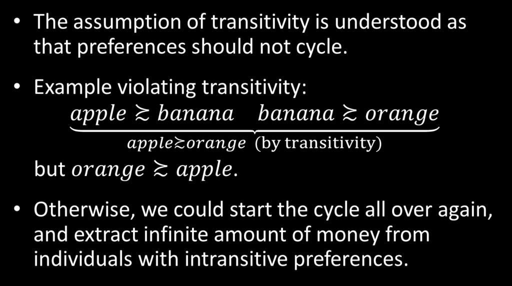
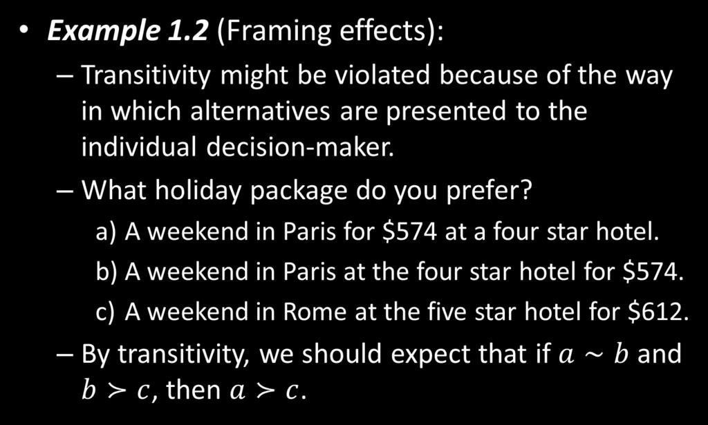
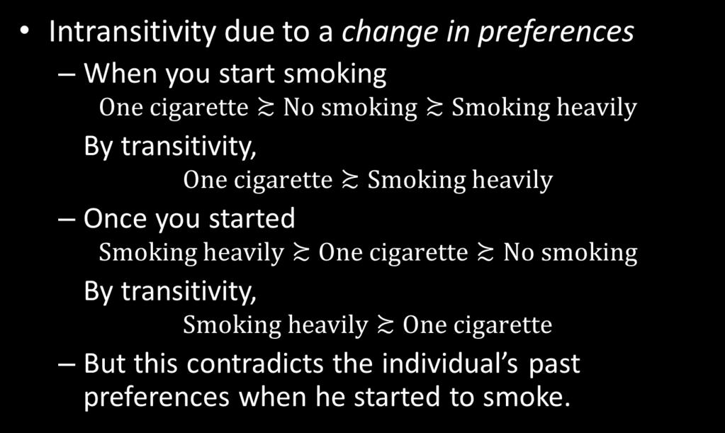
14 Preference-Based Approach Sources of intransitivity: a) Indistinguishable alternatives a) Examples? b) Framing effects c) Aggregation of criteria d) Change in preferences a) Examples? 14
15 Preference-Based Approach Example 1.1 (Indistinguishable alternatives): Take X = R as a piece of pie and x y if x y 1 (x + 1 y) but x~y if x y < 1 (indistinguishable). Then, 1.5~0.8 since = 0.7 < 1 0.8~0.3 since = 0.5 < 1 By transitivity, we would have 1.5~0.3, but in fact (intransitive preference relation). 15


16 Preference-Based Approach Other examples: similar shades of gray paint milligrams of sugar in your coffee 16
17 Preference-Based Approach 17
18 Preference-Based Approach 18
19 Preference-Based Approach 19
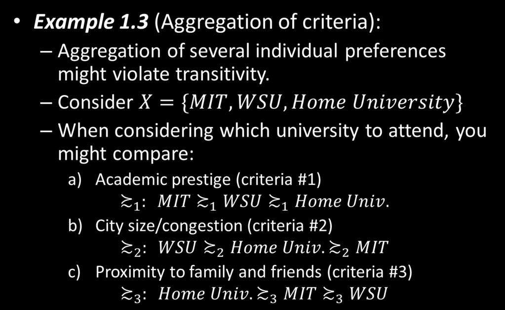
20 Preference-Based Approach Example 1.3 (continued): By majority of these considerations: MIT ณ criteria 1 & 3 WSU ณ criteria 1 & 2 Home Univ ณ criteria 2 & 3 MIT Transitivity is violated due to a cycle. A similar argument can be used for the aggregation of individual preferences in group decision-making: Every person in the group has a different (transitive) preference relation but the group preferences are not necessarily transitive ( Condorcet paradox ). 20
21 Preference-Based Approach 21

22 Utility Function 22

23 Utility Function 23

24 Utility Function 24
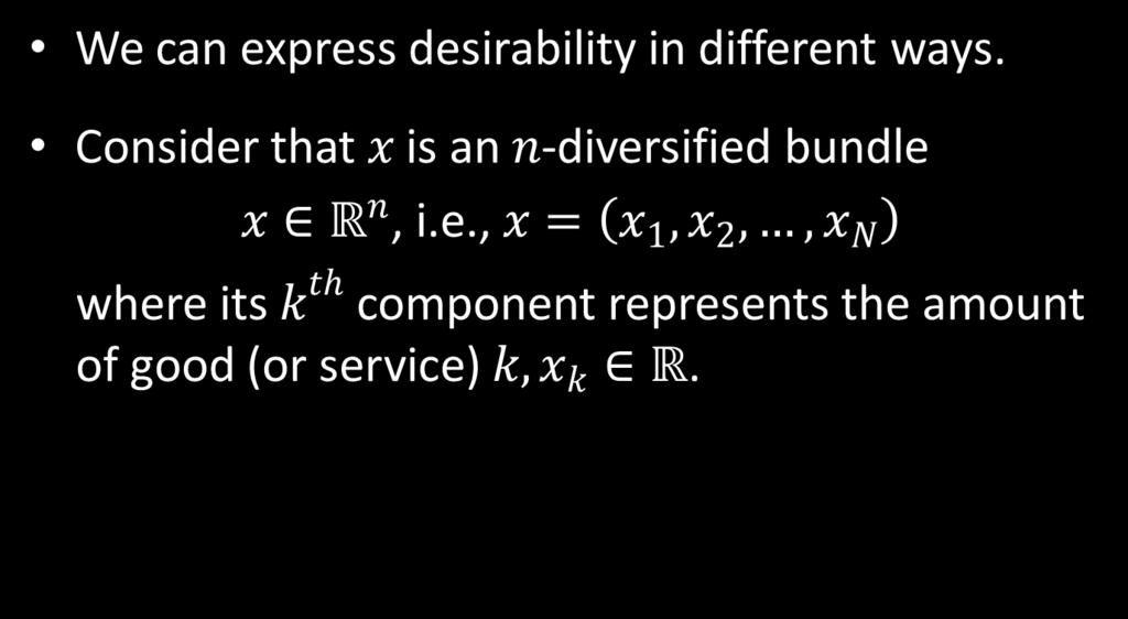
25 Desirability 25
26 Desirability 26
27 Desirability 27

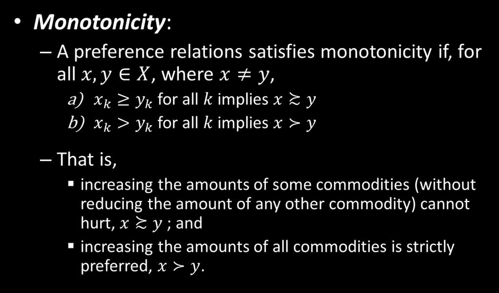
28 Desirability Advanced Microeconomic Theory 28
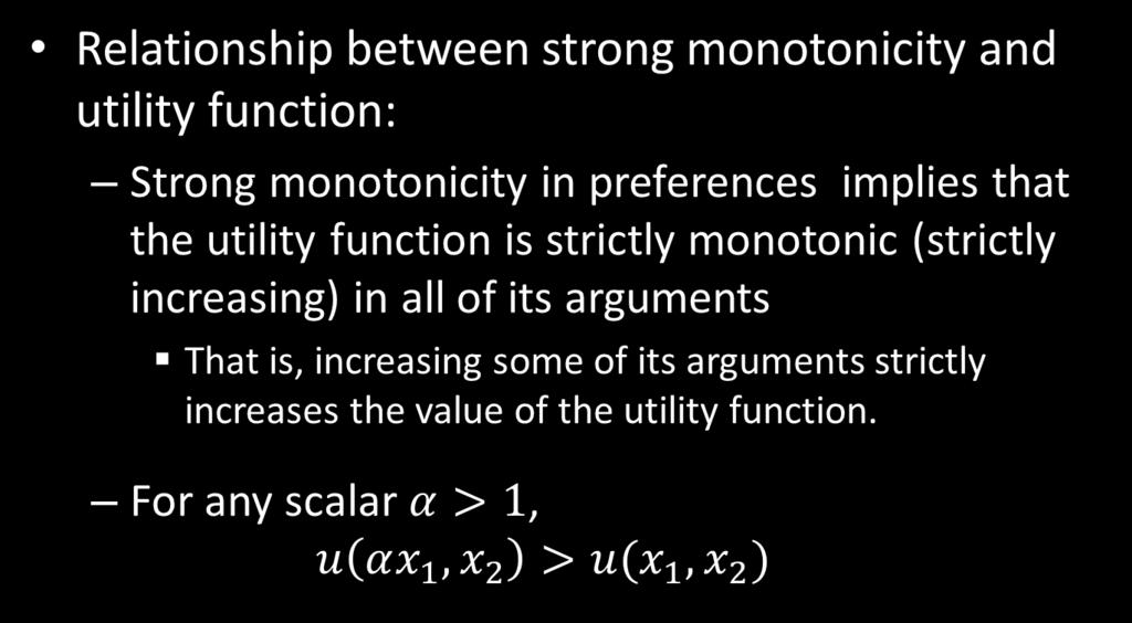
29 Desirability 29

30 Desirability Advanced Microeconomic Theory 30
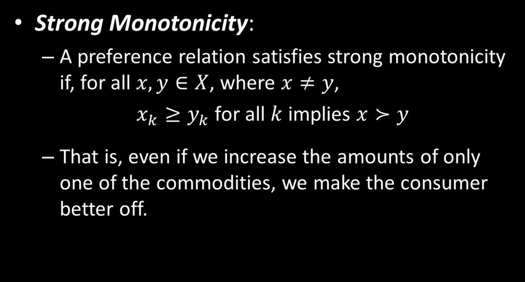
31 Desirability 31
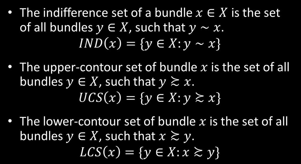
32 Indifference sets 32
33 Indifference sets x 2 x Upper contour set (UCS) {y 2 +: y x} Indifference set 2 {y +: y ~ x} Lower contour set (LCS) 2 {y +: y x} x 1 33
34 Indifference sets Note: Strong monotonicity (and monotonicity) implies that indifference curves must be negatively sloped. Hence, to maintain utility level unaffected along all the points on a given indifference curve, an increase in the amount of one good must be accompanied by a reduction in the amounts of other goods. 34

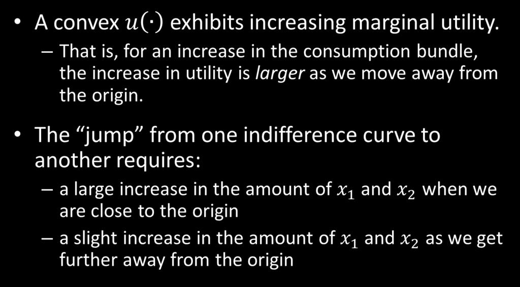
35 Convexity of Preferences 35
36 Convexity of Preferences Convexity 1 Advanced Microeconomic Theory 36

37 Convexity of Preferences 37
38 Convexity of Preferences Convexity 2 38

39 Convexity of Preferences 39
40 Convexity of Preferences Strictly convex preferences x 2 x x λx + (1 λ)y z z y y UCS x 1 40
41 Convexity of Preferences Convexity but not strict convexity λx + 1 λ y~z Such preference relation is represented by utility function such as u x 1, x 2 = ax 1 + bx 2 where x 1 and x 2 are substitutes. 41
42 Convexity of Preferences Convexity but not strict convexity λx + 1 λ y~z Such preference relation is represented by utility function such as u x 1, x 2 = min{ax 1, bx 2 } where a, b > 0. 42
43 Convexity of Preferences Example 1.6 u x 1, x 2 Satisfies convexity Satisfies strict convexity ax 1 + bx 2 X min{ax 1, bx 2 } X ax bx ax bx 2 2 X X 43
44 Convexity of Preferences Interpretation of convexity 1) Taste for diversification: An individual with convex preferences prefers the convex combination of bundles x and y, than either of those bundles alone. 44
45 Convexity of Preferences Interpretation of convexity 2) Diminishing marginal rate of substitution: MRS 1,2 u/ x 1 u/ x 2 MRS describes the additional amount of good 1 that the consumer needs to receive in order to keep her utility level unaffected. A diminishing MRS implies that the consumer needs to receive increasingly larger amounts of good 1 in order to accept further reductions of good 2. 45
46 Convexity of Preferences Diminishing marginal rate of substitution x 2 A 1 unit = x 2 B C 1 unit = x 2 D x 1 x 1 x 1 46

47 Convexity of Preferences Advanced Microeconomic Theory 47

48 Convexity of Preferences 48
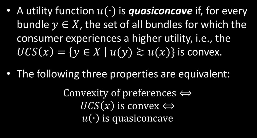
49 Quasiconcavity 49
50 Quasiconcavity 50
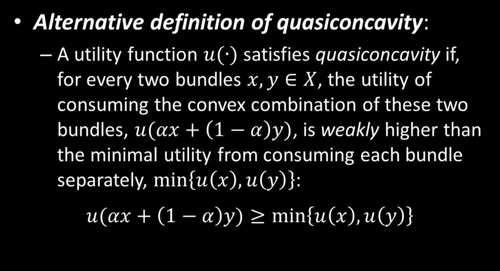
51 Quasiconcavity Quasiconcavity 51
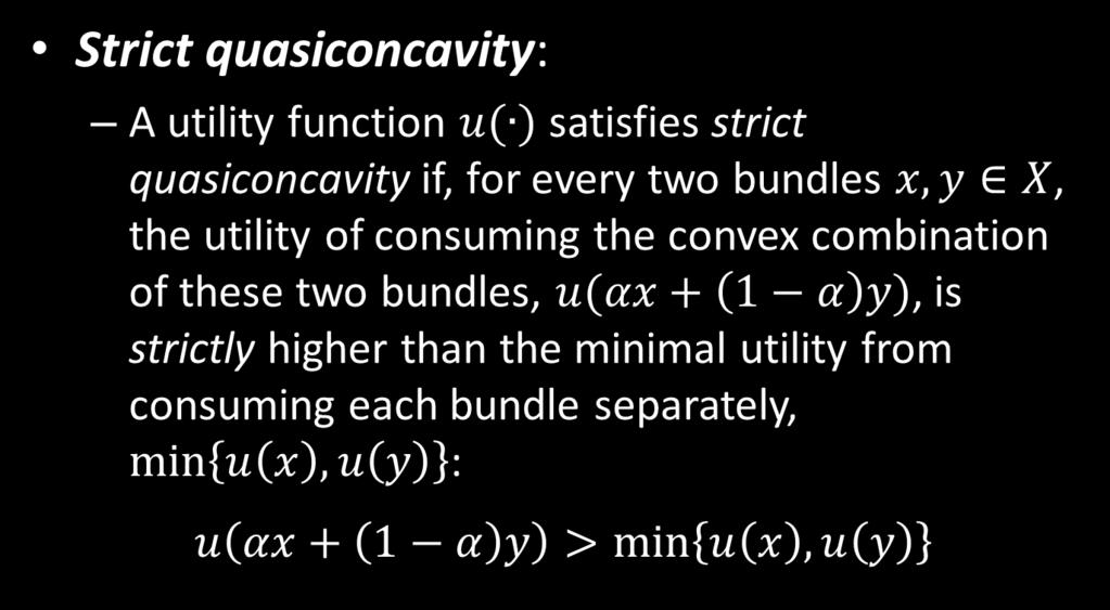
52 Quasiconcavity 52

53 Quasiconcavity x 2 x x 1 y y u x u x 1 y u y x 1 53
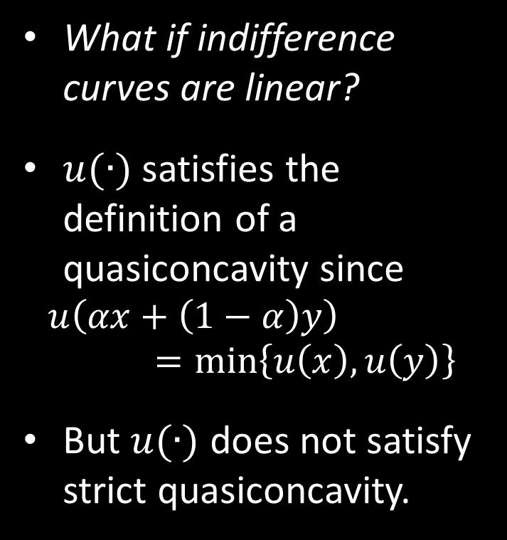
54 Quasiconcavity 54
55 Quasiconcavity 55
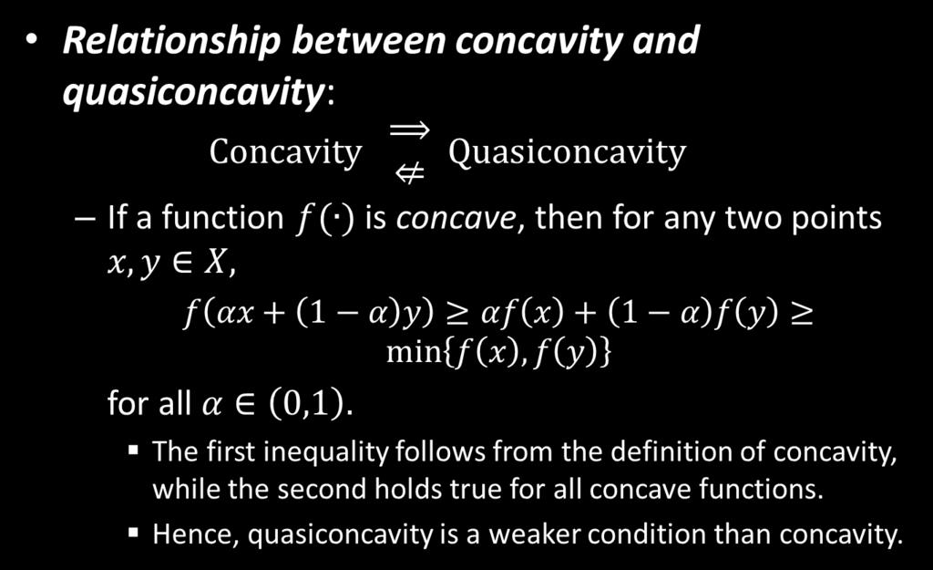
56 Quasiconcavity Concavity implies quasiconcavity 56

57 Quasiconcavity Advanced Microeconomic Theory 57
 = x 1 1 4 x 2 1 u x x x x u x 2 x 1")
58 Quasiconcavity Concave and quasiconcave utility function (3D) , u(x 1, x 2 ) = x x 2 1 u x x x x u x 2 x 1 58
59 Quasiconcavity 59
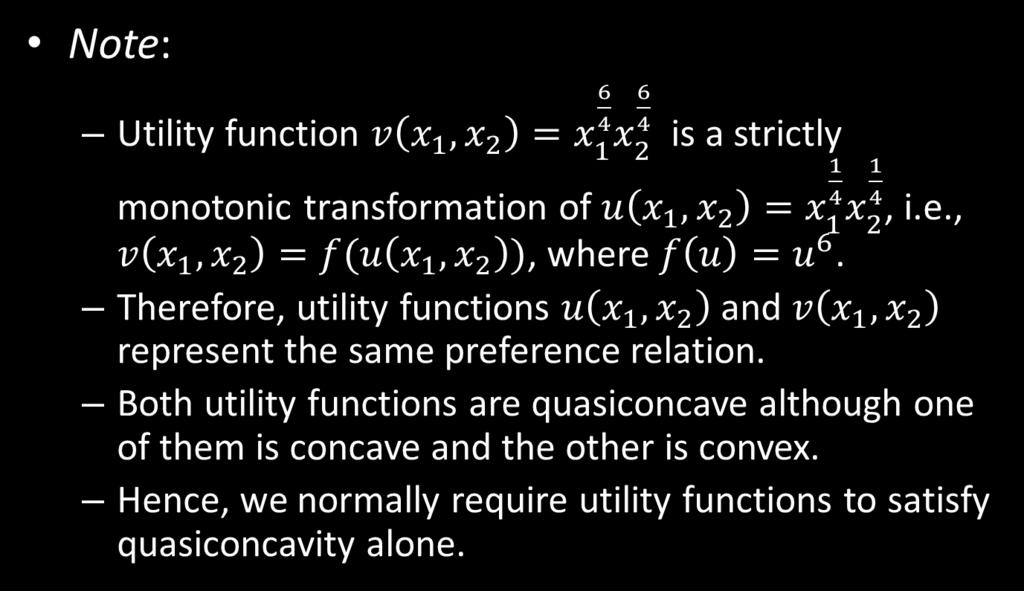
 6 6 4 1, 2 x 4 4 1 xx 1 2 v(x 1, x 2 ) = x 1 6 v x 2 x 1")
60 v x x Quasiconcavity Convex but quasiconcave utility function (3D) , 2 x xx 1 2 v(x 1, x 2 ) = x 1 6 v x 2 x 1 60
61 Quasiconcavity 61

62 Quasiconcavity Advanced Microeconomic Theory 62
63 Quasiconcavity Example 1.7 (continued): Let us consider the case of only two goods, L = 2. Then, an individual prefers a bundle x = (x 1, x 2 ) to another bundle y = (y 1, y 2 ) iff x contains more units of both goods than bundle y, i.e., x 1 y 1 and x 2 y 2. For illustration purposes, let us take bundle such as (2,1). 63
64 Quasiconcavity Example 1.7 (continued): Advanced Microeconomic Theory 64
65 Quasiconcavity Example 1.7 (continued): 1) UCS: The upper contour set of bundle (2,1) contains bundles (x 1, x 2 ) with weakly more than 2 units of good 1 and/or weakly more than 1 unit of good 2: UCS 2,1 = {(x 1, x 2 ) (2,1) x 1 2, x 2 1} The frontiers of the UCS region also represent bundles preferred to (2,1). 65
66 Quasiconcavity Example 1.7 (continued): 2) LCS: The bundles in the lower contour set of bundle (2,1) contain fewer units of both goods: LCS 2,1 = {(2,1) (x 1, x 2 ) x 1 2, x 2 1} The frontiers of the LCS region also represent bundles with fewer unis of either good 1 or good 2. 66

67 Quasiconcavity Advanced Microeconomic Theory 67
68 Quasiconcavity Example 1.7 (continued): 4) Regions A and B: Region A contains bundles with more units of good 2 but fewer units of good 1 (the opposite argument applies to region B). The consumer cannot compare bundles in either of these regions against bundle 2,1. For him to be able to rank one bundle against another, one of the bundles must contain the same or more units of all goods. 68
69 Quasiconcavity Example 1.7 (continued): 5) Preference relation is not complete: Completeness requires for every pair x and y, either x y or y x (or both). Consider two bundles x, y R + 2 with bundle x containing more units of good 1 than bundle y but fewer units of good 2, i.e., x 1 > y 1 and x 2 < y 2 (as in Region B) Then, we have neither x y nor y x. 69
70 Quasiconcavity Example 1.7 (continued): 6) Preference relation is transitive: Transitivity requires that, for any three bundles x, y and z, if x y and y z then x z. Now x y and y z means x l y l and y l z l for all l goods. Then, x l z l implies x z. 70
71 Quasiconcavity Example 1.7 (continued): 7) Preference relation is strongly monotone: Strong monotonicity requires that if we increase one of the goods in a given bundle, then the newly created bundle must be strictly preferred to the original bundle. Now x y and x y implies that x l y l for all good l and x k > y k for at least one good k. Thus, x y and x y implies x y and not y x. Thus, we can conclude that x y. 71
72 Quasiconcavity Example 1.7 (continued): 8) Preference relation is strictly convex: Strict convexity requires that if x z and y z and x z, then αx + 1 α y z for all α 0,1. Now x z and y z implies that x l y l and y l z l for all good l. x z implies, for some good k, we must have x k > z k. 72
73 Quasiconcavity Example 1.7 (continued): Hence, for any α 0,1, we must have that αx l + 1 α y l z l for all good l αx k + 1 α y k > z k for some k Thus, we have that αx + 1 α y z and αx + 1 α y z, and so αx + 1 α y z and not z αx + 1 α y Therefore, αx + 1 α y z. 73

74 Common Utility Functions 74

75 Common Utility Functions 75
76 Common Utility Functions Marginal utilities: u > 0 and u > 0 x 1 x 2 A diminishing MRS MRS x1,x 2 = αax 1 α 1 β x 2 βax α β 1 1 x = αx 2 βx 1 2 which is decreasing in x 1. Hence, indifference curves become flatter as x 1 increases. 76
77 Common Utility Functions Cobb-Douglas preference x 2 A in x 2 B x 2 C D IC 1 unit 1 unit x 1 77

78 Common Utility Functions 78
79 Common Utility Functions Perfect substitutes x 2 2A slope A B A B 2B x 1 79

80 Common Utility Functions 80

81 Common Utility Functions Advanced Microeconomic Theory 81
82 Common Utility Functions Perfect complements x 2 x x u1 u 2 2 A A 1 2 x 1 82

83 Common Utility Functions 83

84 Common Utility Functions 84
85 Common Utility Functions CES preferences x Perfect substitutes Perfect complement Cobb-Douglas x 1 Advanced Microeconomic Theory 85
86 Common Utility Functions CES utility function is often presented as u x 1, x 2 = ax 1 ρ + bx2 ρ 1 ρ where ρ σ 1 σ. 86

87 Common Utility Functions 87
88 Common Utility Functions MRS of quasilinear preferences Advanced Microeconomic Theory 88
89 Common Utility Functions For u x 1, x 2 = v x 1 + bx 2, the marginal utilities are u = b and u = v x 2 x 1 which implies MRS x1,x 2 = v x1 b x 1 Quasilinear preferences are often used to represent the consumption of goods that are relatively insensitive to income. Examples: garlic, toothpaste, etc. 89
90 Continuous Preferences In order to guarantee that preference relations can be represented by a utility function we need continuity. Continuity: A preference relation defined on X is continuous if it is preserved under limits. That is, for any sequence of pairs (x n, y n ) n=1 with x n y n for all n and lim x n = x and lim y n = y, the preference n n relation is maintained in the limiting points, i.e., x y. Advanced Microeconomic Theory 90
91 Continuous Preferences Intuitively, there can be no sudden jumps (i.e., preference reversals) in an individual preference over a sequence of bundles. Advanced Microeconomic Theory 91
92 Continuous Preferences Lexicographic preferences are not continuous Consider the sequence x n = 1 n, 0 and yn = (0,1), where n = {0,1,2,3, }. The sequence y n = (0,1) is constant in n. The sequence x n = 1 n It starts at x 1 = x 2 = 1 2, 0, x3 = 1 3, 0, etc., 0 is not: 1,0, and moves leftwards to Advanced Microeconomic Theory 92
93 Continuous Preferences Thus, the individual prefers: x 1 = 1,0 0,1 = y 1 x 2 1 y n, n, y 1 = y 2 = = y n x 2 = 1 2, 0 0,1 = y2 x 3 = 1, 0 0,1 = y3 3 But, lim n xn = 0,0 0,1 = lim n y n Preference reversal! lim x n = (0,0) n x 4 x 3 x 2 x 1 0 ⅓ ½ ¼ 1 x 1 Advanced Microeconomic Theory 93
94 Existence of Utility Function If a preference relation satisfies monotonicity and continuity, then there exists a utility function u( ) representing such preference relation. Proof: Take a bundle x 0. By monotonicity, x 0, where 0 = (0,0,, 0). That is, if bundle x 0, it contains positive amounts of at least one good and, it is preferred to bundle 0. Advanced Microeconomic Theory 94
95 Existence of Utility Function Define bundle M as the bundle where all components coincide with the highest component of bundle x: M = max {x k},, max {x k} k k Hence, by monotonicity, M x. Bundles 0 and M are both on the main diagonal, since each of them contains the same amount of good x 1 and x 2. Advanced Microeconomic Theory 95
96 Existence of Utility Function x 2 x 1 Advanced Microeconomic Theory 96
97 Existence of Utility Function By continuity and monotonicity, there exists a bundle that is indifferent to x and which lies on the main diagonal. By monotonicity, this bundle is unique Otherwise, modifying any of its components would lead to higher/lower indifference curves. Denote such bundle as t x, t x,, t(x) Let u x = t x, which is a real number. Advanced Microeconomic Theory 97
98 Existence of Utility Function Applying the same steps for another bundle y x, we obtain t y, t y,, t(y) and let u y = t y, which is also a real number. We know that x~ t x, t x,, t(x) y~ t y, t y,, t(y) x y Hence, by transitivity, x y iff x~ t x, t x,, t(x) t y, t y,, t(y) ~y Advanced Microeconomic Theory 98
99 Existence of Utility Function And by monotonicity, x y t x t y u(x) u(y) Note: A utility function can satisfy continuity but still be non-differentiable. For instance, the Leontief utility function, min{ax 1,bx 2 }, is continuous but cannot be differentiated at the kink. Advanced Microeconomic Theory 99
100 Social and Reference-Dependent Preferences We now examine social, as opposed to individual, preferences. Consider additively separable utility functions of the form u i (x i, x) = f(x i ) + g i (x) where f(x i ) captures individual i s utility from the monetary amount that he receives, x i ; g i (x) measures the utility/disutility he derives from the distribution of payoffs x = (x 1, x 2,..., x N ) among all N individuals. Advanced Microeconomic Theory 100
101 Social and Reference-Dependent Preferences Fehr and Schmidt (1999): For the case of two players, u i (x i, x j ) = x i α i max x j x i, 0 β i max x i x j, 0 where x i is player i's payoff and j i. Parameter α i represents player i s disutility from envy When x i < x j, max x j x i, 0 max x i x j, 0 = 0. Hence, u i (x i, x j ) = x i α i (x j x i ). = x j x i > 0 but Advanced Microeconomic Theory 101
102 Social and Reference-Dependent Preferences Parameter β i 0 captures player i's disutility from guilt When x i > x j, max x i x j, 0 max x j x i, 0 = 0. Hence, u i x i, x j = x i β i (x i x j ). = x i x j > 0 but Players envy is stronger than their guilt, i.e., α i β i for 0 β i < 1. Intuitively, players (weakly) suffer more from inequality directed at them than inequality directed at others. Advanced Microeconomic Theory 102
103 Social and Reference-Dependent Preferences Thus players exhibit concerns for fairness (or social preferences ) in the distribution of payoffs. If α i = β i = 0 for every player i, individuals only care about their material payoff u i (x i, x j ) = x i. Preferences coincide with the individual preferences. Advanced Microeconomic Theory 103
104 Social and Reference-Dependent Preferences Fehr and Schmidt s (1999) preferences x i 45 o -line IC 2 IC 1 x j Advanced Microeconomic Theory 104
105 Social and Reference-Dependent Preferences Bolton and Ockenfels (2000): Similar to Fehr and Schmidt (1999), but allow for non-linearities where u i ( ) u i x i, x i x i +x j increases in x i (i.e., selfish component) decreases in the share of total payoffs that individual x i enjoys, i (i.e., social preferences) x i +x j Advanced Microeconomic Theory 105
106 Social and Reference-Dependent Preferences For instance, u i x i, x i x i +x j = x i α x i x i +x j Letting u = u and solving for x j yields x j = x i α 2 u x i 2 u x i 2 which produces non-linear indifference curves. 1 2 Advanced Microeconomic Theory 106
107 Social and Reference-Dependent Preferences Andreoni and Miller (2002): A CES utility function ρ ρ u i (x i, x j ) = αx i + 1 α xj 1 ρ where x i and x j are the monetary payoff of individual i rather than the amounts of goods. If individual i is completely selfish, i.e., α = 1, u(x i ) = x i Advanced Microeconomic Theory 107
108 Social and Reference-Dependent Preferences If α (0,1), parameter ρ captures the elasticity of substitution between individual i's and j's payoffs. That is, if x j decreases by one percent, x i needs to be increased by ρ percent for individual i to maintain his utility level unaffected. Advanced Microeconomic Theory 108
109 Choice Based Approach We now focus on the actual choice behavior rather than individual preferences. From the alternatives in set A, which one would you choose? A choice structure (B, c( )) contains two elements: 1) B is a family of nonempty subsets of X, so that every element of B is a set B X. Advanced Microeconomic Theory 109
110 Choice Based Approach Example 1: In consumer theory, B is a particular set of all the affordable bundles for a consumer, given his wealth and market prices. Example 2: B is a particular list of all the universities where you were admitted, among all universities in the scope of your imagination X, i.e., B X. Advanced Microeconomic Theory 110
111 Choice Based Approach 2) c( ) is a choice rule that selects, for each budget set B, a subset of elements in B, with the interpretation that c(b) are the chosen elements from B. Example 1: In consumer theory, c(b) would be the bundles that the individual chooses to buy, among all bundles he can afford in budget set B; Example 2: In the example of the universities, c(b) would contain the university that you choose to attend. Advanced Microeconomic Theory 111
112 Choice Based Approach Note: If c(b) contains a single element, c( ) is a function; If c(b) contains more than one element, c( ) is correspondence. Advanced Microeconomic Theory 112
113 Choice Based Approach Example 1.10 (Choice structures): Define the set of alternatives as X = {x, y, z} Consider two different budget sets B 1 = {x, y} and B 2 = {x, y, z} Choice structure one (B, c 1 ( )) c 1 B 1 = c 1 x, y = {x} c 1 B 2 = c 1 x, y, z = {x} Advanced Microeconomic Theory 113
114 Choice Based Approach Example 1.10 (continued): Choice structure two (B, c 2 ( )) c 2 B 1 = c 2 x, y = {x} c 2 B 2 = c 2 x, y, z = {y} Is such a choice rule consistent? We need to impose a consistency requirement on the choice-based approach, similar to rationality assumption on the preference-based approach. Advanced Microeconomic Theory 114
115 Consistency on Choices: the Weak Axiom of Revealed Preference (WARP) Advanced Microeconomic Theory 115
116 WARP Weak Axiom of Revealed Preference (WARP): The choice structure (B, c( )) satisfies the WARP if: 1) for some budget set B B with x, y B, we have that element x is chosen, x c(b), then 2) for any other budget set B B where alternatives x and y are also available, x, y B, and where alternative y is chosen, y c(b ), then we must have that alternative x is chosen as well, x c(b ). Advanced Microeconomic Theory 116
117 WARP Example 1.11 (Checking WARP in choice structures): Take budget set B = {x, y} with the choice rule of c x, y = x. Then, for budget set B = {x, y, z}, the legal choice rules are either: c x, y, z = {x}, or c x, y, z = {z}, or c x, y, z = {x, z} Advanced Microeconomic Theory 117
118 WARP Example 1.11 (continued): This implies, individual decision-maker cannot select c x, y, z {y} c x, y, z {y, z} c x, y, z {x, y} Advanced Microeconomic Theory 118
119 WARP Example 1.12 (More on choice structures satisfying/violating WARP: Take budget set B = {x, y} with the choice rule of c x, y = {x, y}. Then, for budget set B = {x, y, z}, the legal choices according to WARP are either: c x, y, z = {x, y}, or c x, y, z = {z}, or c x, y, z = {x, y, z} Advanced Microeconomic Theory 119
120 WARP Example 1.12 (continued): Choice rule satisfying WARP B C(B) x y C(B ) B Advanced Microeconomic Theory 120
: Choice rule violating WARP B C(B) x y")
121 WARP Example 1.12 (continued): Choice rule violating WARP B C(B) x y C(B ) B Advanced Microeconomic Theory 121
122 Consumption Sets Consumption set: a subset of the commodity space R L, denoted by x R L, whose elements are the consumption bundles that the individual can conceivably consume, given the physical constrains imposed by his environment. Let us denote a commodity bundle x as a vector of L components. Advanced Microeconomic Theory 122
123 Consumption Sets Physical constraint on the labor market Advanced Microeconomic Theory 123
124 Consumption Sets Consumption at two different locations Beer in Seattle at noon x Beer in Barcelona at noon Advanced Microeconomic Theory 124
125 Consumption Sets Convex consumption sets: A consumption set X is convex if, for two consumption bundles x, x X, the bundle x = αx + 1 α x is also an element of X for any α (0,1). Intuitively, a consumption set is convex if, for any two bundles that belong to the set, we can construct a straight line connecting them that lies completely within the set. Advanced Microeconomic Theory 125
126 Consumption Sets: Economic Constraints Assumptions on the price vector in R L : 1) All commodities can be traded in a market, at prices that are publicly observable. This is the principle of completeness of markets It discards the possibility that some goods cannot be traded, such as pollution. 2) Prices are strictly positive for all L goods, i.e., p 0 for every good k. Some prices could be negative, such as pollution. Advanced Microeconomic Theory 126
127 Consumption Sets: Economic Constraints 3) Price taking assumption: a consumer s demand for all L goods represents a small fraction of the total demand for the good. Advanced Microeconomic Theory 127
128 Consumption Sets: Economic Constraints Bundle x R + L is affordable if p 1 x 1 + p 2 x p L x L w or, in vector notation, p x w. Note that p x is the total cost of buying bundle x = (x 1, x 2,, x L ) at market prices p = (p 1, p 2,, p L ), and w is the total wealth of the consumer. When x R + L then the set of feasible consumption bundles consists of the elements of the set: B p,w = {x R + L : p x w} Advanced Microeconomic Theory 128
129 Consumption Sets: Economic Constraints Example: B p,w = {x R + 2 : p 1 x 1 + p 2 x 2 w} p 1 x 1 + p 2 x 2 = w x 2 = w p 2 p 1 p 2 x 1 x 2 w p2 p - 1 (slope) p 2 2 {x +:p x = w} w p1 x 1 Advanced Microeconomic Theory 129

130 Consumption Sets: Economic Constraints Example: B p,w = {x R + 3 : p 1 x 1 + p 2 x 2 + p 3 x 3 w} Budget hyperplane x 3 x 1 x 2 Advanced Microeconomic Theory 130
131 Consumption Sets: Economic Constraints Price vector p is orthogonal to the budget line B p,w. Note that p x = w holds for any bundle x on the budget line. Take any other bundle x which also lies on B p,w. Hence, p x = w. Then, p x = p x = w p x x = 0 or p x = 0 Advanced Microeconomic Theory 131
132 Consumption Sets: Economic Constraints Since this is valid for any two bundles on the budget line, then p must be perpendicular to x on B p,w. This implies that the price vector is perpendicular (orthogonal) to B p,w. Advanced Microeconomic Theory 132
133 Consumption Sets: Economic Constraints The budget set B p,w is convex. We need that, for any two bundles x, x B p,w, their convex combination x = αx + 1 α x also belongs to the B p,w, where α (0,1). Since p x w and p x w, then p x = pαx + p 1 α x = αpx + 1 α px w Advanced Microeconomic Theory 133
Midterm #1 EconS 527 Wednesday, February 21st, 2018
 NAME: Midterm #1 EconS 527 Wednesday, February 21st, 2018 Instructions. Show all your work clearly and make sure you justify all your answers. 1. Question 1 [10 Points]. Discuss and provide examples of
Solution Homework 1 - EconS 501
 Solution Homework 1 - EconS 501 1. [Checking properties of preference relations-i]. For each of the following preference relations in the consumption of two goods (1 and 2): describe the upper contour
Chapter 1 - Preference and choice
 http://selod.ensae.net/m1 Paris School of Economics (selod@ens.fr) September 27, 2007 Notations Consider an individual (agent) facing a choice set X. Definition (Choice set, "Consumption set") X is a set
Structural Properties of Utility Functions Walrasian Demand
 Structural Properties of Utility Functions Walrasian Demand Econ 2100 Fall 2017 Lecture 4, September 7 Outline 1 Structural Properties of Utility Functions 1 Local Non Satiation 2 Convexity 3 Quasi-linearity
Preferences and Utility
 Preferences and Utility This Version: October 6, 2009 First Version: October, 2008. These lectures examine the preferences of a single agent. In Section 1 we analyse how the agent chooses among a number
Microeconomic Analysis
 Microeconomic Analysis Seminar 1 Marco Pelliccia (mp63@soas.ac.uk, Room 474) SOAS, 2014 Basics of Preference Relations Assume that our consumer chooses among L commodities and that the commodity space
Microeconomics. Joana Pais. Fall Joana Pais
 Microeconomics Fall 2016 Primitive notions There are four building blocks in any model of consumer choice. They are the consumption set, the feasible set, the preference relation, and the behavioural assumption.
Week 6: Consumer Theory Part 1 (Jehle and Reny, Chapter 1)
") Week 6: Consumer Theory Part 1 (Jehle and Reny, Chapter 1) Tsun-Feng Chiang* *School of Economics, Henan University, Kaifeng, China November 2, 2014 1 / 28 Primitive Notions 1.1 Primitive Notions Consumer
Week 6: Consumer Theory Part 1 (Jehle and Reny, Chapter 1) Tsun-Feng Chiang* *School of Economics, Henan University, Kaifeng, China November 2, 2014 1 / 28 Primitive Notions 1.1 Primitive Notions Consumer
Individual decision-making under certainty
 Individual decision-making under certainty Objects of inquiry Our study begins with individual decision-making under certainty Items of interest include: Feasible set Objective function (Feasible set R)
EconS 501 Final Exam - December 10th, 2018
 EconS 501 Final Exam - December 10th, 018 Show all your work clearly and make sure you justify all your answers. NAME 1. Consider the market for smart pencil in which only one firm (Superapiz) enjoys a
Solution Homework 1 - EconS 501
 Solution Homework 1 - EconS 501 1. [Checking properties of preference relations-i]. Moana and Maui need to find the magical fish hook. Maui lost this weapon after stealing the heart of Te Fiti and his
Week 9: Topics in Consumer Theory (Jehle and Reny, Chapter 2)
") Week 9: Topics in Consumer Theory (Jehle and Reny, Chapter 2) Tsun-Feng Chiang *School of Economics, Henan University, Kaifeng, China November 15, 2015 Microeconomic Theory Week 9: Topics in Consumer Theory
Week 9: Topics in Consumer Theory (Jehle and Reny, Chapter 2) Tsun-Feng Chiang *School of Economics, Henan University, Kaifeng, China November 15, 2015 Microeconomic Theory Week 9: Topics in Consumer Theory
Last Revised: :19: (Fri, 12 Jan 2007)(Revision:
(Revision:") 0-0 1 Demand Lecture Last Revised: 2007-01-12 16:19:03-0800 (Fri, 12 Jan 2007)(Revision: 67) a demand correspondence is a special kind of choice correspondence where the set of alternatives is X = { x
0-0 1 Demand Lecture Last Revised: 2007-01-12 16:19:03-0800 (Fri, 12 Jan 2007)(Revision: 67) a demand correspondence is a special kind of choice correspondence where the set of alternatives is X = { x
Notes I Classical Demand Theory: Review of Important Concepts
 Notes I Classical Demand Theory: Review of Important Concepts The notes for our course are based on: Mas-Colell, A., M.D. Whinston and J.R. Green (1995), Microeconomic Theory, New York and Oxford: Oxford
Revealed Preferences and Utility Functions
 Revealed Preferences and Utility Functions Lecture 2, 1 September Econ 2100 Fall 2017 Outline 1 Weak Axiom of Revealed Preference 2 Equivalence between Axioms and Rationalizable Choices. 3 An Application:
Recitation 2-09/01/2017 (Solution)
") Recitation 2-09/01/2017 (Solution) 1. Checking properties of the Cobb-Douglas utility function. Consider the utility function u(x) Y n i1 x i i ; where x denotes a vector of n di erent goods x 2 R n +,
Recitation 2-09/01/2017 (Solution) 1. Checking properties of the Cobb-Douglas utility function. Consider the utility function u(x) Y n i1 x i i ; where x denotes a vector of n di erent goods x 2 R n +,
Lecture 8: Basic convex analysis
 Lecture 8: Basic convex analysis 1 Convex sets Both convex sets and functions have general importance in economic theory, not only in optimization. Given two points x; y 2 R n and 2 [0; 1]; the weighted
Expected Utility Framework
 Expected Utility Framework Preferences We want to examine the behavior of an individual, called a player, who must choose from among a set of outcomes. Let X be the (finite) set of outcomes with common
The Ohio State University Department of Economics. Homework Set Questions and Answers
 The Ohio State University Department of Economics Econ. 805 Winter 00 Prof. James Peck Homework Set Questions and Answers. Consider the following pure exchange economy with two consumers and two goods.
Positive Theory of Equilibrium: Existence, Uniqueness, and Stability
 Chapter 7 Nathan Smooha Positive Theory of Equilibrium: Existence, Uniqueness, and Stability 7.1 Introduction Brouwer s Fixed Point Theorem. Let X be a non-empty, compact, and convex subset of R m. If
i) This is simply an application of Berge s Maximum Theorem, but it is actually not too difficult to prove the result directly.
 This is simply an application of Berge s Maximum Theorem, but it is actually not too difficult to prove the result directly.") Bocconi University PhD in Economics - Microeconomics I Prof. M. Messner Problem Set 3 - Solution Problem 1: i) This is simply an application of Berge s Maximum Theorem, but it is actually not too difficult
Bocconi University PhD in Economics - Microeconomics I Prof. M. Messner Problem Set 3 - Solution Problem 1: i) This is simply an application of Berge s Maximum Theorem, but it is actually not too difficult
Microeconomics, Block I Part 1
 Microeconomics, Block I Part 1 Piero Gottardi EUI Sept. 26, 2016 Piero Gottardi (EUI) Microeconomics, Block I Part 1 Sept. 26, 2016 1 / 53 Choice Theory Set of alternatives: X, with generic elements x,
Microeconomic Theory -1- Introduction
 Microeconomic Theory -- Introduction. Introduction. Profit maximizing firm with monopoly power 6 3. General results on maximizing with two variables 8 4. Model of a private ownership economy 5. Consumer
Notes on Consumer Theory
 Notes on Consumer Theory Alejandro Saporiti Alejandro Saporiti (Copyright) Consumer Theory 1 / 65 Consumer theory Reference: Jehle and Reny, Advanced Microeconomic Theory, 3rd ed., Pearson 2011: Ch. 1.
CONSUMER DEMAND. Consumer Demand
 CONSUMER DEMAND KENNETH R. DRIESSEL Consumer Demand The most basic unit in microeconomics is the consumer. In this section we discuss the consumer optimization problem: The consumer has limited wealth
Consumer theory Topics in consumer theory. Microeconomics. Joana Pais. Fall Joana Pais
 Microeconomics Fall 2016 Indirect utility and expenditure Properties of consumer demand The indirect utility function The relationship among prices, incomes, and the maximised value of utility can be summarised
Economics 101. Lecture 2 - The Walrasian Model and Consumer Choice
 Economics 101 Lecture 2 - The Walrasian Model and Consumer Choice 1 Uncle Léon The canonical model of exchange in economics is sometimes referred to as the Walrasian Model, after the early economist Léon
Microeconomics II. MOSEC, LUISS Guido Carli Problem Set n 3
 Microeconomics II MOSEC, LUISS Guido Carli Problem Set n 3 Problem 1 Consider an economy 1 1, with one firm (or technology and one consumer (firm owner, as in the textbook (MWG section 15.C. The set of
Mathematical Economics: Lecture 16
 Mathematical Economics: Lecture 16 Yu Ren WISE, Xiamen University November 26, 2012 Outline 1 Chapter 21: Concave and Quasiconcave Functions New Section Chapter 21: Concave and Quasiconcave Functions Concave
Lecture 3 - Axioms of Consumer Preference and the Theory of Choice
 Lecture 3 - Axioms of Consumer Preference and the Theory of Choice David Autor 14.03 Fall 2004 Agenda: 1. Consumer preference theory (a) Notion of utility function (b) Axioms of consumer preference (c)
Utility Maximization Problem
 Demand Theory Utility Maximization Problem Consumer maximizes his utility level by selecting a bundle x (where x can be a vector) subject to his budget constraint: max x 0 u(x) s. t. p x w Weierstrass
Week 7: The Consumer (Malinvaud, Chapter 2 and 4) / Consumer November Theory 1, 2015 (Jehle and 1 / Reny, 32
 / Consumer November Theory 1, 2015 (Jehle and 1 / Reny, 32") Week 7: The Consumer (Malinvaud, Chapter 2 and 4) / Consumer Theory (Jehle and Reny, Chapter 1) Tsun-Feng Chiang* *School of Economics, Henan University, Kaifeng, China November 1, 2015 Week 7: The Consumer
Week 7: The Consumer (Malinvaud, Chapter 2 and 4) / Consumer Theory (Jehle and Reny, Chapter 1) Tsun-Feng Chiang* *School of Economics, Henan University, Kaifeng, China November 1, 2015 Week 7: The Consumer
CHAPTER 4: HIGHER ORDER DERIVATIVES. Likewise, we may define the higher order derivatives. f(x, y, z) = xy 2 + e zx. y = 2xy.
 = xy 2 + e zx. y = 2xy.") April 15, 2009 CHAPTER 4: HIGHER ORDER DERIVATIVES In this chapter D denotes an open subset of R n. 1. Introduction Definition 1.1. Given a function f : D R we define the second partial derivatives as
April 15, 2009 CHAPTER 4: HIGHER ORDER DERIVATIVES In this chapter D denotes an open subset of R n. 1. Introduction Definition 1.1. Given a function f : D R we define the second partial derivatives as
Microeconomic Theory-I Washington State University Midterm Exam #1 - Answer key. Fall 2016
 Microeconomic Theory-I Washington State University Midterm Exam # - Answer key Fall 06. [Checking properties of preference relations]. Consider the following preference relation de ned in the positive
Econ 121b: Intermediate Microeconomics
 Econ 121b: Intermediate Microeconomics Dirk Bergemann, Spring 2011 Week of 1/8-1/14 1 Lecture 1: Introduction 1.1 What s Economics? This is an exciting time to study economics, even though may not be so
Recitation #2 (August 31st, 2018)
") Recitation #2 (August 1st, 2018) 1. [Checking properties of the Cobb-Douglas utility function.] Consider the utility function u(x) = n i=1 xα i i, where x denotes a vector of n different goods x R n +,
Recitation #2 (August 1st, 2018) 1. [Checking properties of the Cobb-Douglas utility function.] Consider the utility function u(x) = n i=1 xα i i, where x denotes a vector of n different goods x R n +,
The Fundamental Welfare Theorems
 The Fundamental Welfare Theorems The so-called Fundamental Welfare Theorems of Economics tell us about the relation between market equilibrium and Pareto efficiency. The First Welfare Theorem: Every Walrasian
Economics 501B Final Exam Fall 2017 Solutions
 Economics 501B Final Exam Fall 2017 Solutions 1. For each of the following propositions, state whether the proposition is true or false. If true, provide a proof (or at least indicate how a proof could
Intro to Economic analysis
 Intro to Economic analysis Alberto Bisin - NYU 1 Rational Choice The central gure of economics theory is the individual decision-maker (DM). The typical example of a DM is the consumer. We shall assume
where u is the decision-maker s payoff function over her actions and S is the set of her feasible actions.
 Seminars on Mathematics for Economics and Finance Topic 3: Optimization - interior optima 1 Session: 11-12 Aug 2015 (Thu/Fri) 10:00am 1:00pm I. Optimization: introduction Decision-makers (e.g. consumers,
Advanced Microeconomics
 Advanced Microeconomics Ordinal preference theory Harald Wiese University of Leipzig Harald Wiese (University of Leipzig) Advanced Microeconomics 1 / 68 Part A. Basic decision and preference theory 1 Decisions
The Consumer, the Firm, and an Economy
 Andrew McLennan October 28, 2014 Economics 7250 Advanced Mathematical Techniques for Economics Second Semester 2014 Lecture 15 The Consumer, the Firm, and an Economy I. Introduction A. The material discussed
Definitions: A binary relation R on a set X is (a) reflexive if x X : xrx; (f) asymmetric if x, x X : [x Rx xr c x ]
![Definitions: A binary relation R on a set X is (a) reflexive if x X : xrx; (f) asymmetric if x, x X : [x Rx xr c x ]](/thumbs/72/67754492.jpg "Definitions: A binary relation R on a set X is (a) reflexive if x X : xrx; (f) asymmetric if x, x X : [x Rx xr c x ]") Binary Relations Definition: A binary relation between two sets X and Y (or between the elements of X and Y ) is a subset of X Y i.e., is a set of ordered pairs (x, y) X Y. If R is a relation between X
Binary Relations Definition: A binary relation between two sets X and Y (or between the elements of X and Y ) is a subset of X Y i.e., is a set of ordered pairs (x, y) X Y. If R is a relation between X
x 1 1 and p 1 1 Two points if you just talk about monotonicity (u (c) > 0).
 > 0).") . (a) (8 points) What does it mean for observations x and p... x T and p T to be rationalized by a monotone utility function? Notice that this is a one good economy. For all t, p t x t function. p t x
. (a) (8 points) What does it mean for observations x and p... x T and p T to be rationalized by a monotone utility function? Notice that this is a one good economy. For all t, p t x t function. p t x
Microeconomics II Lecture 4. Marshallian and Hicksian demands for goods with an endowment (Labour supply)
") Leonardo Felli 30 October, 2002 Microeconomics II Lecture 4 Marshallian and Hicksian demands for goods with an endowment (Labour supply) Define M = m + p ω to be the endowment of the consumer. The Marshallian
Leonardo Felli 30 October, 2002 Microeconomics II Lecture 4 Marshallian and Hicksian demands for goods with an endowment (Labour supply) Define M = m + p ω to be the endowment of the consumer. The Marshallian
Notes on General Equilibrium
 Notes on General Equilibrium Alejandro Saporiti Alejandro Saporiti (Copyright) General Equilibrium 1 / 42 General equilibrium Reference: Jehle and Reny, Advanced Microeconomic Theory, 3rd ed., Pearson
Public Goods and Private Goods
 Chapter 2 Public Goods and Private Goods One Public Good, One Private Good Claude and Dorothy are roommates, also. 1 They are not interested in card games or the temperature of their room. Each of them
Utility Maximization Problem. Advanced Microeconomic Theory 2
 Demand Theory Utility Maximization Problem Advanced Microeconomic Theory 2 Utility Maximization Problem Consumer maximizes his utility level by selecting a bundle x (where x can be a vector) subject to
GARP and Afriat s Theorem Production
 GARP and Afriat s Theorem Production Econ 2100 Fall 2017 Lecture 8, September 21 Outline 1 Generalized Axiom of Revealed Preferences 2 Afriat s Theorem 3 Production Sets and Production Functions 4 Profits
3/1/2016. Intermediate Microeconomics W3211. Lecture 3: Preferences and Choice. Today s Aims. The Story So Far. A Short Diversion: Proofs
 1 Intermediate Microeconomics W3211 Lecture 3: Preferences and Choice Introduction Columbia University, Spring 2016 Mark Dean: mark.dean@columbia.edu 2 The Story So Far. 3 Today s Aims 4 So far, we have
Lecture #3. General equilibrium
 Lecture #3 General equilibrium Partial equilibrium equality of demand and supply in a single market (assumption: actions in one market do not influence, or have negligible influence on other markets) General
The Walrasian Model and Walrasian Equilibrium
 The Walrasian Model and Walrasian Equilibrium 1.1 There are only two goods in the economy and there is no way to produce either good. There are n individuals, indexed by i = 1,..., n. Individual i owns
DECISIONS AND GAMES. PART I
 DECISIONS AND GAMES. PART I 1. Preference and choice 2. Demand theory 3. Uncertainty 4. Intertemporal decision making 5. Behavioral decision theory DECISIONS AND GAMES. PART II 6. Static Games of complete
Partial Differentiation
 CHAPTER 7 Partial Differentiation From the previous two chapters we know how to differentiate functions of one variable But many functions in economics depend on several variables: output depends on both
Unlinked Allocations in an Exchange Economy with One Good and One Bad
 Unlinked llocations in an Exchange Economy with One Good and One ad Chiaki Hara Faculty of Economics and Politics, University of Cambridge Institute of Economic Research, Hitotsubashi University pril 16,
Second Welfare Theorem
 Second Welfare Theorem Econ 2100 Fall 2015 Lecture 18, November 2 Outline 1 Second Welfare Theorem From Last Class We want to state a prove a theorem that says that any Pareto optimal allocation is (part
Social Choice Theory. Felix Munoz-Garcia School of Economic Sciences Washington State University. EconS Advanced Microeconomics II
 Social Choice Theory Felix Munoz-Garcia School of Economic Sciences Washington State University EconS 503 - Advanced Microeconomics II Social choice theory MWG, Chapter 21. JR, Chapter 6.2-6.5. Additional
Can everyone benefit from innovation?
 Can everyone benefit from innovation? Christopher P. Chambers and Takashi Hayashi June 16, 2017 Abstract We study a resource allocation problem with variable technologies, and ask if there is an allocation
ON BEHAVIORAL COMPLEMENTARITY AND ITS IMPLICATIONS
 ON BEHAVIORAL COMPLEMENTARITY AND ITS IMPLICATIONS CHRISTOPHER P. CHAMBERS, FEDERICO ECHENIQUE, AND ERAN SHMAYA Abstract. We study the behavioral definition of complementary goods: if the price of one
Advanced Microeconomic Theory. Chapter 6: Partial and General Equilibrium
 Advanced Microeconomic Theory Chapter 6: Partial and General Equilibrium Outline Partial Equilibrium Analysis General Equilibrium Analysis Comparative Statics Welfare Analysis Advanced Microeconomic Theory
GS/ECON 5010 section B Answers to Assignment 1 September Q1. Are the preferences described below transitive? Strictly monotonic? Convex?
 GS/ECON 5010 section B Answers to Assignment 1 September 2011 Q1. Are the preferences described below transitive? Strictly monotonic? Convex? Explain briefly. The person consumes 2 goods, food and clothing.
1 General Equilibrium
 1 General Equilibrium 1.1 Pure Exchange Economy goods, consumers agent : preferences < or utility : R + R initial endowments, R + consumption bundle, =( 1 ) R + Definition 1 An allocation, =( 1 ) is feasible
September Math Course: First Order Derivative
 September Math Course: First Order Derivative Arina Nikandrova Functions Function y = f (x), where x is either be a scalar or a vector of several variables (x,..., x n ), can be thought of as a rule which
Advanced Microeconomic Theory. Chapter 2: Demand Theory
 Advanced Microeconomic Theory Chapter 2: Demand Theory Outline Utility maximization problem (UMP) Walrasian demand and indirect utility function WARP and Walrasian demand Income and substitution effects
Choice Theory. Matthieu de Lapparent
 Choice Theory Matthieu de Lapparent matthieu.delapparent@epfl.ch Transport and Mobility Laboratory, School of Architecture, Civil and Environmental Engineering, Ecole Polytechnique Fédérale de Lausanne
Advanced Microeconomics I: Consumers, Firms and Markets Chapters 1+2
 Advanced Microeconomics I: Consumers, Firms and Markets Chapters 1+2 Prof. Dr. Oliver Gürtler Winter Term 2012/2013 1 Advanced Microeconomics I: Consumers, Firms and Markets Chapters 1+2 JJ N J 1. Introduction
Technical Results on Regular Preferences and Demand
 Division of the Humanities and Social Sciences Technical Results on Regular Preferences and Demand KC Border Revised Fall 2011; Winter 2017 Preferences For the purposes of this note, a preference relation
Advanced Microeconomics Fall Lecture Note 1 Choice-Based Approach: Price e ects, Wealth e ects and the WARP
 Prof. Olivier Bochet Room A.34 Phone 3 63 476 E-mail olivier.bochet@vwi.unibe.ch Webpage http//sta.vwi.unibe.ch/bochet Advanced Microeconomics Fall 2 Lecture Note Choice-Based Approach Price e ects, Wealth
Hicksian Demand and Expenditure Function Duality, Slutsky Equation
 Hicksian Demand and Expenditure Function Duality, Slutsky Equation Econ 2100 Fall 2017 Lecture 6, September 14 Outline 1 Applications of Envelope Theorem 2 Hicksian Demand 3 Duality 4 Connections between
Pareto Efficiency (also called Pareto Optimality)
") Pareto Efficiency (also called Pareto Optimality) 1 Definitions and notation Recall some of our definitions and notation for preference orderings. Let X be a set (the set of alternatives); we have the
Pareto Efficiency (also called Pareto Optimality) 1 Definitions and notation Recall some of our definitions and notation for preference orderings. Let X be a set (the set of alternatives); we have the
Rice University. Fall Semester Final Examination ECON501 Advanced Microeconomic Theory. Writing Period: Three Hours
 Rice University Fall Semester Final Examination 007 ECON50 Advanced Microeconomic Theory Writing Period: Three Hours Permitted Materials: English/Foreign Language Dictionaries and non-programmable calculators
Question 1. (p p) (x(p, w ) x(p, w)) 0. with strict inequality if x(p, w) x(p, w ).
 (x(p, w ) x(p, w)) 0. with strict inequality if x(p, w) x(p, w ).") University of California, Davis Date: August 24, 2017 Department of Economics Time: 5 hours Microeconomics Reading Time: 20 minutes PRELIMINARY EXAMINATION FOR THE Ph.D. DEGREE Please answer any three
University of California, Davis Date: August 24, 2017 Department of Economics Time: 5 hours Microeconomics Reading Time: 20 minutes PRELIMINARY EXAMINATION FOR THE Ph.D. DEGREE Please answer any three
General Equilibrium and Welfare
 and Welfare Lectures 2 and 3, ECON 4240 Spring 2017 University of Oslo 24.01.2017 and 31.01.2017 1/37 Outline General equilibrium: look at many markets at the same time. Here all prices determined in the
Introduction to General Equilibrium
 Introduction to General Equilibrium Juan Manuel Puerta November 6, 2009 Introduction So far we discussed markets in isolation. We studied the quantities and welfare that results under different assumptions
Introduction to General Equilibrium: Framework.
 Introduction to General Equilibrium: Framework. Economy: I consumers, i = 1,...I. J firms, j = 1,...J. L goods, l = 1,...L Initial Endowment of good l in the economy: ω l 0, l = 1,...L. Consumer i : preferences
Existence, Computation, and Applications of Equilibrium
 Existence, Computation, and Applications of Equilibrium 2.1 Art and Bart each sell ice cream cones from carts on the boardwalk in Atlantic City. Each day they independently decide where to position their
Department of Economics The Ohio State University Final Exam Questions and Answers Econ 8712
 Prof. Peck Fall 20 Department of Economics The Ohio State University Final Exam Questions and Answers Econ 872. (0 points) The following economy has two consumers, two firms, and three goods. Good is leisure/labor.
Problem Set 1 Welfare Economics
 Problem Set 1 Welfare Economics Solutions 1. Consider a pure exchange economy with two goods, h = 1,, and two consumers, i =1,, with utility functions u 1 and u respectively, and total endowment, e = (e
Mathematical Foundations -1- Constrained Optimization. Constrained Optimization. An intuitive approach 2. First Order Conditions (FOC) 7
 7") Mathematical Foundations -- Constrained Optimization Constrained Optimization An intuitive approach First Order Conditions (FOC) 7 Constraint qualifications 9 Formal statement of the FOC for a maximum
Mathematical Foundations -- Constrained Optimization Constrained Optimization An intuitive approach First Order Conditions (FOC) 7 Constraint qualifications 9 Formal statement of the FOC for a maximum
Advanced Microeconomic Analysis, Lecture 6
 Advanced Microeconomic Analysis, Lecture 6 Prof. Ronaldo CARPIO April 10, 017 Administrative Stuff Homework # is due at the end of class. I will post the solutions on the website later today. The midterm
Economics 201b Spring 2010 Solutions to Problem Set 1 John Zhu
 Economics 201b Spring 2010 Solutions to Problem Set 1 John Zhu 1a The following is a Edgeworth box characterization of the Pareto optimal, and the individually rational Pareto optimal, along with some
Risk Aversion over Incomes and Risk Aversion over Commodities. By Juan E. Martinez-Legaz and John K.-H. Quah 1
 Risk Aversion over Incomes and Risk Aversion over Commodities By Juan E. Martinez-Legaz and John K.-H. Quah 1 Abstract: This note determines the precise connection between an agent s attitude towards income
Seminars on Mathematics for Economics and Finance Topic 5: Optimization Kuhn-Tucker conditions for problems with inequality constraints 1
 Seminars on Mathematics for Economics and Finance Topic 5: Optimization Kuhn-Tucker conditions for problems with inequality constraints 1 Session: 15 Aug 2015 (Mon), 10:00am 1:00pm I. Optimization with
Psychophysical Foundations of the Cobb-Douglas Utility Function
 Psychophysical Foundations of the Cobb-Douglas Utility Function Rossella Argenziano and Itzhak Gilboa March 2017 Abstract Relying on a literal interpretation of Weber s law in psychophysics, we show that
Problem 2: ii) Completeness of implies that for any x X we have x x and thus x x. Thus x I(x).
 Completeness of implies that for any x X we have x x and thus x x. Thus x I(x).") Bocconi University PhD in Economics - Microeconomics I Prof. M. Messner Problem Set 1 - Solution Problem 1: Suppose that x y and y z but not x z. Then, z x. Together with y z this implies (by transitivity)
Bocconi University PhD in Economics - Microeconomics I Prof. M. Messner Problem Set 1 - Solution Problem 1: Suppose that x y and y z but not x z. Then, z x. Together with y z this implies (by transitivity)
Chapter 2: Preliminaries and elements of convex analysis
 Chapter 2: Preliminaries and elements of convex analysis Edoardo Amaldi DEIB Politecnico di Milano edoardo.amaldi@polimi.it Website: http://home.deib.polimi.it/amaldi/opt-14-15.shtml Academic year 2014-15
A Comprehensive Approach to Revealed Preference Theory
 A Comprehensive Approach to Revealed Preference Theory Hiroki Nishimura Efe A. Ok John K.-H. Quah July 11, 2016 Abstract We develop a version of Afriat s Theorem that is applicable to a variety of choice
Adv. Micro Theory, ECON
 Adv. Micro Theor, ECON 6-9 Assignment Answers, Fall Due: Monda, September 7 th Directions: Answer each question as completel as possible. You ma work in a group consisting of up to 3 members for each group
Almost essential: Consumption and Uncertainty Probability Distributions MICROECONOMICS
 Prerequisites Almost essential: Consumption and Uncertainty Probability Distributions RISK MICROECONOMICS Principles and Analysis Frank Cowell July 2017 1 Risk and uncertainty In dealing with uncertainty
CHAPTER 2: CONVEX SETS AND CONCAVE FUNCTIONS. W. Erwin Diewert January 31, 2008.
 1 ECONOMICS 594: LECTURE NOTES CHAPTER 2: CONVEX SETS AND CONCAVE FUNCTIONS W. Erwin Diewert January 31, 2008. 1. Introduction Many economic problems have the following structure: (i) a linear function
Preference, Choice and Utility
 Preference, Choice and Utility Eric Pacuit January 2, 205 Relations Suppose that X is a non-empty set. The set X X is the cross-product of X with itself. That is, it is the set of all pairs of elements
Exercise 1.2. Suppose R, Q are two binary relations on X. Prove that, given our notation, the following are equivalent:
 1 Binary relations Definition 1.1. R X Y is a binary relation from X to Y. We write xry if (x, y) R and not xry if (x, y) / R. When X = Y and R X X, we write R is a binary relation on X. Exercise 1.2.
Ph.D. Preliminary Examination MICROECONOMIC THEORY Applied Economics Graduate Program June 2016
 Ph.D. Preliminary Examination MICROECONOMIC THEORY Applied Economics Graduate Program June 2016 The time limit for this exam is four hours. The exam has four sections. Each section includes two questions.
Mathematical Preliminaries for Microeconomics: Exercises
 Mathematical Preliminaries for Microeconomics: Exercises Igor Letina 1 Universität Zürich Fall 2013 1 Based on exercises by Dennis Gärtner, Andreas Hefti and Nick Netzer. How to prove A B Direct proof
Cowles Foundation for Research in Economics at Yale University
 Cowles Foundation for Research in Economics at Yale University Cowles Foundation Discussion Paper No. 1904 Afriat from MaxMin John D. Geanakoplos August 2013 An author index to the working papers in the
Solutions to selected exercises from Jehle and Reny (2001): Advanced Microeconomic Theory
: Advanced Microeconomic Theory") Solutions to selected exercises from Jehle and Reny (001): Advanced Microeconomic Theory Thomas Herzfeld September 010 Contents 1 Mathematical Appendix 1.1 Chapter A1..................................
Solutions to selected exercises from Jehle and Reny (001): Advanced Microeconomic Theory Thomas Herzfeld September 010 Contents 1 Mathematical Appendix 1.1 Chapter A1..................................
Homework 3 Suggested Answers
 Homework 3 Suggested Answers Answers from Simon and Blume are on the back of the book. Answers to questions from Dixit s book: 2.1. We are to solve the following budget problem, where α, β, p, q, I are
ARE211, Fall 2005 CONTENTS. 5. Characteristics of Functions Surjective, Injective and Bijective functions. 5.2.
 ARE211, Fall 2005 LECTURE #18: THU, NOV 3, 2005 PRINT DATE: NOVEMBER 22, 2005 (COMPSTAT2) CONTENTS 5. Characteristics of Functions. 1 5.1. Surjective, Injective and Bijective functions 1 5.2. Homotheticity
ECON 5111 Mathematical Economics
 Test 1 October 1, 2010 1. Construct a truth table for the following statement: [p (p q)] q. 2. A prime number is a natural number that is divisible by 1 and itself only. Let P be the set of all prime numbers
Econ 110: Introduction to Economic Theory. 8th Class 2/7/11
 Econ 110: Introduction to Economic Theory 8th Class 2/7/11 go over problem answers from last time; no new problems today given you have your problem set to work on; we'll do some problems for these concepts