CMSC427 Parametric curves: Hermite, Catmull-Rom, Bezier

Transcription

1 CMSC427 Parametric curves: Hermite, Catmull-Rom, Bezier

2 Modeling Creating 3D objects How to construct complicated surfaces? Goal Specify objects with few control points Resulting object should be visually pleasing (smooth) Start with curves, then generalize to surfaces 2

3 Usefulness of curves Surface of revolution 3

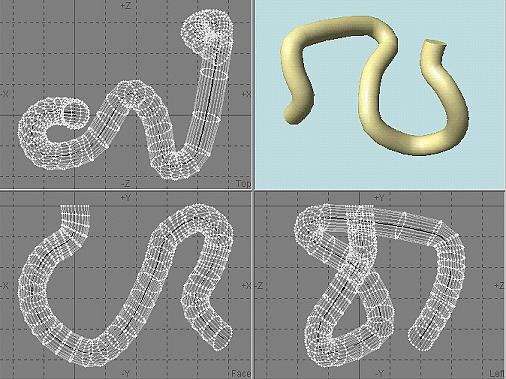
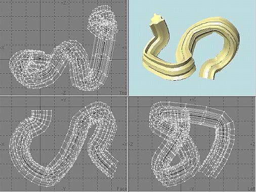
4 Usefulness of curves Extruded/swept surfaces 4

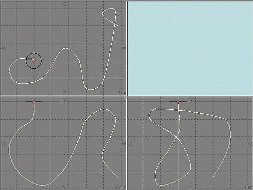
5 Usefulness of curves Animation Provide a track for objects Use as camera path 5

6 Usefulness of curves Generalize to surface patches using grids of curves, next class 6

7 How to represent curves Specify every point along curve? Hard to get precise, smooth results Too much data, too hard to work with Idea: specify curves using small numbers of control points Mathematics: use polynomials to represent curves Control point 7

8 Interpolating polynomial curves Curve goes through all control points Seems most intuitive Surprisingly, not usually the best choice Hard to predict behavior Overshoots, wiggles Hard to get nice-looking curves Control point Interpolating curve 8

9 Approximating polynomial curves Curve is influenced by control points Control point Various types & techniques based on polynomial functions Bézier curves, B-splines, NURBS Focus on Bézier curves 9

10 Mathematical definition A vector valued function of one variable x(t) Given t, compute a 3D point x=(x,y,z) May interpret as three functions x(t), y(t), z(t) Moving a point along the curve x(t) z y x(0.0) x(0.5) x(1.0) x 10

11 Tangent vector Derivative A vector that points in the direction of movement Length of x (t) corresponds to speed x(t) z y x (0.0) x (0.5) x (1.0) x 11

12 Piecewise polynomial curves Model complex shapes by sequence Use polyline to store control points 12

13 Continuity How piecewise curves join Ck continuity kth derivatives match Gk continuity kth derivatives are proportional 13

14 Hermite curves Cubic curve (here 2D) x t = at 3 + bt 6 + ct + d y t = et 3 + ft 6 + gt + h Interpolates end points P0 and P1 Matches tangent at endpoints T0 and T1 (also dp0 and dp1 in these notes). P1 = (x1,y1) T1=<dx1,dy1> P0=(x0,y0) T0=<dx0,dy0>

15 Computing coefficients a, b, c and d Derivative of x(t) x t = 3at 6 + 2bt + c Set t = 0 and 1 for endpoints Four constraints x 0 = d x (0) = c x 1 = a + b + c + d x 1 = 3a + 2b + c

16 Solve for a, b, c and d Solve for a, b, c and d d = x0 c = dx0 b = 3x0 + 3x1 2dx0 dx1 a = 2x0 2x1 + dx0 + dx1

17 Matrix version Constraints x 0 = d x (0) = c x 1 = a + b + c + d x 1 = 3a + 2b + c Give a b c d = x0 x1 dx0 dx1

18 Solve matrix version: basis matrix Since we have MA = G We can solve with A = M \] G And get Hermite basis matrix M \] a b c d = x0 x1 dx0 dx1

19 Vector version To include x, y and z, rewrite with vectors P0, P1 and tangents T0 and T1 a b c d = P0 P1 T0 T1 Coefficients a, b, c and d are now vectors

20 Full polynomial version Rewrite polynomial as dot product P t = t 3 t 6 t 1 a b c d = t 3 t 6 t P0 P1 T0 T1

21 Blending functions Instead of polynomial in t, look at curve as weighted sum of P0, P1, T0 and T1 x t = 2x0 2x1 + dx0 + dx1 t 3 + 3x0 + 3x1 2dx0 dx1 t 6 + dx0 t +x0

22 Blending functions Instead of polynomial in t, look at curve as weighted sum of P0, P1, T0 and T1 x t = 2t 3 3t x0 + 2t 3 + 3t 6 x1 + t 3 2t 6 + t dx0 + t 3 t 6 dx1

23 Blending functions h00(t) = 2t 3 3t h01(t) = 2t 3 + 3t 6 h10(t) = t 3 2t 6 + t h11(t) = t 3 t 6

24 Computing Hermite tangents Have P(-1), P0, P1 and P2 as input Compute tangent with H matrix x0 x1 dx0 dx1 = x o x ] x \] x 6

25 Combine with Hermite basis Unify notation a b c d = x o x ] x \] x 6 Final matrix a b c d = x o x ] x \] x 6

26 Catmull-Rom curves Hermite problem with C1 continuity P1 left P3 right P5 P0 P2 P4

27 Catmull-Rom curves Catmull-Rom make tangent symmetric Define by two adjacent points Here T3 = P4-P2 P1 P3 P5 P0 P2 P4

28 Catmull-Rom curves Need to change H matrix ½ traditional for C-R curves x0 x1 dx0 dx1 = /2 0 1/2 0 1/ /2 x o x ] x \] x 6

29 Catmull-Rom curves Which gives a b c d = /2 0 1/2 0 1/ /2 x o x ] x \] x 6 Or a b c d = x o x ] x \] x 6

30 Bézier curves A particularly intuitive way to define control points for polynomial curves Developed for CAD (computer aided design) and manufacturing Before games, before movies, CAD was the big application for CG Pierre Bézier (1962), design of auto bodies for Peugeot, Paul de Casteljau (1959), for Citroen 30

31 Bézier curves Higher order extension of linear interpolation Control points p 0, p 1,... p 1 p 1 p 2 p 1 p 3 p 0 p 0 p 0 p 2 Linear Quadratic Cubic 31

32 Bézier curves Intuitive control over curve given control points Endpoints are interpolated, intermediate points are approximated Convex Hull property Variation-diminishing property 32

33 Cubic Bézier curve Cubic polynomials, most common case Defined by 4 control points Two interpolated endpoints Two midpoints control the tangent at the endpoints p 1 x(t) p 0 p 2 Control polyline p 3 33

34 Bézier Curve formulation Three alternatives, analogous to linear case 1. Weighted average of control points 2. Cubic polynomial function of t 3. Matrix form Algorithmic construction de Casteljau algorithm 34

35 de Casteljau Algorithm A recursive series of linear interpolations Works for any order, not only cubic Not terribly efficient to evaluate Other forms more commonly used Why study it? Intuition about the geometry Useful for subdivision (later today) 35

36 de Casteljau Algorithm Given the control points A value of t Here t 0.25 p 1 p 0 p 2 p 3 36

37 de Casteljau Algorithm p 1 q 1 q 0 (t) = Lerp( t,p 0,p ) 1 p 0 q 0 q 1 (t) = Lerp( t,p 1,p ) 2 p 2 q 2 (t) = Lerp( t,p 2,p ) 3 q 2 p 3 37

38 de Casteljau Algorithm q 0 r 0 q 1 r 0 (t) = Lerp( t,q 0 (t),q 1 (t)) r 1 (t) = Lerp( t,q 1 (t),q 2 (t)) r 1 q 2 38

39 de Casteljau Algorithm r 0 x r 1 x(t) = Lerp( t,r 0 (t),r 1 (t)) 39

40 de Casteljau algorithm p 1 p 0 x p 2 Applets p 3 40

41 de Casteljau Algorithm Linear Quadratic Cubic Quartic 41

42 Recursive linear interpolation x = Lerp t,r 0,r 1 r = Lerp ( t,q,q ) r 1 = Lerp t,q 1,q 2 q 0 = Lerp( t,p 0,p ) 1 q 1 = Lerp( t,p 1,p ) 2 q 2 = Lerp( t,p 2,p ) 3 p 0 p 1 p 2 p 3 p 1 q 0 r 0 p 2 x q 1 r 1 p 3 q 2 p 4 42

43 Recursive linear interpolation x = Lerp t,r 0,r 1 r = Lerp ( t,q,q ) r 1 = Lerp t,q 1,q 2 q 0 = Lerp( t,p 0,p ) 1 q 1 = Lerp( t,p 1,p ) 2 q 2 = Lerp( t,p 2,p ) 3 p 0 p 1 p 2 p 3 p 1 q 0 r 0 p 2 x q 1 r 1 p 3 q 2 p 4 43

44 Recursive linear interpolation x = Lerp t,r 0,r 1 r = Lerp ( t,q,q ) r 1 = Lerp t,q 1,q 2 q 0 = Lerp( t,p 0,p ) 1 q 1 = Lerp( t,p 1,p ) 2 q 2 = Lerp( t,p 2,p ) 3 p 0 p 1 p 2 p 3 p 1 q 0 r 0 p 2 x q 1 r 1 p 3 q 2 p 4 44

45 Recursive linear interpolation x = Lerp t,r 0,r 1 r = Lerp ( t,q,q ) r 1 = Lerp t,q 1,q 2 q 0 = Lerp( t,p 0,p ) 1 q 1 = Lerp( t,p 1,p ) 2 q 2 = Lerp( t,p 2,p ) 3 p 0 p 1 p 2 p 3 p 1 q 0 r 0 p 2 x q 1 r 1 p 3 q 2 p 4 45

46 Expand the LERPs q 0 (t) = Lerp( t,p 0,p 1 )= ( 1- t)p 0 + tp 1 q 1 (t) = Lerp( t,p 1,p 2 )= ( 1- t)p 1 + tp 2 q 2 (t) = Lerp( t,p 2,p 3 )= ( 1- t)p 2 + tp 3 r 0 (t) = Lerp( t,q 0 (t),q 1 (t))= 1- t r 1 (t) = Lerp( t,q 1 (t),q 2 (t))= 1- t p 0 + tp 1 )+ t ( 1- t)p 1 + tp 2 p 1 + tp 2 )+ t ( 1- t)p 2 + tp 3 1- t 1- t x(t) = Lerp t,r 0 (t),r 1 (t) = ( 1- t) ( 1- t) ( 1- t)p 0 + tp 1 )+ t ( 1- t)p 1 + tp 2 +t ( 1- t) ( 1- t)p 1 + tp 2 )+ t ( 1- t)p 2 + tp 3 46

47 Expand the LERPs q 0 (t) = Lerp( t,p 0,p 1 )= ( 1- t)p 0 + tp 1 q 1 (t) = Lerp( t,p 1,p 2 )= ( 1- t)p 1 + tp 2 q 2 (t) = Lerp( t,p 2,p 3 )= ( 1- t)p 2 + tp 3 r 0 (t) = Lerp( t,q 0 (t),q 1 (t))= 1- t r 1 (t) = Lerp( t,q 1 (t),q 2 (t))= 1- t p 0 + tp 1 )+ t ( 1- t)p 1 + tp 2 p 1 + tp 2 )+ t ( 1- t)p 2 + tp 3 1- t 1- t x(t) = Lerp t,r 0 (t),r 1 (t) = ( 1- t) ( 1- t) ( 1- t)p 0 + tp 1 )+ t ( 1- t)p 1 + tp 2 +t ( 1- t) ( 1- t)p 1 + tp 2 )+ t ( 1- t)p 2 + tp 3 47

48 Expand the LERPs q 0 (t) = Lerp( t,p 0,p 1 )= ( 1- t)p 0 + tp 1 q 1 (t) = Lerp( t,p 1,p 2 )= ( 1- t)p 1 + tp 2 q 2 (t) = Lerp( t,p 2,p 3 )= ( 1- t)p 2 + tp 3 r 0 (t) = Lerp( t,q 0 (t),q 1 (t))= 1- t r 1 (t) = Lerp( t,q 1 (t),q 2 (t))= 1- t p 0 + tp 1 )+ t ( 1- t)p 1 + tp 2 p 1 + tp 2 )+ t ( 1- t)p 2 + tp 3 1- t 1- t x(t) = Lerp t,r 0 (t),r 1 (t) = ( 1- t) ( 1- t) ( 1- t)p 0 + tp 1 )+ t ( 1- t)p 1 + tp 2 +t ( 1- t) ( 1- t)p 1 + tp 2 )+ t ( 1- t)p 2 + tp 3 48

49 Expand the LERPs q 0 (t) = Lerp( t,p 0,p 1 )= ( 1- t)p 0 + tp 1 q 1 (t) = Lerp( t,p 1,p 2 )= ( 1- t)p 1 + tp 2 q 2 (t) = Lerp( t,p 2,p 3 )= ( 1- t)p 2 + tp 3 r 0 (t) = Lerp( t,q 0 (t),q 1 (t))= 1- t r 1 (t) = Lerp( t,q 1 (t),q 2 (t))= 1- t p 0 + tp 1 )+ t ( 1- t)p 1 + tp 2 p 1 + tp 2 )+ t ( 1- t)p 2 + tp 3 1- t 1- t x(t) = Lerp t,r 0 (t),r 1 (t) = ( 1- t) ( 1- t) ( 1- t)p 0 + tp 1 )+ t ( 1- t)p 1 + tp 2 +t ( 1- t) ( 1- t)p 1 + tp 2 )+ t ( 1- t)p 2 + tp 3 49

50 Expand the LERPs q 0 (t) = Lerp( t,p 0,p 1 )= ( 1- t)p 0 + tp 1 q 1 (t) = Lerp( t,p 1,p 2 )= ( 1- t)p 1 + tp 2 q 2 (t) = Lerp( t,p 2,p 3 )= ( 1- t)p 2 + tp 3 r 0 (t) = Lerp( t,q 0 (t),q 1 (t))= 1- t r 1 (t) = Lerp( t,q 1 (t),q 2 (t))= 1- t p 0 + tp 1 )+ t ( 1- t)p 1 + tp 2 p 1 + tp 2 )+ t ( 1- t)p 2 + tp 3 1- t 1- t x(t) = Lerp t,r 0 (t),r 1 (t) = ( 1- t) ( 1- t) ( 1- t)p 0 + tp 1 )+ t ( 1- t)p 1 + tp 2 +t ( 1- t) ( 1- t)p 1 + tp 2 )+ t ( 1- t)p 2 + tp 3 50

51 Weighted average of control points Regroup x(t) = 1- t p 0 + tp 1 )+ t ( 1 - t)p 1 + tp 2 p 1 + tp 2 )+ t( 1- t)p 2 + tp 3 ) ( 1- t) 1 - t +t 1 - t 1 - t x(t) = ( 1- t) 3 p 0 + 3( 1 - t) 2 tp 1 + 3( 1 - t)t 2 p 2 + t 3 p 3 B 0 (t ) B " $$$ # $$$ % 1 (t ) " $$ # $$ % x(t) = -t 3 + 3t 2-3t + 1 p 0 + 3t 3-6t 2 + 3t! + -3t 3 + 3t 2 & $ ' $ ( p 2 + t 3 ) p 3 B 2 (t ) B 3 (t ) p 1 51

52 Weighted average of control points Regroup x(t) = 1- t p 0 + tp 1 )+ t ( 1 - t)p 1 + tp 2 p 1 + tp 2 )+ t( 1- t)p 2 + tp 3 ) ( 1- t) 1 - t +t 1 - t 1 - t x(t) = ( 1- t) 3 p 0 + 3( 1 - t) 2 tp 1 + 3( 1 - t)t 2 p 2 + t 3 p 3 B 0 (t ) B " $$$ # $$$ % 1 (t ) " $$ # $$ % x(t) = -t 3 + 3t 2-3t + 1 p 0 + 3t 3-6t 2 + 3t! + -3t 3 + 3t 2 & $ ' $ ( p 2 + t 3 ) p 3 B 2 (t ) B 3 (t ) p 1 52

53 Weighted average of control points Regroup x(t) = 1- t p 0 + tp 1 )+ t ( 1 - t)p 1 + tp 2 p 1 + tp 2 )+ t( 1- t)p 2 + tp 3 ) ( 1- t) 1 - t +t 1 - t 1 - t x(t) = ( 1- t) 3 p 0 + 3( 1 - t) 2 tp 1 + 3( 1 - t)t 2 p 2 + t 3 p 3 B 0 (t ) B " $$$ # $$$ % 1 (t ) " $$ # $$ % x(t) = -t 3 + 3t 2-3t + 1 p 0 + 3t 3-6t 2 + 3t! + -3t 3 + 3t 2 & $ ' $ ( p 2 + t 3 ) p 3 B 2 (t ) B 3 (t ) p 1 Bernstein polynomials 53

54 Cubic Bernstein polynomials x(t) = B 0 ( t)p 0 + B 1 ( t)p 1 + B 2 ( t)p 2 + B 3 ( t)p 3 The cubic Bernstein polynomials : B 0 ( t)= -t 3 + 3t 2-3t + 1 B 1 ( t)= 3t 3-6t 2 + 3t B 2 ( t)= -3t 3 + 3t 2 ( t)= t 3 B 3 å B i (t) = 1 Partition of unity, at each t always add to 1 Endpoint interpolation, B 0 and B 3 go to 1 54

55 General Bernstein polynomials B 1 0 B 1 1 ( t)= -t + 1 B 2 0 ( t)= t 2-2t + 1 B 3 0 ( t)= -t 3 + 3t 2-3t + 1 ( t)= t B 2 1 ( t)= -2t 2 + 2t B 3 1 ( t)= 3t 3-6t 2 + 3t B 2 2 ( t)= t 2 B 3 2 ( t)= -3t 3 + 3t 2 B 3 3 ( t)= t 3 B i n æ ( t)= n ö è ç i ø ( 1- t)n-i t å B n i ( t) = 1 n i æ ö è ç i ø = n! i! ( n - i)! 55

56 General Bernstein polynomials B 1 0 B 1 1 ( t)= -t + 1 B 2 0 ( t)= t 2-2t + 1 B 3 0 ( t)= -t 3 + 3t 2-3t + 1 ( t)= t B 2 1 ( t)= -2t 2 + 2t B 3 1 ( t)= 3t 3-6t 2 + 3t B 2 2 ( t)= t 2 B 3 2 ( t)= -3t 3 + 3t 2 B 3 3 ( t)= t 3 B i n æ ( t)= n ö è ç i ø ( 1- t)n-i t å B n i ( t) = 1 n i æ ö è ç i ø = n! i! ( n - i)! 56

57 General Bernstein polynomials B 1 0 B 1 1 ( t)= -t + 1 B 2 0 ( t)= t 2-2t + 1 B 3 0 ( t)= -t 3 + 3t 2-3t + 1 ( t)= t B 2 1 ( t)= -2t 2 + 2t B 3 1 ( t)= 3t 3-6t 2 + 3t B 2 2 ( t)= t 2 B 3 2 ( t)= -3t 3 + 3t 2 B 3 3 ( t)= t 3 B i n æ ( t)= n ö è ç i ø ( 1- t)n-i t å B n i ( t) = 1 n i æ ö è ç i ø = n! i! ( n - i)! 57

58 General Bernstein polynomials B 1 0 B 1 1 ( t)= -t + 1 B 2 0 ( t)= t 2-2t + 1 B 3 0 ( t)= -t 3 + 3t 2-3t + 1 ( t)= t B 2 1 ( t)= -2t 2 + 2t B 3 1 ( t)= 3t 3-6t 2 + 3t B 2 2 ( t)= t 2 B 3 2 ( t)= -3t 3 + 3t 2 B 3 3 ( t)= t 3 Order n: B i n æ ( t)= n ö è ç i ø ( 1- t)n-i t å B n i ( t) = 1 n i æ ö è ç i ø = n! i! ( n - i)! Partition of unity, endpoint interpolation 58

59 General Bézier curves nth-order Bernstein polynomials form nth-order Bézier curves Bézier curves are weighted sum of control points using nth-order Bernstein polynomials Bernstein polynomials of order n: Bézier curve of order n: B i n æ ( t)= n ö è ç i ø ( 1- t)n-i t n å i=0 x( t)= B n i ( t)p i i 59

60 Bézier curve properties Convex hull property Variation diminishing property Affine invariance 60

61 Convex hull, convex combination Convex hull of a set of points Smallest polyhedral volume such that (i) all points are in it (ii) line connecting any two points in the volume lies completely inside it (or on its boundary) Convex combination of the points Weighted average of the points, where weights all between 0 and 1, sum up to 1 Any convex combination always lies within the convex hull p 1 p 3 Convex hull p 0 p 2 61

62 Convex hull property Bézier curve is a convex combination of the control points Bernstein polynomials add to 1 at each value of t Curve is always inside the convex hull of control points Makes curve predictable Allows efficient culling, intersection testing, adaptive tessellation p 1 p 3 p 0 p 2 62

63 Variation diminishing property If the curve is in a plane, this means no straight line intersects a Bézier curve more times than it intersects the curve's control polyline Curve is not more wiggly than control polyline Yellow line: 7 intersections with control polyline 3 intersections with curve 63

64 Affine invariance Two ways to transform Bézier curves 1. Transform the control points, then compute resulting point on curve 2. Compute point on curve, then transform it Either way, get the same transform point! Curve is defined via affine combination of points (convex combination is special case of an affine combination) Invariant under affine transformations Convex hull property always remains 64

65 Cubic polynomial form Start with Bernstein form: x(t) = (-t 3 + 3t 2-3t + 1)p 0 + ( 3t 3-6t 2 + 3t)p 1 + (-3t 3 + 3t 2 )p 2 + ( t 3 )p 3 Regroup into coefficients of t : x(t) = (-p 0 + 3p 1-3p 2 + p 3 )t 3 + ( 3p 0-6p 1 + 3p 2 )t 2 + (-3p 0 + 3p 1 )t + ( p 0 )1 a = (-p 0 + 3p 1-3p 2 + p 3 ) b = ( 3p x(t) = at 3 + bt 2 0-6p 1 + 3p 2 ) + ct + d c = (-3p 0 + 3p 1 ) Good for fast evaluation, precompute constant d = coefficients (a,b,c,d) ( p 0 ) Not much geometric intuition 65

66 Cubic polynomial form Start with Bernstein form: x(t) = (-t 3 + 3t 2-3t + 1)p 0 + ( 3t 3-6t 2 + 3t)p 1 + (-3t 3 + 3t 2 )p 2 + ( t 3 )p 3 Regroup into coefficients of t : x(t) = (-p 0 + 3p 1-3p 2 + p 3 )t 3 + ( 3p 0-6p 1 + 3p 2 )t 2 + (-3p 0 + 3p 1 )t + ( p 0 )1 a = (-p 0 + 3p 1-3p 2 + p 3 ) b = ( 3p x(t) = at 3 + bt 2 0-6p 1 + 3p 2 ) + ct + d c = (-3p 0 + 3p 1 ) Good for fast evaluation, precompute constant d = coefficients (a,b,c,d) ( p 0 ) Not much geometric intuition 66

67 Cubic polynomial form Start with Bernstein form: x(t) = (-t 3 + 3t 2-3t + 1)p 0 + ( 3t 3-6t 2 + 3t)p 1 + (-3t 3 + 3t 2 )p 2 + ( t 3 )p 3 Regroup into coefficients of t : x(t) = (-p 0 + 3p 1-3p 2 + p 3 )t 3 + ( 3p 0-6p 1 + 3p 2 )t 2 + (-3p 0 + 3p 1 )t + ( p 0 )1 a = (-p 0 + 3p 1-3p 2 + p 3 ) b = ( 3p x(t) = at 3 + bt 2 0-6p 1 + 3p 2 ) + ct + d c = (-3p 0 + 3p 1 ) d = ( p 0 ) Good for fast evaluation, precompute constant coefficients (a,b,c,d) Not much geometric intuition 67

68 Cubic polynomial form Start with Bernstein form: x(t) = (-t 3 + 3t 2-3t + 1)p 0 + ( 3t 3-6t 2 + 3t)p 1 + (-3t 3 + 3t 2 )p 2 + ( t 3 )p 3 Regroup into coefficients of t : x(t) = (-p 0 + 3p 1-3p 2 + p 3 )t 3 + ( 3p 0-6p 1 + 3p 2 )t 2 + (-3p 0 + 3p 1 )t + ( p 0 )1 x(t) = at 3 + bt 2 + ct + d a = -p 0 + 3p 1-3p 2 + p 3 b = 3p 0-6p 1 + 3p 2 c = -3p 0 + 3p 1 d = p 0 Good for fast evaluation, precompute constant coefficients (a,b,c,d) Not much geometric intuition 68

69 Cubic matrix form x(t) = éë a " ét 3 ù " b c " ê t 2 ú dù ê ú û ê t ú ê ú ë 1 û " a = -p 0 + 3p 1-3p 2 + p 3 " b = ( 3p 0-6p 1 + 3p 2 ) " c = (-3p 0 + 3p 1 ) d = p 0 é ù ét 3 ù ê ú ê x(t) = [ p 0 p 1 p 2 p 3 ] ê ú t 2 ú ê ú ê ú ê t ú ê ú ê ú #%%% $ %%%& ë# %%% $ %%%& û ë 1 ' û G! Bez B Bez T Can construct other cubic curves by just using different basis matrix B Hermite, Catmull-Rom, B-Spline, 69

70 Cubic matrix form 3 parallel equations, in x, y and z: [ ] x x (t) = p 0 x p 1x p 2 x p 3x x y (t) = é ë p 0 y p 1y p 2 y p 3y x z (t) = éë p 0z p 1z p 2z p 3z ù û é ù ét 3 ù ê ú ê ê ú t 2 ú ê ú ê ú ê t ú ê ú ê ú ë û ë 1 û é ù ét 3 ù ê ú ê ê ú t 2 ú ê ú ê ú ê t ú ê ú ê ú ë û ë 1 û é ù ét 3 ù ê ú ê ê ú t 2 ú ê ú ùû ê ú ê t ú ê ú ê ú ë û ë 1 û 70

71 Matrix form Bundle into a single matrix x(t) = é ù ét 3 ù é p 0 x p 1x p 2 x p 3x ù ê ê ú ú ê ê p 0 y p 1y p 2 y p 3y ê ú t 2 ú ê ú ú ê ú ê t ú ëê p 0z p 1z p 2z p 3z ûú ê ú ê ú ë û ë 1 û x(t) = G Bez B Bez T x(t) = C T Efficient evaluation Precompute C Take advantage of existing 4x4 matrix hardware support 71

72 Drawing Bézier curves Generally no low-level support for drawing smooth curves I.e., GPU draws only straight line segments Need to break curves into line segments or individual pixels Approximating curves as series of line segments called tessellation Tessellation algorithms Uniform sampling Adaptive sampling Recursive subdivision 72

73 Uniform sampling Approximate curve with N-1 straight segments N chosen in advance Evaluate x i = x( t i ) where t i = i N for i = 0, 1,", N Connect the x i points = a # i3 with lines! N + b # i2 3 N + c # i 2 N + d Too few points? Bad approximation Curve is faceted Too many points? Slow to draw too many line segments x 0 Segments may draw on top of each other x(t) x 1 x 2 x 3 x4 73

74 Adaptive Sampling Use only as many line segments as you need Fewer segments where curve is mostly flat More segments where curve bends Segments never smaller than a pixel Various schemes for sampling, checking results, deciding whether to sample more x(t) 74

75 Recursive Subdivision Any cubic (or k-th order) curve segment can be expressed as a cubic (or k-th order) Bézier curve Any piece of a cubic (or k-th order) curve is itself a cubic (or k-th order) curve Therefore, any Bézier curve can be subdivided into smaller Bézier curves 75

76 de Casteljau subdivision p 1 p 0 q r 0 0 r x 1 p 2 q 2 de Casteljau construction points are the control points of two Bézier sub-segments (p 0,q 0,r 0,x) and (x,r 1,q 2,p 3 ) p 3 76

77 Adaptive subdivision algorithm 1. Use de Casteljau construction to split Bézier segment in middle (t=0.5) 2. For each half If flat enough : draw line segment Else: recurse from 1. for each half Curve is flat enough if hull is flat enough Test how far away midpoints are from straight segment connecting start and end If about a pixel, then hull is flat enough 77

78 Today Curves Introduction Polynomial curves Bézier curves Drawing Bézier curves Piecewise curves 78

79 More control points Cubic Bézier curve limited to 4 control points Cubic curve can only have one inflection Need more control points for more complex curves k-1 order Bézier curve with k control points Hard to control and hard to work with Intermediate points don t have obvious effect on shape Changing any control point changes the whole curve Want local support Each control point only influences nearby portion of curve 79

80 Piecewise curves (splines) Sequence of simple (low-order) curves, end-to-end Piecewise polynomial curve, or splines Sequence of line segments Piecewise linear curve (linear or first-order spline) Sequence of cubic curve segments Piecewise cubic curve, here piecewise Bézier (cubic spline) 80

81 Piecewise cubic Bézier curve Given 3N + 1 points p 0,p 1,",p 3N Define N Bézier segments: x 0 (t) = B 0 (t)p 0 + B 1 (t)p 1 + B 2 (t)p 2 + B 3 (t)p 3 x 1 (t) = B 0 (t)p 3 + B 1 (t)p 4 + B 2 (t)p 5 + B 3 (t)p 6 #! x N -1 (t) = B 0 (t)p 3N B 1 (t)p 3N -2 + B 2 (t)p 3N -1 + B 3 (t)p 3N p 7 p 8 p 0 p p 2 1 x 0 (t) p 3 x 1 (t) p 6 x 2 (t) p 9 x 3 (t) p 10 p 11 p 12 p 4 p 5 81

82 Piecewise cubic Bézier curve Global parameter u, 0<=u<=3N x(u) = ìx 0 ( 1 u), 0 u 3 3 ïx 1 ( 1 u - 1), 3 u 6 3 í ï" " î ïx N -1 ( 1 3 u - (N - 1)), 3N - 3 u 3N! 1 x(u) = x i ( u - i 3 ), where i = ê ë 1 u 3 ú û x(8.75) x 0 (t) x 1 (t) x 2 (t) x 3 (t) u=0 x(3.5) u=12 82

83 Continuity Want smooth curves C 0 continuity No gaps Segments match at the endpoints C 1 continuity: first derivative is well defined No corners Tangents/normals are C 0 continuous (no jumps) C 2 continuity: second derivative is well defined Tangents/normals are C 1 continuous Important for high quality reflections on surfaces 83

84 Piecewise cubic Bézier curve C 0 continuous by construction C 1 continuous at segment endpoints p 3i if p 3i - p 3i-1 = p 3i+1 - p 3i C 2 is harder to get p 4 p 2 p 1 p 2 P 3 p p 1 P 6 p 3 6 p 4 p 5 p 0 p 0 C 0 continuous p 5 C 1 continuous 84

85 Piecewise cubic Bézier curves Used often in 2D drawing programs Inconveniences Must have 4 or 7 or 10 or 13 or (1 plus a multiple of 3) control points Some points interpolate (endpoints), others approximate (handles) Need to impose constraints on control points to obtain C 1 continuity C 2 continuity more difficult Solutions User interface using Bézier handles Generalization to B-splines, next time 85

86 Bézier handles Segment end points (interpolating) presented as curve control points Midpoints (approximating points) presented as handles Can have option to enforce C 1 continuity [ Adobe Illustrator 86