Optical Flow, KLT Feature Tracker.

Transcription

1 Optical Flow, KL Feature racker

2 Motion in Computer Vision Motion Structure rom motion Detection/segmentation with direction [1]

3 Motion Field.s.. Optical Flow [2], [3] Motion Field: an ideal representation o 3D motion as it is projected onto a camera image. Optical Flow: the approimation (or estimate) o the motion ield which can be computed rom time-aring image sequences. Under the simpliing assumptions o 1) Lambertian surace, 2) pointwise light source at ininit, and 3) no photometric distortion. hogijung@hanang.ac.kr

4 Motion Field [2] An ideal representation o 3D motion as it is projected onto a camera image. he time deriatie o the image position o all image points gien that the correspond to ied 3D points. ield : position ector he motion ield is deined as where P is a point in the scene where is the distance to that scene point. V is the relatie motion between the camera and the scene, is the translational component o the motion, and ω is the angular elocit o the motion. hogijung@hanang.ac.kr

5 Motion Field [2] Motion Field [2] P p (1) 3D point P (,,) and 2D point p (,), ocal length Motion ield can be obtained b taking the time deriatie o (1) 2 2 V V V V (2)

6 Motion Field [2] Motion Field [2] P V (3) he motion o 3D point P, V is deined as low B substituting (3) into (2), the basic equations o the motion ield is acquired 2 2 (4) V V V

7 Motion Field [2] Motion Field [2] he motion ield is the sum o two components, one o which depends on translation onl, the other on rotation onl ranslational components Rotational components (4) (5) (6)

8 Motion Field: Pure ranslation [2] Motion Field: Pure ranslation [2] I there is no rotational motion, the resulting motion ield has a peculiar spatial structure. I (5) is regarded as a unction o 2D point position, (5) 0 0 I ( 0, 0 ) is deined as in (6) 0 0 (6) (7)

9 Motion Field: Pure ranslation [2] Motion Field: Pure ranslation [2] Equation (7) sa that the motion ield o a pure translation is radial. In particular, i <0, the ectors point awa rom p 0 ( 0, 0 ), which is called the ocus o epansion (FOE). I >0, the motion ield ectors point towards p 0, which is called the ocus o contraction. I =0, rom (5), all the motion ield ectors are parallel. (5) (8)

10 Motion Field: Motion Paralla [6] Equation (8) sa that their lengths are inersel proportional to the depth o the corresponding 3D points. (8) /wikipedia/commons/a/ab/ Paralla.gi his animation is an eample o paralla. As the iewpoint moes side to side, the objects in the distance appear to moe more slowl than the objects close to the camera [6]. hogijung@hanang.ac.kr

11 Motion Field: Motion Paralla [2] Motion Field: Motion Paralla [2] I two 3D points are projected into one image point, that is coincident, rotational component will be the same. Notice that the motion ector V is about camera motion. (4) 2 2

12 Motion Field: Motion Paralla [2] he dierence o two points motion ield will be related with translation components. And, the will be radial w.r.t FOE or FOC FOC hogijung@hanang.ac.kr

13 Motion Field: Motion Paralla [2] Motion Paralla he relatie motion ield o two instantaneousl coincident points: 1. Does not depend on the rotational component o motion 2. Points towards (awa rom) the point p0, the anishing point o the translation direction. hogijung@hanang.ac.kr

14 Motion Field: Pure Rotation w.r.t -ais [7] I there is no translation motion and rotation w.r.t - and z- ais, rom (4) 2 hogijung@hanang.ac.kr

15 Motion Field: Pure Rotation w.r.t -ais [7] ranslational Motion Distance to the point,, is constant. Rotational Motion 1 2 Distance to the point,, is changing. According to, is changing, too. hogijung@hanang.ac.kr

16 Estimation o the Optical Flow [4] hogijung@hanang.ac.kr

17 Estimation o the Optical Flow [4] he Image Brightness Constanc Equation [2] hogijung@hanang.ac.kr

18 Estimation o the Optical Flow [4] I V I t V I t I Assumption he image brightness is continuous and dierentiable as man times as needed in both the spatial and temporal domain. he image brightness can be regarded as a plane in a small area. hogijung@hanang.ac.kr

19 Optical Field: Aperture Problem [2], [4], [9] he component o the motion ield in the direction orthogonal to the spatial image gradient is not constrained b the image brightness constanc equation. Gien local inormation can determine component o optical low ector onl in direction o brightness gradient. hogijung@hanang.ac.kr

20 Optical Field: Aperture Problem [2], [9] he aperture problem. he grating appears to be moing down and to the right, perpendicular to the orientation o the bars. But it could be moing in man other directions, such as onl down, or onl to the right. It is impossible to determine unless the ends o the bars become isible in the aperture. oblem_animated.gi hogijung@hanang.ac.kr

21 Optical Field: Methods or Determining Optical Flow [4]

22 Optical Field: Phase Correlation Method [10]

23 Optical Field: Phase Correlation Method [10]

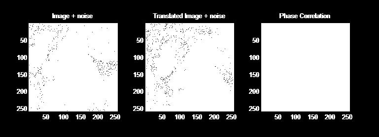
24 Optical Field: Phase Correlation Method [10]

25 Optical Field: Lucas-Kanade Method [8] Assuming that the optical low (V, ) is constant in a small window o size mm with m>1, which is center at (, ) and numbering the piels within as 1 n, n=m 2, a set o equations can be ound: I V I t hogijung@hanang.ac.kr

26 Optical Field: Lucas-Kanade Method [8] c.) Harris corner detector

27 KL Feature racker [11]

28 KL Feature racker [11] F () 로 weighting hogijung@hanang.ac.kr

29 KL Feature racker [11] I V I t KL: An Implementation o the Kanade-Lucas-omasi Feature racker hogijung@hanang.ac.kr

30 Lucas-Kanade Method: A Uniing Framework [12] Since the Lucas-Kanade algorithm was proposed in 1981 image alignment has become one o the most widel used techniques in computer ision. Besides optical low, some o its other applications include - tracking (Black and Jepson, 1998; Hager and Belhumeur, 1998), - parametric and laered motion estimation (Bergen et al., 1992), - mosaic construction (Shum and Szeliski, 2000), - medical image registration (Christensen and Johnson, 2001), - ace coding (Baker and Matthews, 2001; Cootes et al., 1998). hogijung@hanang.ac.kr

31 Lucas-Kanade Method: A Uniing Framework [12] hogijung@hanang.ac.kr

32 Lucas-Kanade Method: A Uniing Framework [12] Minimizing the epression in Equation (1) is a non-linear optimization task een i W(; p) is linear in p because the piel alues I() are, in general, non-linear in. hogijung@hanang.ac.kr

33 Lucas-Kanade Method: A Uniing Framework [12] hogijung@hanang.ac.kr

34 Lucas-Kanade Method: A Uniing Framework [12] hogijung@hanang.ac.kr

35 Lucas-Kanade Method: A Uniing Framework [12] Setting this epression to equal zero and soling gies the closed orm solution or the minimum o the epression in Equation (6) as: SD hogijung@hanang.ac.kr

36 Lucas-Kanade Method: A Uniing Framework [12] hogijung@hanang.ac.kr

37 Lucas-Kanade Method: A Uniing Framework [12] hogijung@hanang.ac.kr

38 Reerences 1. Richard Szeliski, Dense motion estimation, Computer Vision: Algorithms and Applications, 19 June 2009 (drat), pp Emanuele rucco, Alessandro Verri, 8. Motion, Introductor echniques or 3-D Computer Vision, Prentice Hall, New Jerse 1998, pp Wikipedia, Motion ield, aailable on 4. Wikipedia, Optical low, aailable on 5. Alessandro Verri, Emanuele rucco, Finding the Epipole rom Uncalibrated Optical Flow, BMVC 1997, aailable on 6. Wikipedia, Paralle, aailable on 7. Jae Ku Suhr, Ho Gi Jung, Kwanghuk Bae, Jaihie Kim, Outlier rejection or cameras on intelligent ehicles, Pattern Recognition Letters 29 (2008) Wikipedia, Lucas-Kanade Optical Flow Method, aailable on 9. Wikipedia, Aperture Problem, aailable on Wikipedia, Phase correlation, aailable on Wikipedia, Kanade-Lucas-omasi eature tracker, aailable on er 12. Simon Baker, Iain Matthews, Lucas-Kanade 20 ears: A Uniing Framework, International Journal o Computer Vision, 56(3), , hogijung@hanang.ac.kr