Nonlinear Time Series Modeling

Transcription

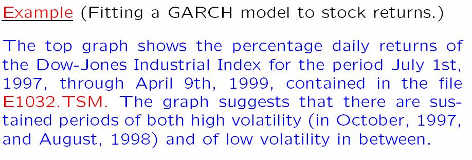
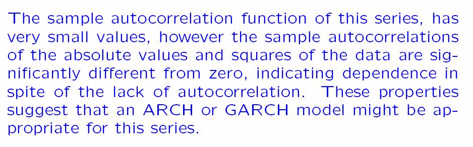
1 Nonlinear Time Series Modeling Part II: Time Series Models in Finance Richard A. Davis Colorado State University ( MaPhySto Workshop Copenhagen September 27 30,

2 Part II: Time Series Models in Finance 1. Classification of white noise 2. Examples 3. Stylized facts concerning financial time series 4. ARCH and GARCH models 5. Forecasting with GARCH 6. IGARCH 7. Stochastic volatility models 8. Regular variation and application to financial TS 8.1 univariate case 8.2 multivariate case 8.3 applications of multivariate regular variation 8.4 application of multivariate RV equivalence 8.5 examples 8.6 Extremes for GARCH and SV models 8.7 Summary of results for ACF of GARCH & SV models 2

3 1. Classification of White Noise As we have already seen from financial data, such as log(returns), and from residuals from some ARMA model fits, one needs to consider time series models for white noise (uncorrelated) that allows for dependence. Classification of WN (in increasing degree of whiteness ). 3

4 1. Classification of White Noise (cont) 4

5 2. Examples (1) All-pass processs. Satisfies W1 and not W2. 5

6 2. Examples (cont) 6

7 2. Examples (cont) 7

8 2. Examples (cont) 8

9 2. Examples (cont) 9

10 2. Examples (cont) 10

11 2. Examples (cont) 11

12 2. Examples (cont) Properties of ARCH(1) process: 1. Strictly stationary solution if 0 < α 1 <1. 2. {Z t } ~ WN(0,α 0 /(1-α 1 )). 3. Not IID since 4. Not Gaussian. 5. Z t has a symmetric distribution (Z 1 = d Z 1 ) 6. EZ t4 < if and only if 3α 12 < 1. (More on moments later.) 7. If EZ t4 <, then the squared process Y t = Z t2 has the same ACF as the AR(1) process W t = α 1 W t-1 + e t 12

13 2. Examples (cont) Likelihood function: 13

14 2. Examples (cont) A realization of the process 14

15 2. Examples (cont) The sample ACF. 15

16 2. Examples (cont) The sample ACF of the absolute values and squares. 16

17 17

18 3. Stylized Facts of Financial Returns Define X t = 100*(ln (P t ) - ln (P t-1 )) (log returns) heavy tailed P( X 1 > x) ~ C x -α, 0 < α < 4. uncorrelated ˆ ρ X ( h) near 0 for all lags h > 0 (MGD sequence?) X t and X t2 have slowly decaying autocorrelations ρˆ ( ) and ˆ X h ρ 2 ( h) process exhibits stochastic volatility. X converge to 0 slowly as h increases. 18

19 Log returns for IBM 1/3/62-11/3/00 (blue= ) 100*log(returns) time 19

20 Sample ACF IBM (a) , (b) (a) ACF of IBM (1st half) (b) ACF of IBM (2nd half) ACF ACF Lag Lag Remark: Both halves look like white noise. 20

21 ACF of squares for IBM (a) , (b) (a) ACF, Squares of IBM (1st half) (b) ACF, Squares of IBM (2nd half) ACF ACF Lag Lag Remark: Series are not independent white noise? 21

22 Plot of M t (4)/S t (4) for IBM M(4)/S(4) Remark: For IID data, M t (k)/s t (k) 0 as t iff E X, k <, where t k k M t = maxs= 1,..., t X s and St = X s t s= 1 22

23 Hill s estimator of tail index The marginal distribution F for heavy-tailed data is often modeled using Pareto-like tails, 1-F(x) = x -α L(x), for x large, where L(x) is a slowly varying function (L(xt)/ L(x) 1, as x ). Now if X~ F, then P(log X > x) = P(X > exp(x))=exp(-αx)l(exp(x)), and hence log X has an approximate exponential distribution for large x. The spacings, log( X (j) ) log(x (j+1) ), j=1,2,...,m, from a sample of size n from an exponential distr are approximately independent and Exp(αj) distributed. This suggests estimating α 1 by αˆ 1 = = 1 m 1 m m ( log X ( j) log X ( j+ 1) ) j= 1 m ( log X ( j) log X ( m+ 1) ) j= 1 j 23

24 Hill s estimator of tail index Def: The Hill estimate of α for heavy-tailed data with distribution given by 1-F(x) = x -α L(x), is αˆ 1 = 1 m m ( log X ( j) log X ( j+ 1) ) j= 1 j = 1 m m ( log X ( j) log X ( m+ 1) ) j= 1 The asymptotic variance of this estimate for α is ˆ 2 2 α / m and estimated by α / m. (See also GPD=generalized Pareto distribution.) 24

25 Hill s plot of tail index for IBM ( , ) Hill Hill m m 25

26 4. ARCH and GARCH Models 26

27 4. ARCH and GARCH Models (cont) 27

28 4. ARCH and GARCH Models (cont) 28

29 4. ARCH and GARCH Models (cont) 29

30 4. ARCH and GARCH Models (cont) 30

31 4. ARCH and GARCH Models (cont) 31

32 4. ARCH and GARCH Models (cont) 32

33 4. ARCH and GARCH Models (cont) 33

34 4. ARCH and GARCH Models (cont) 34

35 4. ARCH and GARCH Models (cont) 35

36 4. ARCH and GARCH Models (cont) 36

37 4. ARCH and GARCH Models (cont) i 37

38 4. ARCH and GARCH Models (cont) 38

39 39

40 4. ARCH and GARCH Models (cont) 40

41 4. ARCH and GARCH Models (cont) SS but not WS GARCH Processes 41

42 4. ARCH and GARCH Models (cont) 42

43 43

44 4. ARCH and GARCH Models (cont) 44

45 4. ARCH and GARCH Models (cont) 45

46 46

47 47

48 48

49 Parameter Estimation for Finite-Variance GARCH Models 49

50 4. ARCH and GARCH Models (cont) 50

51 51

52 52

53 4. ARCH and GARCH Models (cont) 53

54 4. ARCH and GARCH Models (cont) 54

55 4. ARCH and GARCH Models (cont) 55

56 4. ARCH and GARCH Models (cont) 56

57 4. ARCH and GARCH Models (cont) 57

58 4. ARCH and GARCH Models (cont) 58

59 4. ARCH and GARCH Models (cont) 59

60 4. ARCH and GARCH Models (cont) 60

61 4. ARCH and GARCH Models (cont) 61

62 4. ARCH and GARCH Models (cont) 62

63 63

64 4. ARCH and GARCH Models (cont) 64

65 4. ARCH and GARCH Models (cont) 65

66 5. Forecasting with GARCH 66

67 5. Forecasting with GARCH (cont) 67

68 6. IGARCH 68

69 7. Stochastic Volatility Models 69

70 7. Stochastic Volatility Models (cont) 70

71 7. Stochastic Volatility Models (cont) 71

72 7. Stochastic Volatility Models (cont) 72

73 7. Stochastic Volatility Models (cont) 73

74 7. Stochastic Volatility Models (cont) 74

75 7. Stochastic Volatility Models (cont) 75

76 7. Stochastic Volatility Models (cont) 76

77 7. Stochastic Volatility Models (cont) 77

78 7. Stochastic Volatility Models (cont) 78

79 7. Stochastic Volatility Models (cont) 79

80 7. Stochastic Volatility Models (cont) 80

81 81

82 7. Stochastic Volatility Models (cont) 82

83 8. Regular variation and application to financial TS models 8.1 Regular variation univariate case Def: The random variable X is regularly varying with index α if P( X > t x)/p( X >t) x α and P(X> t)/p( X >t) p, or, equivalently, if P(X> t x)/p( X >t) px α and P(X< t x)/p( X >t) qx α, where 0 p 1 and p+q=1. Equivalence: X is RV(α) if and only if P(X t ) /P( X >t) v µ( ) ( v vague convergence of measures on R\{0}). In this case, µ(dx) = (pα x α 1 I(x>0) + qα (-x) -α 1 I(x<0)) dx Note: µ(ta) = t -α µ(a) for every t and A bounded away from 0. 83

84 8.1 Regular variation univariate case (cont) Another formulation (polar coordinates): Define the ± 1 valued rv θ, P(θ = 1) = p, P(θ = 1) = 1 p = q. Then X is RV(α) if and only if or P( X t x, X/ X S) P( X > t ) > α x P( θ S) P( X t x,x/ X ) P( X > t ) > α v x P( θ ) ( v vague convergence of measures on S 0 = {-1,1}). 84

85 8.2 Regular variation multivariate case Multivariate regular variation of X=(X 1,..., X m ): There exists a random vector θ S m-1 such that Equivalence: P( X > t x, X/ X )/P( X >t) v x α P( θ ) ( v vague convergence on S m-1, unit sphere in R m ). P( θ ) is called the spectral measure α is the index of X. P( X t ) v µ ( ) P ( X > t ) µ is a measure on R m which satisfies for x > 0 and A bounded away from 0, µ(xb) = x α µ(xa). 85

86 8.2 Regular variation multivariate case (cont) Examples: 1. If X 1 > 0 and X 2 > 0 are iid RV(α), then X= (X 1, X 2 ) is multivariate regularly varying with index α and spectral distribution P( θ =(0,1) ) = P( θ =(1,0) ) =.5 (mass on axes). Interpretation: Unlikely that X 1 and X 2 are very large at the same time. Figure: plot of (X t1,x t2 ) for realization of 10,000. x_ x_1 86

87 2. If X 1 = X 2 > 0, then X= (X 1, X 2 ) is multivariate regularly varying with index α and spectral distribution P( θ = (1/ 2, 1/ 2) ) = AR(1): X t =.9 X t-1 + Z t, {Z t }~IID symmetric stable (1.8) { ±(1,.9)/sqrt(1.81), W.P Distr of θ: ±(0,1), W.P Figure: plot of (X t, X t+1 ) for realization of 10,000. x_{t+1} x_t 87

88 8.3 Applications of multivariate regular variation Domain of attraction for sums of iid random vectors (Rvaceva, 1962). That is, when does the partial sum 1 a n t= 1 converge for some constants a n? n Spectral measure of multivariate stable vectors. Domain of attraction for componentwise maxima of iid random vectors (Resnick, 1987). Limit behavior of 1 a n n t= 1 Weak convergence of point processes with iid points. Solution to stochastic recurrence equations, Y t = A t Y t-1 + B t Weak convergence of sample autocovariances. X t X t 88

89 8.3 Applications of multivariate regular variation (cont) Linear combinations: X ~RV(α) all linear combinations of X are regularly varying i.e., there exist α and slowly varying fcn L(.), s.t. P(c T X> t)/(t -α L(t)) w(c), exists for all real-valued c, where w(tc) = t α w(c). Use vague convergence with A c ={y: c T y > 1}, i.e., T P( X ta c ) P ( c X > t) = µ (A ) : w( ), c = c α t L ( t) P( X > t ) A c where t -α L(t) = P( X > t). 89

90 8.3 Applications of multivariate regular variation (cont) Converse? X ~RV(α) all linear combinations of X are regularly varying? There exist α and slowly varying fcn L(.), s.t. (LC) P(c T X> t)/(t -α L(t)) w(c), exists for all real-valued c. Theorem (Basrak, Davis, Mikosch, `02). Let X be a random vector. 1. If X satisfies (LC) with α non-integer, then X is RV(α). 2. If X > 0 satisfies (LC) for non-negative c and α is non-integer, then X is RV(α). 3. If X > 0 satisfies (LC) with α an odd integer, then X is RV(α). 90

91 8.4 Applications of theorem 1. Kesten (1973). Under general conditions, (LC) holds with L(t)=1 for stochastic recurrence equations of the form Y t = A t Y t-1 + B t, (A t, B t ) ~ IID, A t d d random matrices, B t random d-vectors. It follows that the distributions of Y t, and in fact all of the finite dim l distrs of Y t are regularly varying (if α is non-even). 2. GARCH processes. Since squares of a GARCH process can be embedded in a SRE, the finite dimensional distributions of a GARCH are regularly varying. 91

92 8.5 Examples Example of ARCH(1): X t =(α 0 +α 1 X 2 t-1) 1/2 Z t, {Z t }~IID. α found by solving E α 1 Z 2 α/2 = 1. α α Distr of θ: P(θ ) = E{ (B,Z) α I(arg((B,Z)) )}/ E (B,Z) α where P(B = 1) = P(B = -1) =.5 92

93 8.4 Examples (cont) Example of ARCH(1): α 0 =1, α 1 =1, α=2, X t =(α 0 +α 1 X 2 t-1) 1/2 Z t, {Z t }~IID Figures: plots of (X t, X t+1 ) and estimated distribution of θ for realization of 10,000. x_{t+1} x_t theta 93

94 8.4 Applications of theorem (cont) Example: SV model X t = σ t Z t Suppose Z t ~ RV(α) and logσ 2 t = j= ψ ε j t j, j= ψ 2 j <,{ ε t }~ IIDN(0, σ 2 ). Then Z n =(Z 1,,Z n ) is regulary varying with index α and so is X n = (X 1,,X n ) = diag(σ 1,, σ n ) Z n with spectral distribution concentrated on (±1,0), (0, ±1). Figure: plot of (X t,x t+1 ) for realization of 10,000. x_ x_1 94

95 8.6 Extremes for GARCH and SV processes Setup X t = σ t Z t, {Z t } ~ IID (0,1) X t is RV (α) Choose {b n } s.t. np(x t > b n ) 1 Then P n ( 1 b X1 x) exp{ x α n }. Then, with M n = max{x 1,..., X n }, (i) GARCH: P( b γ is extremal index ( 0 < γ < 1). (ii) SV model: P( b M x) exp{ γx 1 α n n M x) exp{ x }, 1 α n n }, extremal index γ = 1 no clustering. 95

96 8.6 Extremes for GARCH and SV processes (cont) (i) GARCH: P( b (ii) SV model: P( b M x) exp{ γx 1 α n n M x) exp{ x 1 α n n } } Remarks about extremal index. (i) (ii) γ < 1 implies clustering of exceedances Numerical example. Suppose c is a threshold such that Then, if γ =.5, P( b (iii) 1/γ is the mean cluster size of exceedances. (iv) Use γ to discriminate between GARCH and SV models. (v) P n 1 ( bn X1 1 n M n c) ~.95 c) ~ (.95) =.975 Even for the light-tailed SV model (i.e., {Z t } ~IID N(0,1), the extremal index is 1 (see Breidt and Davis `98 ).5 96

97 8.6 Extremes for GARCH and SV processes (cont) ** * * *** *** time 97

98 8.7 Summary of results for ACF of GARCH(p,q) and SV models GARCH(p,q) α (0,2): α (2,4): α (4, ): d ( ρˆ X ( h)) h=, K, m ( Vh / V0 ) h= 1, K, 1 m 1 2/ α d 1 ( n ρ ( h) ) γ (0)( V ). ˆ X h= 1, K, m X h h= 1, K, m 1/2 d 1 ( n ρ ( h) ) (0)( G ). ˆ X γ h= 1, K, m X h h= 1, K, m, Remark: Similar results hold for the sample ACF based on X t and X t2. 98

99 8.7 Summary of results for ACF of GARCH(p,q) and SV models (cont) SV Model α (0,2): 1/ α d 1 h+ 1 α h ( n / ln n) ρˆ ( h). X σ σ σ 1 2 α S S 0 α (2, ): 1/2 d 1 ( n ρ ( h) ) (0)( G ). ˆ X γ h= 1, K, m X h h= 1, K, m 99

100 Sample ACF for GARCH and SV Models (1000 reps) (a) GARCH(1,1) Model, n= (b) SV Model, n=

101 Sample ACF for Squares of GARCH (1000 reps) (a) GARCH(1,1) Model, n= b) GARCH(1,1) Model, n=

102 Sample ACF for Squares of SV (1000 reps) (c) SV Model, n= (d) SV Model, n=

103 Example: Amazon returns May 16, 1997 to June 16, Series Residual ACF: Abs values Residual ACF: Squares

104 Wrap-up Regular variation is a flexible tool for modeling both dependence and tail heaviness. Useful for establishing point process convergence of heavy-tailed time series. Extremal index γ < 1 for GARCH and γ =1for SV. Unresolved issues related to RV (LC) α = 2n? there is an example for which X 1, X 2 > 0, and (c, X 1 ) and (c, X 2 ) have the same limits for all c > 0. α = 2n 1 and X > 0 (not true in general). 104