BAYESIAN DECISION THEORY. J. Elder CSE 4404/5327 Introduction to Machine Learning and Pattern Recognition

Transcription

1 BAYESIAN DECISION THEORY

2 Credits 2 Some of these slides were sourced and/or modified from: Christopher Bishop, Microsoft UK Simon Prince, University College London Sergios Theodoridis, University of Athens & Konstantinos Koutroumbas, National Observatory of Athens

3 Bayesian Decision Theory: Topics 3 1. Probability 2. The Univariate Normal Distribution 3. Bayesian Classifiers 4. Minimizing Risk 5. The Multivariate Normal Distribution 6. Decision Boundaries in Higher Dimensions 7. Parameter Estimation 8. Mixture Models and EM 9. Nonparametric Density Estimation 10. What are Bayes Nets?

4 Problems for this Meeting 4 Problems Assigned Problem: 2.2

5 Bayesian Decision Theory: Topics 5 1. Probability 2. The Univariate Normal Distribution 3. Bayesian Classifiers 4. Minimizing Risk 5. The Multivariate Normal Distribution 6. Decision Boundaries in Higher Dimensions 7. Parameter Estimation 8. Mixture Models and EM 9. Nonparametric Density Estimation 10. Training and Evaluation Methods 11. What are Bayes Nets?

6 Topic 1. Probability

7 Random Variables 7 A random variable is a variable whose value is uncertain. For example, the height of a randomly selected person in this class is a random variable I won t know its value until the person is selected. Note that we are not completely uncertain about most random variables. For example, we know that height will probably be in the 5-6 range. In addition, 5 6 is more likely than 5 0 or 6 0. The function that describes the probability of each possible value of the random variable is called a probability distribution.

8 Probability Distributions 8 For a discrete distribution, the probabilities over all possible values of the random variable must sum to 1.

9 Probability Distributions 9 For a discrete distribution, we can talk about the probability of a particular score occurring, e.g., p(province = Ontario) = We can also talk about the probability of any one of a subset of scores occurring, e.g., p(province = Ontario or Quebec) = In general, we refer to these occurrences as events.

10 Probability Distributions 10 For a continuous distribution, the probabilities over all possible values of the random variable must integrate to 1 (i.e., the area under the curve must be 1). Note that the height of a continuous distribution can exceed 1! S h a d e d a r e a = S h a d e d a r e a = S h a d e d a r e a =

11 Continuous Distributions 11 For continuous distributions, it does not make sense to talk about the probability of an exact score. e.g., what is the probability that your height is exactly inches? Normal Approximation to probability distribution for height of Canadian females (parameters from General Social Survey, 1991) Probability p µ = s = 5'3.8" 2.6" Height (in)?

12 Continuous Distributions 12 It does make sense to talk about the probability of observing a score that falls within a certain range e.g., what is the probability that you are between 5 3 and 5 7? e.g., what is the probability that you are less than 5 10? Valid events Normal Approximation to probability distribution for height of Canadian females (parameters from General Social Survey, 1991) Probability p µ = s = 5'3.8" 2.6" Height (in)

13 Probability Densities 13 Cumulative distribution (CDF) Probability density (PDF)

14 Transformed Densities 14 Observations falling within ( x +! x ) tranform to the range ( y +!y )! p x (x) "x = p y (y ) "y! p y (y )! p x (x) "x "y Note that in general,!y "!x. Rather,!y!x " dy dx as!x " 0. Thus p y (y ) = p x (x) dx dy

15 Joint Distributions 15 Marginal Probability Joint Probability Conditional Probability

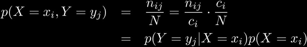
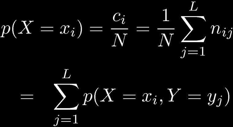
16 Joint Distributions 16 Sum Rule Product Rule

17 Joint Distributions: The Rules of Probability 17 Sum Rule Product Rule

18 Marginalization 18 We can recover probability distribution of any variable in a joint distribution by integrating (or summing) over the other variables

19 Conditional Probability 19 Conditional probability of X given that Y=y* is relative propensity of variable X to take different outcomes given that Y is fixed to be equal to y* Written as Pr(X Y=y*)

20 Conditional Probability 20 Conditional probability can be extracted from joint probability Extract appropriate slice and normalize

21 Conditional Probability 21 More usually written in compact form Can be re-arranged to give

22 Independence 22 If two variables X and Y are independent then variable X tells us nothing about variable Y (and vice-versa)

23 Independence 23 When variables are independent, the joint factorizes into a product of the marginals:

24 Bayes Rule 24 From before: Combining: Re-arranging:

25 Bayes Rule Terminology 25 Likelihood propensity for observing a certain value of X given a certain value of Y Prior what we know about y before seeing x Posterior what we know about y after seeing x Evidence a constant to ensure that the left hand side is a valid distribution

26 End of Lecture 2

27 Bayesian Decision Theory: Topics Probability 2. The Univariate Normal Distribution 3. Bayesian Classifiers 4. Minimizing Risk 5. The Multivariate Normal Distribution 6. Decision Boundaries in Higher Dimensions 7. Parameter Estimation 8. Mixture Models and EM 9. Nonparametric Density Estimation 10. Training and Evaluation Methods 11. What are Bayes Nets?

28 Topic 2. The Univariate Normal Distribution

29 The Gaussian Distribution 29 MATLAB Statistics Toolbox Function: normpdf(x,mu,sigma)

30 Central Limit Theorem 30 The distribution of the sum of N i.i.d. random variables becomes increasingly Gaussian as N grows. Example: N uniform [0,1] random variables.

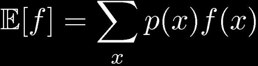
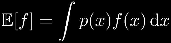
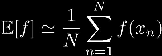
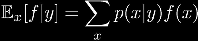
31 Expectations 31 Condi3onal Expecta3on (discrete) Approximate Expecta3on (discrete and con3nuous)

32 Variances and Covariances 32

33 Gaussian Mean and Variance 33

34 Bayesian Decision Theory: Topics Probability 2. The Univariate Normal Distribution 3. Bayesian Classifiers 4. Minimizing Risk 5. The Multivariate Normal Distribution 6. Decision Boundaries in Higher Dimensions 7. Parameter Estimation 8. Mixture Models and EM 9. Nonparametric Density Estimation 10. Training and Evaluation Methods 11. What are Bayes Nets?

35 Topic 3. Bayesian Classifiers

36 Bayesian Classification 36 Input feature vectors x = T!" x 1,x 2,...,x l # $ Assign the pattern represented by feature vector x to the most probable of the available classes! 1,! 2,...,! M That is, x! " i : P(" i x) is maximum. Posterior

37 Bayesian Classification 37 Computation of posterior probabilities Assume known Prior probabilities P(! 1 ),P(! 2 )...,P(! M ) Likelihoods p( x! i ), i = 1,2,,M

38 Bayes Rule for Classification 38 ( ) = p ( x! i )p(! i ) p( x) p! i x where M ( ) = p x! i p x " i=1 ( )p! i ( ),

39 M=2 Classes Given x classify it according to the rule If P(! 1 x) > P(! 2 x) "! 1 If P(! 2 x) > P(! 1 x) "! 2 Equivalently: classify x according to the rule If p( x! 1 )P! 1 If p( x! 2 )P! 2 ( ) > p x! 2 ( ) > p x! 1 ( )P! 2 ( )P! 1 ( ) "! 1 ( ) "! 2 For equiprobable classes the test becomes ( ) > p( x! 2 ) "! 1 ( ) > p( x! 1 ) "! 2 If p x! 1 If p x! 2

40 Example: Equiprobable Classes 40 R ( ω ) and R ( ω )

41 Example: Equiprobable Classes Probability of error The black and red shaded areas represent Thus x 0 ( ) = p(x! 2 )dx P error! 2 $ and P error! 1 "# " ( ) = p(x! 1 )dx # x 0 P e! P(error) = P (! 2 )P error! 2 = 1 2 x 0 $ "# ( ) + P! 1 1 p(x! 2 )dx + 2 +# $ x 0 ( )P error! 1 p(x! 1 )dx ( ) Bayesian classifier is OPTIMAL: it minimizes the classification error probability

42 Example: Equiprobable Classes 42 To see this, observe that shifting the threshold increases the error rate for one class of patterns more than it decreases the error rate for the other class.

43 The General Case In general, for M classes and unequal priors, the decision rule P(! i x) > P(! j x) "j # i $! i minimizes the expected error rate.

44 Types of Error 44 Minimizing the expected error rate is a pretty reasonable goal. However, it is not always the best thing to do. Example: You are designing a pedestrian detection algorithm for an autonomous navigation system. Your algorithm must decide whether there is a pedestrian crossing the street. There are two possible types of error: False positive: there is no pedestrian, but the system thinks there is. Miss: there is a pedestrian, but the system thinks there is not. Should you give equal weight to these 2 types of error?

45 Bayesian Decision Theory: Topics Probability 2. The Univariate Normal Distribution 3. Bayesian Classifiers 4. Minimizing Risk 5. The Multivariate Normal Distribution 6. Decision Boundaries in Higher Dimensions 7. Parameter Estimation 8. Mixture Models and EM 9. Nonparametric Density Estimation 10. Training and Evaluation Methods 11. What are Bayes Nets?

46 Topic 4. Minimizing Risk

47 The Loss Matrix 47 To deal with this problem, instead of minimizing error rate, we minimize something called the risk. First, we define the loss matrix L, which quantifies the cost of making each type of error. Element λ ij of the loss matrix specifies the cost of deciding class j when in fact the input is of class i. Typically, we set λ ii =0 for all i. Thus a typical loss matrix for the M = 2 case would have the form L = " $ $ # 0! 12! 21 0 % ' ' &

48 Risk 48 Given a loss function, we can now define the risk associated with each class k as: M $ i=1 r k =! ki p( x " k )dx # R i Probability we will decide Class! i given pattern from Class! k where R i is the region of the input space where we will decide i.

49 Minimizing Risk 49 Now the goal is to minimize the expected risk r, given by r = M " k=1 r k P (! ) k

50 Minimizing Risk 50 r = M " r k P (! ) k where r k =! ki p( x " k )dx k=1 M $ i=1 # R i We need to select the decision regions R i to minimize the risk r. Note that the set of R i are disjoint and exhaustive. Thus we can minimize the risk by ensuring that each input x falls in the region R i that minimizes the expected loss for that particular input, i.e., M Letting l i = #! ki p ( x " k )P (" ) k, k =1 we select the partioning regions such that x $R i if l i < l j %j & i

51 Example: M=2 51 For the 2-class case: l 1 =! 11 p ( x " 1 )P " 1 and l 2 =! 12 p ( x " 1 )P " 1 Thus we assign x to 1 if i.e., if ( ) +! 21 p x " 2 ( )P " 2 ( ) +! 22 p x " 2 ( ) ( )P " 2 ( ) (! 21 "! ) 22 p ( x # 2 )P (# ) 2 < (! 12 "! ) 11 p ( x # 1 )P (# ) 1 ( ) ( ) > P (! )(" 2 21 # " ) 22 P (! )( 1 " 12 # " ). 11 p x! 1 p x! 2 Likelihood Ratio Test

52 Likelihood Ratio Test 52 ( ) ( ) > P (! )(" 2 21 # " )? 22 P (! )( 1 " 12 # " ). 11 p x! 1 p x! 2 Typically, the loss for a correct decision is 0. Thus the likelihood ratio test becomes ( ) ( ) > P (! )? " 2 ( ) 21. " 12 p x! 1 p x! 2 P! 1 In the case of equal priors and equal loss functions, the test reduces to ( )? ( ) > 1. p x! 1 p x! 2

53 Example 53 Consider a one-dimensional input space, with features generated by normal distributions with identical variance: ( ) ( ) p(x! 1 )! N µ 1," 2 p(x! 2 )! N µ 2," 2 where µ 1 = 0, µ 2 = 1, and! 2 = 1 2 Let s assume equiprobable classes, and higher loss for errors on Class 2, specifically:! 21 = 1,! 12 = 1 2.

54 Results 54 The threshold has shifted to the left why?

55 End of Lecture 3

56 Bayesian Decision Theory: Topics Probability 2. The Univariate Normal Distribution 3. Bayesian Classifiers 4. Minimizing Risk 5. The Multivariate Normal Distribution 6. Decision Boundaries in Higher Dimensions 7. Parameter Estimation 8. Mixture Models and EM 9. Nonparametric Density Estimation 10. Training and Evaluation Methods 11. What are Bayes Nets?

57 Topic 5 The Multivariate Normal Distribution

58 The Multivariate Gaussian 58 MATLAB Statistics Toolbox Function: mvnpdf(x,mu,sigma)

59 Geometry of the Multivariate Gaussian 59 where! " Mahalanobis distance from µ to x Eigenvector equation:!u i = " i u i MATLAB Statistics Toolbox Function: mahal(x,y) where (u i,! i ) are the ith eigenvector and eigenvalue of ". Note that! real and symmetric " # i real. See Appendix B for a review of matrices and eigenvectors.

60 Geometry of the Multivariate Gaussian 60! = Mahalanobis distance from µ to x where (u i,! i ) are the ith eigenvector and eigenvalue of ". or y = U(x - µ)

61 Moments of the Multivariate Gaussian 61 thanks to anti-symmetry of z

62 Moments of the Multivariate Gaussian 62

63 5.1 Application: Face Detection

64 Model # 1: Gaussian, uniform covariance 64 Fit model using maximum likelihood criterion face non-face Pixel 2 Pixel 1 Face Face template 59.1 non-face 69.1

65 Model 1 Results 65 Results based on 200 cropped faces and 200 non-faces from the same database How does this work with a real image? 0.6 Pr(Hit) Pr(False Alarm)

66 Model # 2: Gaussian, diagonal covariance 66 Fit model using maximum likelihood criterion face non-face Pixel 2 Face non-face Pixel 1

67 Model 2 Results 67 Results based on 200 cropped faces and 200 non-faces from the same database Pr(Hit) Diagonal Uniform More sophisticated model unsurprisingly classifies new faces and non-faces better Pr(False Alarm)

68 Model # 3: Gaussian, full covariance 68 Fit model using maximum likelihood criterion PROBLEM: we cannot fit this model. We don t have enough data to estimate the full covariance matrix. N=800 training images D=10800 dimensions Pixel 2 Total number of measured numbers = ND = 800x10,800 = 8,640,000 Pixel 1 Total number of parameters in cov matrix = (D+1)D/2 = (10,800+1)x10,800/2 = 58,325,400

69 Transformed Densities Revisited 69 Observations falling within ( x +! x ) tranform to the range ( y +!y )! p x (x) "x = p y (y ) "y! p y (y )! p x (x) "x "y Note that in general,!y "!x. Rather,!y!x " dy dx as!x " 0. Thus p y (y ) = p x (x) dx dy

70 Problems for this week 70 Problems , , are all good! At least do problem We will talk about this Monday. (Hopefully one of you will present a solution!) Also, MATLAB exercises up to are good. At least do Exercise We will talk about this next week.

71 Bayesian Decision Theory: Topics Probability 2. The Univariate Normal Distribution 3. Bayesian Classifiers 4. Minimizing Risk 5. The Multivariate Normal Distribution 6. Decision Boundaries in Higher Dimensions 7. Parameter Estimation 8. Mixture Models and EM 9. Nonparametric Density Estimation 10. Training and Evaluation Methods 11. What are Bayes Nets?

72 Topic 6. Decision Boundaries in Higher Dimensions

73 ! Decision Surfaces 73 If decision regions R i and R j are contiguous, define! g(x)! P(" i x) # P(" j x) Then the decision surface! separates the two decision regions. g(x) is positive on one side and negative on the other.! R i : P (! i x) > P! j x ( ) + g(x) = 0 g(x) = 0 - R j : P (! j x) > P (! i x) 73

74 Discriminant Functions If f (.) monotonic, the rule remains the same if we use: x! " i if: f (P(" i x )) > f (P(" j x)) # i $ j g i (x)! f (P(" i x)) is a discriminant function In general, discriminant functions can be defined in other ways, independent of Bayes. In theory this will lead to a suboptimal solution However, non-bayesian classifiers can have significant advantages: Often a full Bayesian treatment is intractable or computationally prohibitive. Approximations made in a Bayesian treatment may lead to errors avoided by non-bayesian methods.

75 End of Lecture 4

76 Multivariate Normal Likelihoods Multivariate Gaussian pdf p(x! i ) = (2" ) 1! # i & exp $ 1 2 (x $ µ ) ( i )% # $1 i (x $ µ i ) + ' * µ i = E, - x. / # i = E, - (x $ µ i )(x $ µ i ) % called the covariance matrix. /

77 Logarithmic Discriminant Function p(x! i ) = 1! 1 (2" ) 2 2 # i & exp $ 1 2 (x $ µ ) ( i )% # $1 i (x $ µ i ) + ' * ln(!) is monotonic. Define: ( ( )) = ln p ( x! ) i + ln P(! i ) g i (x) = ln p ( x! i )P! i =! 1 2 (x! µ i )T " i!1 (x! µ i ) + ln P(# i ) + C i where C i =!! 2 ln2$! 1 2 ln " i

78 Quadratic Classifiers 78 g i (x) =! 1 2 (x! µ i )T " i!1 (x! µ i ) + ln P(# i ) + C i Thus the decision surface has a quadratic form. 0.5 For a 2D input space, the decision curves are 0.4 quadrics (ellipses, parabolas, hyperbolas or, in degenerate cases, 0.3 lines)

79 Example: Isotropic Likelihoods g i (x) =! 1 2 (x! µ i )T " i!1 (x! µ i ) + ln P(# i ) + C i Suppose that the two likelihoods are both isotropic, but with different means and variances. Then g i (x) =! 1 2" (x 2 + x ) + 1 i " (µ x + µ x )! 1 2 i 1 1 i2 2 i 2" (µ 2 + µ 2 2 i 1 i2 ) + ln P # i i g i (x)! g j (x) = 0 And will be a quadratic equation in 2 variables. ( ) ( ) + C i

80 Equal Covariances 80 g i (x) =! 1 2 (x! µ i )T " i!1 (x! µ i ) + ln P(# i ) + C i The quadratic term of the decision boundary is given by 1 2 xt! "1 "1 j "! i ( ) x Thus if the covariance matrices of the two likelihoods are identical, the decision boundary is linear.

81 Linear Classifier 81 g i (x) =! 1 2 (x! µ i )T "!1 (x! µ i ) + ln P(# i ) + C i In this case, we can drop the quadratic terms and express the discriminant function in linear form: g i (x) = w i T x + w io w i =! "1 µ i w i 0 = ln P(# i ) " 1 2 µt i!"1 µ i

82 Example 1: Isotropic, Identical Variance 82 g i (x) = w i T x + w io Decision Boundary w i =! "1 µ i w i 0 = ln P(# i ) " 1 2 µt i!"1 µ i! = " 2 I. Then w T (x # x o ) = 0, where w = µ i # µ j, and x o = 1 2 (µ i + µ j ) # " 2 ln P($ i ) P($ j ) µ i # µ j µ i # µ j 2

83 Example 2: Equal Covariance 83 g i (x) = w i T x + w io w i =! "1 µ i w i 0 = ln P(# i ) " 1 2 µt i!"1 µ i g ij (x) = w T (x! x 0 ) = 0 where w =! "1 (µ i " µ j ), x 0 and = 1 2 (µ i x * (x T 1 )!1 2 x) )!1 # + µ j )! ln P(" ) & i % ( $ P(" j )' µ i! µ j µ i! µ j 2 )!1,

84 Minimum Distance Classifiers 84 If the two likelihoods have identical covariance AND the two classes are equiprobable, the discrimination function simplifies: g i (x) =! 1 2 (x! µ i )T " i!1 (x! µ i ) + ln P(# i ) + C i g i (x) =! 1 2 (x! µ i )T "!1 (x! µ i )

85 Isotropic Case 85 In the isotropic case, g i (x) =! 1 2 (x! µ i )T "!1 (x! µ i ) =! 1 2# 2 x! µ i Thus the Bayesian classifier simply assigns the class that minimizes the Euclidean distance d e between the observed feature vector and the class mean. 2 d e = x! µ i

86 !!! General Case: Mahalanobis Distance 86 To deal with anisotropic distributions, we simply classify according to the Mahalanobis distance, defined as! d m = g i (x) = ((x! µ i ) T "!1 (x! µ i )) 1/2 Since the covariance matrix is symmetric, it can be represented as!! = "#" T where! and where! Then we have! the columns v i of! are the eigenvectors of "! is a diagonal matrix whose diagonal elements " i are the corresponding eigenvalues. d 2 m = (x! µ i )T " T #!1 "(x! µ i )

87 General Case: Mahalanobis Distance 87 d 2 m = (x! µ i )T " T #!1 "(x! µ i ) Let x! = " T x. Then the coordinates of x! are the projections of x onto the eigenvectors of #, and we have: ( x! " µ! ) 2 1 i 1 +! + # 1 ( x! "! ) 2 l µ il 2 # l = d m Thus the curves of constant Mahalanobis distance c have ellipsoidal form.

88 Example: 88 Given! 1,! 2 : P(! 1 ) = P(! 2 ) and p(x! 1 ) = N (µ 1, "), p(x! 2 ) = N (µ 2, "), # µ 1 = 0 & # % (, µ $ 0 2 = 3 & # % (, " = & % ( ' $ 3 ' $ ' # classify the vector x = 1.0 & % ( using Bayesian classification: $ 2.2 '! -1 = # % $ 0.95 "0.15 " & ( ' Compute Mahalanobis d m from µ 1, µ 2 : d 2 =! m,1 " 1.0, 2.2 # $! ' " %& # ( = 2.952, d 2 =! m,2 " &2.0, &0.8 $ # $! &2.0 %&1 ' " &0.8 # ( = $ Classify x! " 1. Observe that d E,2 < d E,1

89 Bayesian Decision Theory: Topics Probability 2. The Univariate Normal Distribution 3. Bayesian Classifiers 4. Minimizing Risk 5. The Multivariate Normal Distribution 6. Decision Boundaries in Higher Dimensions 7. Parameter Estimation 8. Mixture Models and EM 9. Nonparametric Density Estimation 10. Training and Evaluation Methods 11. What are Bayes Nets?

90 Topic 7. Parameter Estimation

91 Topic 7.1 Maximum Likelihood Estimation

92 Maximum Likelihood Parameter Estimation Suppose we believe input vectors x are distributed as p(x)! p(x;"), where " is an unknown parameter. Given independent training input vectors X = { x 1, x 2,...x } N we want to compute the maximum likelihood estimate " ML for ". Since the input vectors are independent, we have N p(x ;")! p(x 1, x 2,...x N ;") = # p(x k ;") k =1

93 Maximum Likelihood Parameter Estimation N p(x ;!) = " p(x k ;!) k =1 N Let L(!) " ln p(x ;!) = # ln p(x k ;!) k =1 The general method is to take the derivative of L with respect to!, set it to 0 and solve for! : ˆ! ML : $L(!) $(!) = N $ln p(x k ;!) % = 0 $(!) k =1

94 Properties of the Maximum Likelihood Estimator Let! 0 be the true value of the unknown parameter vector. Then! ML is asymptotically unbiased: lim N"#E[! ML ] =! 0 2! ML is asymptotically consistent: lim E ˆ! ML %! 0 = 0 N"$

95 Example: Univariate Normal 95 Likelihood func3on

96 Example: Univariate Normal 96

97 97 Example: Univariate Normal Thus! ML is biased (although asymptotically unbiased).

98 End of Lecture 5

99 Example: Multivariate Normal 99, the log likeli- Given i.i.d. data hood function is given by

100 Maximum Likelihood for the Gaussian 100 Set the derivative of the log likelihood function to zero, and solve to obtain One can also show that " # $ Recall: If x and a are vectors, then! (!x xt a ) =! (!x a t x) = a % & '

101 Topic 7.1 Bayesian Parameter Estimation

102 Bayesian Inference for the Gaussian (Univariate Case) 102 Assume! 2 is known. Given i.i.d. data, the likelihood function for is given by µ This has a Gaussian shape as a function of µ (but it is not a distribution over ). µ

103 Bayesian Inference for the Gaussian (Univariate Case) 103 Combined with a Gaussian prior over µ, this gives the posterior Completing the square over µ, we see that

104 Bayesian Inference for the Gaussian 104 where Note: Shortcut: p ( µ X ) has the form C exp (!" 2 ). Get " 2 in form aµ 2! 2bµ + c = a(µ! b / a) 2 + const and identify µ N = b / a 1 # N 2 = a

105 Bayesian Inference for the Gaussian 105 Example: µ 0 = 0 µ = 0.8! 2 = 0.1

106 Maximum a Posteriori (MAP) Estimation 106 In MAP estimation, we use the value of µ that maximizes the posterior p µ X µ MAP = µ N. ( ) :

107 Full Bayesian Parameter Estimation 107 In both ML and MAP, we use the training data X to estimate a specific value for the unknown parameter vector, and then use that value for subsequent inference on new observations x: p ( x! ) These methods are suboptimal, because in fact we are always uncertain about the exact value of, and to be optimal we should take into account the possibility that assumes other values.

108 Full Bayesian Parameter Estimation 108 In full Bayesian parameter estimation, we do not estimate a specific value for. Instead, we compute the posterior over, and then integrate it out when computing p x X : ( ) p(x X ) = p(! X ) = " p(x!)p(! X )d! p(x!)p(!) p(x ) N p(x!) = # p(x k!) k =1 = " p(x!)p(!) p(x!)p(!)d!

109 Example: Univariate Normal with Unknown Mean 109 Consider again the case p(x µ)!n ( µ,! ) where! is known and µ! N ( µ 0,! ) 0 We showed that p ( µ X)! N ( 2 µ N,! ) N, where In the MAP approach, we approximate p(x X )! N ( µ N,! 2 ) In the full Bayesian approach, we calculate p(x X ) =! p(x µ)p(µ X ) d µ which can be shown to yield p(x X )! N ( µ N,! 2 2 +! ) N

110 Hints for Exercise Here are some MATLAB functions you may find useful in solving Exercise mnrnd mvnrnd mvnpdf mean cov squeeze sum repmat inv min max zeros ones

111 111 Problem function pe=pr142 %Exercise from PR Matlab Manual m(:,1)=[0 0 0]'; m(:,2)=[1 2 2]'; m(:,3)=[3 3 4]'; S=[ ; ; ]; N=1000; %Part 1 ntrain=mnrnd(n,ones(3,1)/3); %Number of training pts generated by each class ntest=mnrnd(n,ones(3,1)/3); %Number of test pts generated by each class test=[]; mml=zeros(3,3); Smli=zeros(3,3,3); for i=1:3 train=mvnrnd(m(:,i),s,ntrain(i)); %training vectors from class i test=[test;mvnrnd(m(:,i),s,ntest(i))]; %test vectors from class i mml(i,:)=mean(train); %ML estimate of mean for class i Smli(i,:,:)=ntest(i)*cov(train,1);%weighted ML estimate of covariance for class i end Sml=squeeze(mean(Smli)/N); %ML estimate of common covariance %Part 2: Euclidean distance for i=1:3 dsq(:,i)=sum((test-repmat(mml(i,:),n,1)).^2,2); end [m,idx(:,1)]=min(dsq'); %Part 3: Mahalanobis distance for i=1:3 y=test-repmat(mml(i,:),n,1); dsq(:,i)=sum((y*inv(sml)).*y,2); end [m,idx(:,2)]=min(dsq'); %Part 4: Maximum likelihood classifier for i=1:3 p(:,i)=mvnpdf(test,mml(i,:),sml); end [m,idx(:,3)]=max(p'); %Ground truth classes idxgt=[ones(ntest(1),1);2*ones(ntest(2),1);3*ones(ntest(3),1)]; for i=1:3 pe(i)=mean(idx(:,i)~=idxgt); %Error rate for class i end!

112 Bayesian Decision Theory: Topics Probability 2. The Univariate Normal Distribution 3. Bayesian Classifiers 4. Minimizing Risk 5. The Multivariate Normal Distribution 6. Decision Boundaries in Higher Dimensions 7. Parameter Estimation 8. Mixture Models and EM 9. Nonparametric Density Estimation 10. Training and Evaluation Methods 11. What are Bayes Nets?

113 Topic 8 Mixture Models and EM

114 Motivation 114 What do we do if a distribution is not wellapproximated by a standard parametric model?

115 8.1 Intuition

116 Mixtures of Gaussians 116 Combine simple models into a complex model: Component Mixing coefficient K=3

117 Mixtures of Gaussians 117

118 Mixtures of Gaussians 118 Determining parameters log likelihood µ,! and " using maximum Log of a sum; no closed form maximum. Solution: use standard, iterative, numeric optimization methods or the expectation maximization algorithm.

119 End of Lecture 6

120 Hidden Variable Interpretation 120 ( ) = P j N ( 2 x; µ j,! ) j p x P 1, P J, µ 1, µ J,! 1,! J J " = " p(j )p x j j =1 J j =1 ( ) x j = 1 j = 2 j = 3 j x j = 1 j = 2 j = 3 j

121 Hidden Variable Interpretation 121 ( ) = P j N ( 2 x; µ j,! ) j p x P 1, P J, µ 1, µ J,! 1,! J ASSUMPTIONS!! for each training datum x i there is a hidden variable j i.! j i represents which Gaussian x i came from! hence j i takes discrete values! OUR GOAL: To estimate the parameters!: J " = " p(j )p x j j =1 J j =1 ( ) The means µ j The covariances " j The weights (mixing coefficients) P j for all J components of the model. THING TO NOTICE:! x! If we knew the hidden variables j i for the training data it would be easy to estimate parameters just estimate individual Gaussians separately.!! j = 1 j = 2 j = 3 j

122 Hidden Variable Interpretation 122 THING TO NOTICE #2:!! If we knew the parameters! it would very easy to estimate the posterior distribution over each hidden variable j i using Bayes rule:! ( ) = p x j,! p j x,! J " j =1 ( )P j p ( x j,! )P j Pr(j x)! x j = 1 j = 2 j = 3 j j=1! j=2! j=3!

123 Expectation Maximization 123 Chicken and egg problem: could find j 1...N if we knew!! could find! if we knew j 1...N! Solution: Expectation Maximization (EM) algorithm (Dempster, Laird and Rubin 1977) EM for Gaussian mixtures can be viewed as alternation between 2 steps: 1. Expectation Step (E-Step) For fixed! find posterior distribution over responsibilities j 1...N! 2. Maximization Step (M-Step) Now use these posterior probabilities to re-estimate!!

124 8.2 Math

125 Mixture Model 125 Let x k,k = 1, N denote the training input observations, assumed to be independent j k! [1, J ] indicate the component of the mixture from which the observation was drawn (Note that x k is observable but j k is hidden.) Let ( ) represent the unknown parameters we are trying to estimate, where! t = " t, P t " represents the vector of coefficients for the component distributions and P represents the mixing coefficients. Our mixture model is p x k! J ( ) = " P jk p ( x k j k ;!) j =1

126 Q Function 126 We will iteratively estimate!, starting with an initial guess!(0) and monotonically improving our estimate!(t) at successive time steps t. For this purpose, we define a Q function N $ ( ) = E &# P jk log p ( x k j k ;" ) Q!;!(t) % k =1 ' ) ( The Q function represents the expected log likelihood of the training data, given our most recent estimate of the parameters!(t), where the expectation is taken over the possible values of the hidden labels j k.

127 Expectation Step 127 In the E-Step, we calculate the (expected) log probability over the possible parameter values: ( ) = E & P jk log p ( x k j k ;" ) Q!;!(t) $ % N # k =1 N # k =1 ( ) = E $ P jk log p x k j k ;" %& N # k =1 J # j k =1 = P ( j k x k ;!)P jk log p x k j k ;" ' ) ( ' () ( )

128 Maximization Step 128 In the M-Step, we select for our new parameter estimate the value that maximizes this expected log probability:!(t + 1) = arg maxq (!;!(t) )!

129 Example: Mixture of Isotropic Gaussians 129 p ( x k j;! ) = E-Step: 1 ( 2"# 2 j )! 2 % exp ' $ x $ µ k j 2 2# & ' j 2 ( * ) * ( ) = p ( j x k ;!) & " l 2 log# j Q!;!(t) N J ** k =1 j =1 $ % & 2 " 1 2# j 2 x k " µ j 2 ' + log Pj ( )

130 Example: Mixture of Isotropic Gaussians 130 Responsibilities Update Equation: ( ) = p x j;"(t) k J P j x k ;!(t) # j =1 ( )P j (t) p ( x k j;"(t) )P j (t) Parameter Update Equations: 2 0!2 L =5!2 0 (e) 2 µ j (t + 1) = N " k =1 N " k =1 P ( j x k ;!(t) ) x k P ( j x k ;!(t) )! j 2 (t + 1) = N $ k =1 P ( j x k ;"(t) ) x k # µ j (t + 1) 2 l N $ k =1 P ( j x k ;"(t) ) P j (t + 1) = 1 N N " k =1 P ( j x k ;!(t) )

131 Univariate Gaussian Mixture Example 131

132 2-Component Bivariate MATLAB Example CSE 2011Z 2010W 80 Exam grade (%) Assignment grade (%)

133 !! 2-Component Bivariate MATLAB Example 133 %update responsibilities! for i=1:k! end! p(:,i)=alphas(i).*mvnpdf(x,mu(i,:),squeeze(s(i,:,:)));! p=p./repmat((sum(p,2)),1,k);! %update parameters! for i=1:k! end! Nk=sum(p(:,i));! mu(i,:)=p(:,i)'*x/nk;! dev=x-repmat(mu(i,:),n,1);! S(i,:,:)=(repmat(p(:,i),1,D).*dev)'*dev/Nk;! alphas(i)=nk/n;! Exam grade (%) CSE 2011Z 2010W Assignment grade (%)

134 Bivariate Gaussian Mixture Example (a) 1 (b) 1 (c) Samples from p x 0 0 ( k, j k!) Samples from p ( x! k ) Responsibilities P j x ;!(t) k k ( )

135 Expectation Maximization 135 EM is guaranteed to monotonically increase the likelihood. However, since in general the likelihood is nonconvex, we are not guaranteed to find the globally optimal parameters.

136 8.3 Applications

137 Old Faithful Example L = Time to next eruption (min)!2 2 0!2 0 (a) 2 L =2!2 2 0!2 0 (b) 2 L =5!2 2 0!2 0 (c) 2 L = 20!2!2!2!2 0 (d) 2!2 0 (e) 2!2 0 (f) 2 Duration of eruption (min)

138 Face Detection Example: 2 Components 138 Face Model Parameters Non-Face Model Parameters Prior Mean Standard deviation Prior Mean Standard deviation Each component is still assumed to have diagonal covariance. The face model and non-face model have divided the data into two clusters. In each case, these clusters have roughly equal weights. The primary thing that these seem to have captured is the photometric (luminance) variation. Note that the standard deviations have become smaller than for the single Gaussian model as any given data point is likely to be close to one mean or the other.

139 Results for MOG 2 Model Pr(Hit) Pr(False Alarm) MOG 2 Diagonal Uniform Performance improves relative to a single Gaussian model, although it is not dramatic. We have a better description of the data likelihood.

140 MOG 5 Components Prior Mean Face Model Parameters Standard deviation Prior Mean Non-Face Model Parameters Standard deviation

141 MOG 10 Components

142 Results for Mog 10 Model Performance improves slightly more, particularly at low false alarm rates. Pr(Hit) MOG 10 MOG 2 Diagonal Uniform Pr(False Alarm)

143 Background Subtraction 143 Test Image Desired Segmentation GOAL : (i) Learn background model (ii) use this to segment regions where the background has been occluded

144 What if the scene isn t static? 144 Gaussian is no longer a good fit to the data. Not obvious exactly what probability model would fit better.

145 Background Mixture Model 145

146 Background Subtraction Example 146

147 End of Lecture 7

148 Bayesian Decision Theory: Topics Probability 2. The Univariate Normal Distribution 3. Bayesian Classifiers 4. Minimizing Risk 5. The Multivariate Normal Distribution 6. Decision Boundaries in Higher Dimensions 7. Parameter Estimation 8. Mixture Models and EM 9. Nonparametric Density Estimation 10. Training and Evaluation Methods 11. What are Bayes Nets?

149 9. Nonparametric Methods

150 Nonparametric Methods 150 Parametric distribution models are restricted to specific forms, which may not always be suitable; for example, consider modelling a multimodal distribution with a single, unimodal model. You can use a mixture model, but then you have to decide on the number of components, and hope that your parameter estimation algorithm (e.g., EM) converges to a global optimum! Nonparametric approaches make few assumptions about the overall shape of the distribution being modelled, and in some cases may be simpler than using a mixture model.

151 Histogramming 151 Histogram methods partition the data space into distinct bins with widths i and count the number of observations, n i, in each bin. Often, the same width is used for all bins, Δ i = Δ. Δ acts as a smoothing parameter. In a D-dimensional space, using M bins in each dimension will require M D bins! The curse of dimensionality

152 Kernel Density Estimation 152 Assume observations drawn from a density p(x) and consider a small region R containing x such that If the volume V of R is sufficiently small, p(x) is approximately constant over R and The expected number K out of N observations that will lie inside R is given by Thus

153 Kernel Density Estimation 153 Kernel Density Estimation: fix V, estimate K from the data. Let R be a hypercube centred on x and define the kernel function (Parzen window) It follows that and hence

154 Kernel Density Estimation 154 To avoid discontinuities in p(x), use a smooth kernel, e.g. a Gaussian (Any kernel k(u) such that will work.) h acts as a smoother.

155 KDE Example 155

156 Kernel Density Estimation 156 Problem: if V is fixed, there may be too few points in some regions to get an accurate estimate.

157 Nearest Neighbour Density Estimation 157 Nearest Neighbour Density Estimation: fix K, estimate V from the data. Consider a hypersphere centred on x and let it grow to a volume V* that includes K of the given N data points. Then for j=1:np! d=sort(abs(x(j)-xi));! V=2*d(K(i));! phat(j)=k(i)/(n*v);! end!

158 Nearest Neighbour Density Estimation 158 Nearest Neighbour Density Estimation: fix K, estimate V from the data. Consider a hypersphere centred on x and let it grow to a volume V* that includes K of the given N data points. Then K=5 K=10 K=100 True distribution Training data KNN Estimate

159 Nearest Neighbour Density Estimation 159 Problem: does not generate a proper density (for example, integral is unbounded on! D ) In practice, on finite domains, can normalize. But makes strong assumption on tails "! 1 % # $ x& '

160 Nonparametric Methods 160 Nonparametric models (not histograms) require storing and computing with the entire data set. Parametric models, once fitted, are much more efficient in terms of storage and computation.

161 K-Nearest-Neighbours for Classification 161 Given a data set with N k data points from class C k and, we have and correspondingly Since, Bayes theorem gives

162 K-Nearest-Neighbours for Classification 162 K = 3 K = 1

163 K-Nearest-Neighbours for Classification 163 K acts as a smother As, the error rate of the 1-nearestneighbour classifier is never more than twice the optimal error (obtained from the true conditional class distributions).

164 KNN Example 164

165 Naïve Bayes Classifiers 165 All of these nonparametric methods require lots of data to work. If O ( N ) training points are required for accurate estimation in 1 dimension, then O ( N D ) points are required for D-dimensional input vectors. It may sometimes be possible to assume that the individual dimensions of the feature vector are conditionally independent. Then we have ( ) = p x j! i p x! i D " j =1 ( ) This reduces the data requirements to O ( DN ).

166 End of Lecture 8

167 Bayesian Decision Theory: Topics Probability 2. The Univariate Normal Distribution 3. Bayesian Classifiers 4. Minimizing Risk 5. The Multivariate Normal Distribution 6. Decision Boundaries in Higher Dimensions 7. Parameter Estimation 8. Mixture Models and EM 9. Nonparametric Density Estimation 10. Training and Evaluation Methods 11. What are Bayes Nets?

168 10. Training and Evaluation Methods

169 Machine Learning System Design 169 The process of solving a particular classification or regression problem typically involves the following sequence of steps: 1. Design and code promising candidate systems 2. Train each of the candidate systems (i.e., learn the parameters) 3. Evaluate each of the candidate systems 4. Select and deploy the best of these candidate systems

170 Using Your Training Data 170 You will always have a finite amount of data on which to train and evaluate your systems. The performance of a classification system is often data-limited: if we only had more data, we could make the system better. Thus it is important to use your finite data set wisely.

171 Overfitting 171 Given that learning is often data-limited, it is tempting to use all of your data to estimate the parameters of your models, and then select the model with the lowest error on your training data. Unfortunately, this leads to a notorious problem called over-fitting.

172 Example: Polynomial Curve Fitting 172

173 Sum-of-Squares Error Function 173

174 How do we choose M, the order of the model? 174

175 1 st Order Polynomial 175

176 3 rd Order Polynomial 176

177 9 th Order Polynomial 177

178 Over-fitting 178 Root Mean Square (RMS) Error:

179 Overfitting and Sample Size th Order Polynomial

180 Over-fitting and Sample Size th Order Polynomial

181 Methods for Preventing Over-Fitting 181 Bayesian parameter estimation Application of prior knowledge regarding the probable values of unknown parameters can often limit over-fitting of a model Model selection criteria Methods exist for comparing models of differing complexity (i.e., with different types and numbers of parameters) Bayesian Information Criterion (BIC) Akaike Information Criterion (AIC) Cross-validation This is a very simple method that is universally applicable.

182 Cross-Validation 182 The available data are partitioned into disjoint training and test subsets. Parameters are learned on the training sets. Performance of the model is then evaluated on the test set. Since the test set is independent of the training set, the evaluation is fair: models that overlearn the noise in the training set will perform poorly on the test set.

183 Cross-Validation: Choosing the Partition 183 What is the best way to partition the data? A larger training set will lead to more accurate parameter estimation. However a small test set will lead to a noisy performance score. If you can afford the computation time, repeat the training/test cycle on complementary partitions and then average the results. This gives you the best of all worlds: accurate parameter estimation and accurate evaluation. In the limit: the leave-one-out method

184 Bayesian Decision Theory: Topics Probability 2. The Univariate Normal Distribution 3. Bayesian Classifiers 4. Minimizing Risk 5. The Multivariate Normal Distribution 6. Decision Boundaries in Higher Dimensions 7. Parameter Estimation 8. Mixture Models and EM 9. Nonparametric Density Estimation 10. Training and Evaluation Methods 11. What are Bayes Nets?

185 10. What are Bayes Nets?

186 Directed Graphical Models and the Role of Causality 186 Bayes nets are directed acyclic graphs in which each node represents a random variable. Arcs signify the existence of direct causal influences between linked variables. Strengths of influences are quantified by conditional probabilities where pa k is the set of 'parent' nodes of node k. NB: For this to hold it is critical that the graph be acyclic.

187 Bayesian Networks 187 Directed Acyclic Graph (DAG) From the definition of conditional probabilities (product rule): In general: This corresponds to a complete graph.

188 Bayesian Networks 188 However, many systems have sparser causal relationships between their variables. General Factorization

189 Generative Models of Perception 189

190 Discrete Variables 190 General joint distribution: K 2-1 parameters Independent joint distribution: 2(K -1) parameters

191 Discrete Variables 191 General distributions require many parameters. General joint distribution over M variables: K M -1 parameters It is thus extremely important to identify structure in the system that corresponds to a sparser graphical model and hence fewer parameters.

192 Binary Variable Example S: Smoker? C: Cancer? H: Heart Disease? (H1, H2): Results of medical tests for heart disease (C1, C2): Results of medical tests for cancer

193 Discrete Variables 193 Example: M -node Markov chain K -1 + (M -1) K(K -1) parameters

194 Using Bayes Nets Once a DAG has been constructed, the joint probability can be obtained by multiplying the marginal (root nodes) and the conditional (non-root nodes) probabilities. Training: Once a topology is given, probabilities are estimated via the training data set. There are also methods that learn the topology. Probability Inference: This is the most common task that Bayesian networks help us to solve efficiently. Given the values of some of the variables in the graph, known as evidence, the goal is to compute the conditional probabilities for some of the other variables, given the evidence.

195 Inference in Bayes Nets 195 In inference, we clamp some of the variables to observed values, and then compute the posterior over other, unobserved variables. Simple example:

196 Example 196 a) Suppose x has been measured and its value is 1. What is the probability that w is 0? b) Suppose w is measured and its value is 1. What is the probability that x is 0?

197 Message Passing For a), computation propagates from node x to node w, resulting in P(w0 x1) = For b), computation propagates in the opposite direction, resulting in P(x0 w1) = 0.4. In general, the required inference information is computed via a combined process of message passing among the nodes of the DAG. Complexity: For singly connected graphs, message passing algorithms amount to a complexity linear in the number of nodes.

198 Bayesian Decision Theory: Topics Probability 2. The Univariate Normal Distribution 3. Bayesian Classifiers 4. Minimizing Risk 5. The Multivariate Normal Distribution 6. Decision Boundaries in Higher Dimensions 7. Parameter Estimation 8. Mixture Models and EM 9. Nonparametric Density Estimation 10. What are Bayes Nets?