Walkthrough for Illustrations. Illustration 1

Transcription

1 Tay, L., Meade, A. W., & Cao, M. (in press). An overview and practical guide to IRT measurement equivalence analysis. Organizational Research Methods. doi: / Walkthrough for Illustrations Illustration 1 File Name Simulated_DData.csv Comment Contains simulated data of 2000 individuals. Group = 1 represents the reference group (N = 1000); Group = 2 represents the focal group (N =1000); I1 to I15 represents items 1 to 15. See the simulated item parameters below (Table 8 in paper). Simulated_DData.irtpro Simulated_DData.SSIG Simulated_DData.Model0-irt Simulated_DData.Model1-irt Simulated_DData.Model2-irt Simulated_DData.Model3-irt Simulated_DData.Model4-irt IRTPRO syntax file IRTPRO data file (converted from the.csv file) Model 0 Output Simultaneous estimation (no constraints) Model 1 Output Fully constrained model Model 2 Output Testing anchor items with two-step procedure Model 3 Output Testing non-anchor items for DIF Model 4 Output Further testing non-anchor items for DIF Table 8. Illustration 1: Simulated item and theta parameters Group = 1 (θ mean =0, θ SD = 1) Group = 2 (θ mean =0.2, θ SD = 1) λ γ a b λ γ a b Type of DIF Large ab DIF Large ab DIF Large ab DIF Large ab DIF

2 STEP 1: Creating SSIG file (IRTPRO data file) A. Click on Start New Project B. Select the data file. In this case, we have Simulated_DData.csv as our raw data. Then click OK

3 C. We have 17 variables here: ID, Group, and 15 item responses. Also we have our Variable names at the top of the file. Click OK D. Check that the data is correctly read in.

4 STEP 2: Analyze data using simultaneous estimation (i.e., simultaneous calibration) of both groups (Model 0) A. Because we are conducting a unidimensional IRT analysis, we select: Analysis > Unidimensional IRT B. Optional: You can fill in the Title for the analysis and Comments to keep track of what model you specify. *Note: You do not need to select the data file as that is already selected even though it appears blank

5 C. In the Group tab, add the Group variable to the Group: box. The tells IRTPRO that there are multiple groups ( >=2) in the data. *Note: The first group is automatically selected as the reference group as shown in the check box.

6 D. In the Items tab, we select all the item variables into the Items: box. This tells IRTPRO which items we want to analyze Then we click on Apply to all groups. This tells IRTPRO that the same set of items were administered across both groups (Group 1 and Group 2). After clicking Apply to all groups, a box will appear Previous settings will be lost. Do you want to continue?. Click Yes

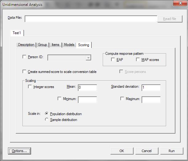
7 E. In the Models tab, we can specify which items to test for DIF and which items (and item parameters) to constrain as equal across groups. For the first analysis, we do not need to specify and DIF analysis or constraints. We note that because the data are dichotomous the model is 2PL by default. F. In the Scoring tab, we do not need to do anything as we are not interested in scoring participants. However, if one is interested to do so, one should specify the Person ID, select the type of scoring method: EAP or MAP scores. The results of EAP or MAP are quite similar and EAP is used more often.

8 G. Finally, to obtain the overall fit statistics (i.e., M 2 and RMSEA), we will need to go into Options In the Options menu, select the Miscellaneous tab. Check the Compute limited-information overall model fit statistics. Note. when checking this box, a text box will appear warning that this can take a long time: This can take a long time if the number of items and/or dimensions is large. Click OK. Then Apply and OK H. After specifying all the necessary model information we can Run the analysis.

9

10 STEP 3: Interpreting output (for Model 0) The output will be produced in a html format Overview: Content -2PL model item parameter estimates for Group 1-2PL model item parameter estimates for Group 2 -Summed-Score Based Item Diagnostic Tables and χ 2 s for Group 1 -Summed-Score Based Item Diagnostic Tables and χ 2 s for Group 2 -Marginal fit (χ 2 ) and standardized LD χ 2 statistics for Group 1 -Marginal fit (χ 2 ) and standardized LD χ 2 statistics for Group 2 -Likelihood-based values and goodness of fit statistics -Factor loadings for Group 1 -Factor loadings for Group 2 -Group parameter estimates -Item information function values for Group 1 -Item information function values for Group 2 -Summary of the data and control parameters Comment 2PL item parameter estimates for Groups 1 and 2 This shows the S- χ 2 where we can examine individual item fit This shows the standardized LD χ 2 statistics we can examine violations of unidimensionality for pairs of items This shows the M 2 and RMSEA value. We can also obtain different information criteria. We specified Factor Loadings in the Options tab in Step 2G. This produces factor loadings. This shows the estimated focal group latent trait distribution (mean & SD). The reference group is usually constrained as N(0,1). This is the discretized information function for items This displays what data were analyzed and estimation information

11 Some things to note when interpreting the output A. The IRTPRO item parameter estimates are: [ ( )] Because we simulated item parameters in with a scaling factor of [ ( )] The IRTPRO item parameter estimates for the a-parameter ( ) is our simulated item parameter multiplied by Here, we see that multiplying the simulated a-parameter by leads produces values similar to the IRTPRO estimates. We also need to check that the s.e s for the items are small showing that the estimates are fairly accurate. a b a*

12 B. The S- χ 2 statistic shows the fit of each individual item. We hope to see that the modeled and the observed frequencies are not significantly different, implying that there is good/reasonable model-data fit. There may be several items that show misfit but a majority of the items should fit well for the specified IRT model. Otherwise, a different model should be considered. C. Group parameter estimates show the estimated latent trait mean and variance (and sd) for the reference group. In this case G1 is the reference group which has the mean and sd fixed at 0 and 1, respectively.

13 D. The standardized LD χ 2 statistics we can examine violations of unidimensionality for pairs of items. Generally, absolute values smaller than 3 indicate good fit. IRTPRO differentiates the magnitude of the standardized LD χ 2 using different shades of colors. Red represents negative associations beyond the single latent trait; blue represents positive associations beyond the single latent trait. Brighter colors indicate larger magnitudes. E. The likelihood-based values and GOF statistics show the AIC, BIC, M 2, and RMSEA for the fitted model

14 STEP 4: Analyze data using simultaneous estimation (i.e., simultaneous calibration) of both groups: Constraining item parameters to be equal across groups (Model 1) Follow the same procedure in STEP 2 (A) through (H). For part (E), click on Constraints Click on Set parameters equal across groups > OK Then RUN This produces a model in which all items are constrained to be equal across groups.

15 STEP 5: Analyze data using simultaneous estimation (i.e., simultaneous calibration) of both groups: Testing all items for DIF using two-step procedure (Model 2) Follow the same procedure in STEP 2 (A) through (H). For part (E), click on DIF Select Test all items, anchor all items > OK Then OK > RUN This produces a model in all items are tested for DIF using a two-step procedure. In the first step, all items are assumed to be invariant to estimate focal group latent trait mean and SD. Then, in the next step, all items are freely estimated and focal group latent trait mean and SD are set at the previously estimated values.

16 In this model, we see that the latent traits are not estimated but fixed. No standard errors are produced for the focal group (Group 2). Further, we examine the p-values for the Wald χ 2 statistic that tests the difference between reference and focal group item parameters (a* & b). We select items that do not have significant DIF as anchor items for our next model (alpha =.05). This includes items 1, 4, 5, 6, 9, 10, 13, &14.

17 STEP 6: Analyze data using simultaneous estimation (i.e., simultaneous calibration) of both groups: Using anchor items found in Model 2 (Model 3) Follow the same procedure in STEP 2 (A) through (H). For part (E), click on DIF Select Test candidate items, estimate group difference with anchor items Drag all anchor items to the Anchor items: box. And all items into Candidate items: box.

18 Then OK > RUN This tests for a model in which non-anchor items are tested for DIF. As shown below, we find the focal group trait mean and SD estimated using the anchor items. Further, the DIF statistics show that there are a number of non-anchor items that do not have significant DIF (alpha =.05). These include items 2, 8, & 12. We add these as our anchor items at the next step.

19 STEP 7: Analyze data using simultaneous estimation (i.e., simultaneous calibration) of both groups: Using anchor items found in Model 3 (Model 4) Follow the same procedure in STEP 6 (A) through (H). Select the anchor items: 1,2,4,5,6,8,9,10,12,13,14. Test all the other items for DIF. As shown in the output below, we find that all the non-anchor items have significant DIF. The iterative procedure ends at this point.

20 Illustration 2 File Name Simulated_PData.csv Comment Contains simulated data of 2000 individuals. Group = 1 represents the reference group (N = 1000); Group = 2 represents the focal group (N =1000); I1 to I15 represents items 1 to 15. See the simulated item parameters below (Table 8 in paper). Simulated_PData.irtpro Simulated_PData.SSIG Simulated_PData.Model0-irt Simulated_PData.Model1-irt Simulated_PData.Model2-irt Simulated_PData.Model3-irt Simulated_PData.Model4-irt Simulated_PData.Model5-irt IRTPRO syntax file IRTPRO data file (converted from the.csv file) Model 0 Output Simultaneous estimation (no constraints) Model 1 Output Fully constrained model Model 2 Output Testing anchor items with two-step procedure Model 3 Output Testing non-anchor items for DIF Model 4 Output Further testing non-anchor items for DIF Model 5 Output Further testing non-anchor items for DIF using different contrasts Table 10. Illustration 2: Simulated item and theta parameters Group 1 (θ mean = 0; θ sd = 1) Group 2 (θ mean = 0; θ sd = 1) Group 3 (θ mean = -.30; θ sd = 1) a b1 b2 b3 b4 a b1 b2 b3 b4 Type of DIF a b1 b2 b3 b Large ab DIF Large ab DIF Small ab DIF Small a DIF Small b DIF Small ab DIF Type of DIF Large ab DIF Large a DIF Large b DIF Small ab DIF Small a DIF Small b DIF Small ab DIF

21 The same steps shown for Illustration 1 are used. The three main differences are: (i) In STEP 2 (E), for the Models tab, the graded response model (GRM) is selected (by default) instead of the 2PLM as the responses are polytomous (ii) The testing of DIF in subsequent steps requires the use of contrasts as there are multiple groups. The default two contrasts are Contrast Group 1 (Reference Group) Group 2 (Focal Group 1) Group 3 (Focal Group 2) Comment Tests whether item parameters in Group 1 differ from Group 2 and Tests whether item parameters in Group 2 differ from Group 3

22 The DIF output shows the Wald χ 2 statistic and the associated p-value for the two contrasts. When selecting anchor items, we want to select items that do not show significant p-values for both contrasts. In this sample of 8 items, we see that items 1, 2, and 8 have non-significant p-values across both contrasts. (iii) Another difference is that we also specify DIF contrasts apart from using the default values. In the Models Tab > DIF > Group contrasts In our illustration, we used the default two contrasts and then used contrasts 3 and 4 to test whether item parameters differ between reference and specific focal groups. Contrast Group 1 (Reference Group) Group 2 (Focal Group 1) Group 3 (Focal Group 2) Comment Tests whether item parameters in Group 1 differ from Group Tests whether item parameters in Group 1 differ from Group 3

23 Illustration 3 File Name Data.sav Data_Restructure.sav Data_Restructure.LGS Simulated_3PL-irt.htm Comment Contains simulated data of 5000 individuals. X1 is a dichotomous grouping variable (0, 1) (e.g., gender, Black-White, etc.); X2 is a continuous variable (e.g., age, income, etc.). Restructured Data.sav for 3PLM IRT analysis in LG Latent GOLD syntax IRTPRO output Running IRTPRO to examine model-data fit The steps for running IRTPRO to examine model data fit are in line with Illustrations 1 and 2. The difference is that in Illustration 3 we are specifying a 3PLM. As such, in the Models tab, we need to change the 2PL to 3PL. This can be done by highlighting all the items and right clicking for additional models. Then we choose 3PL. For a 3PLM, it is helpful to specify priors for the c-parameter otherwise it is usually poorly estimated (large standard errors). We can specify a Beta distribution (α, β) for a c-prior. It has been recommended that the values chosen for the Beta distribution are based on these equations: α=mp+1 and β=m(1-p)+1 (Harwell & Baker, 1991). The value of m would range from 15 to 20 depending on the confidence one has in the prior information (higher values indicate higher levels of confidence). In BILOG, m is set at 20 by default. This is the value we use as well. The value of

24 p is 1/Noptions, where Noptions denotes the number of response options there are. For example, if there are 5 options on the test, p = 1/5 =.20. There is on average a 20% chance of getting an answer correct with random guessing. Therefore, α = mp + 1 =5; β = m(1-p) + 1=17. To set the priors, go to Options Then click on the Priors tab > Enter prior parameters Highlight the entire third column of g values. This represents the c-parameters for the 3PLM. Then right click to choose the Beta distribution

25 Enter the desired values for the Beta distribution

26 Running Latent GOLD for DIF analysis STEP 1: Understanding the LG parameterization The parameterization for Latent GOLD is different from the parameterization used to simulate the item parameters. In addition, the simulated latent trait values need to be rescaled. We simulated item parameters in with a scaling factor of ( ) In addition, the value simulated is not standardized. ( ) ( ) + e Because in the estimation, the latent trait distribution is fixed at N(0,1), we need to divide SD of, which in this case, the expected value is.58. by the ( ) ( ) + e ( ) ( ) + e In the response equation, ( ) ( ) ( ) ( ) where = =

27 Item parameter conversions from Simulated Item parameters to LG item parameters Simulated Item parameters Reparameterized into LG parameters a b c d e a* b* c* d* e* STEP 2: Preparing the data for LG analysis Because the 3PLM is unique in that it has a guessing parameter, we need to structure the data in a unique format so that we can use generalized latent variable modeling. Specifically, we need to have a long and wide format for this analysis. Specifically, if we have 4 items Y1 to Y4, ID Y1 Y2 Y3 Y We will need to restructure it to the following ID itemnr response Y1 Y2 Y3 Y

28 The SPSS syntax is as follows: VARSTOCASES /ID=case /MAKE response FROM y1 y2 y3 y4 y5 y6 y7 y8 y9 y10 y11 y12 y13 y14 y15 /INDEX=itemnr(15) /KEEP=x1 x2 ID /NULL=KEEP. IF itemnr = 1 y1 = response. IF itemnr = 2 y2 = response. IF itemnr = 3 y3 = response. IF itemnr = 4 y4 = response. IF itemnr = 5 y5 = response. IF itemnr = 6 y6 = response. IF itemnr = 7 y7 = response. IF itemnr = 8 y8 = response. IF itemnr = 9 y9 = response. IF itemnr = 10 y10 = response. IF itemnr = 11 y11 = response. IF itemnr = 12 y12 = response. IF itemnr = 13 y13 = response. IF itemnr = 14 y14 = response. IF itemnr = 15 y15 = response. EXECUTE. Using this restructured data, we can then proceed to analyze it in Latent GOLD. For other models without the guessing parameter such as the 1PLM, 2PLM, and GRM, we do not need to have this unique format. We will show some example syntax for these other models in the last section.

29 STEP 3: LG 3PL DIF analysis The proposed procedure is based on research of the IRT-C DIF analysis (Tay, Newman, & Vermunt, 2011; Tay, Vermunt, & Wang, 2013). To open the data file in Latent GOLD, we click on Open symbol and select the restructured data file. In this case, we have labeled our restructured data Data_Restructure.sav. After selecting the file, we should see that it is read in. Then right click on Model1

30 We should see a drop down box after right clicking Model1. Select Generate Syntax as we want to use the Syntax mode. We should now see that there is syntax in the black space that we can edit.

31 For a fully constrained model where all items are constrained as equal across groups options algorithm bhhh tolerance=1e-008 emtolerance=0.01 emiterations=1000 nriterations=500; startvalues seed=0 sets=0 tolerance=1e-005 iterations=50; bayes categorical=1 variances=1 latent=1 poisson=1; montecarlo seed=0 replicates=500 tolerance=1e-008; quadrature nodes=30; missing includeall; output parameters=first standarderrors=fast estimatedvalues bivariateresiduals; variables caseid id; dependent y1, y2, y3, y4, y5, y6, y7, y8, y9, y10, y11, y12, y13, y14, y15; independent itemnr nominal, x1, x2 rank=5; latent theta continuous, c dynamic nominal 2; equations (1) theta; theta <- x1 + x2 ; c <- 1 itemnr; y1 <- 1 + (+) theta + (100) c; y2 <- 1 + (+) theta + (100) c; y3 <- 1 + (+) theta + (100) c; y4 <- 1 + (+) theta + (100) c; y5 <- 1 + (+) theta + (100) c; y6 <- 1 + (+) theta + (100) c; y7 <- 1 + (+) theta + (100) c; y8 <- 1 + (+) theta + (100) c; y9 <- 1 + (+) theta + (100) c; y10 <- 1 + (+) theta + (100) c; y11 <- 1 + (+) theta + (100) c; y12 <- 1 + (+) theta + (100) c; y13 <- 1 + (+) theta + (100) c; y14 <- 1 + (+) theta + (100) c; y15 <- 1 + (+) theta + (100) c;

32 In the parameter tab, the estimated regression weights for the group characteristics (x1 and x2) and the item parameters a* values and b* values are displayed Here, we see that being in X1 (0 = reference; 1 = focal) is associated with -.26 lower latent trait. Here, we see that have a higher value in X2 (which is standardized) for 1SD is associated with.49 higher latent trait. For the first item, the b* value is.85; the a* value is 1.94 b* for item 1 a* for item 1

33 In addition, the estimated c values are diplayed in the Estimated-Values Model. In this case, Item1 c-parameter is estimated at To test for DIF, we examine the output to look for the highest BVR for the item-covariate pair. In this case, it is Item13 and X2, with a BVR value of

34 We then proceed to create a model where we allow for DIF for Item13 on covariate X2. This is done by right clicking Model 1 followed by Copy Model which automatically generates Model 2 with the same exact syntax as Model 1 for editing. We edit the equations for Model 2 by adding X2 to equation y13. This effective models for uniform DIF of item 13 on X2. This revised equation shows that responses on y13 are not merely a function of the underlying theta trait value, but also dependent on group characteristic X2 (e.g., income, GPA, socioeconomic status, etc.). equations (1) theta; theta <- x1 + x2 ; c <- 1 itemnr; y1 <- 1 + (+) theta + (100) c; y2 <- 1 + (+) theta + (100) c; y3 <- 1 + (+) theta + (100) c; y4 <- 1 + (+) theta + (100) c; y5 <- 1 + (+) theta + (100) c; y6 <- 1 + (+) theta + (100) c; y7 <- 1 + (+) theta + (100) c; y8 <- 1 + (+) theta + (100) c; y9 <- 1 + (+) theta + (100) c; y10 <- 1 + (+) theta + (100) c; y11 <- 1 + (+) theta + (100) c; y12 <- 1 + (+) theta + (100) c; y13 <- 1 + (+) theta + x2 + (100) c; y14 <- 1 + (+) theta + (100) c; y15 <- 1 + (+) theta + (100) c; We run this model to examine whether the parameter associated with X2 on the equation y13 <- 1 + (+) theta + x2 + (100) c; is significant, demonstrating the uniform DIF is significant.

35 In the Parameters tab, we can scroll down to see that is the DIF parameter for X2 and it is significantly different from zero at 3.7e-16. Because it is significant, we then proceed to examine the BVRs again to look for the next itemcovariate pair that has the largest BVR. We continue testing for DIF in this manner until we find that the highest flagged BVR value is no longer significant.

36 Syntax for 1PLM (No DIF) equations (1) theta; theta <- x1 + x2 ; y1 <- 1 + (1) theta; y2 <- 1 + (1) theta; y3 <- 1 + (1) theta; y4 <- 1 + (1) theta; y5 <- 1 + (1) theta; y6 <- 1 + (1) theta; y7 <- 1 + (1) theta; y8 <- 1 + (1) theta; y9 <- 1 + (1) theta; y10 <- 1 + (1) theta; y11 <- 1 + (1) theta; y12 <- 1 + (1) theta; y13 <- 1 + (1) theta; y14 <- 1 + (1) theta; y15 <- 1 + (1) theta; Syntax for 1PLM (DIF on Item 13 for covariate x1) equations (1) theta; theta <- x1 + x2 ; y1 <- 1 + (1) theta; y2 <- 1 + (1) theta; y3 <- 1 + (1) theta; y4 <- 1 + (1) theta; y5 <- 1 + (1) theta; y6 <- 1 + (1) theta; y7 <- 1 + (1) theta; y8 <- 1 + (1) theta; y9 <- 1 + (1) theta; y10 <- 1 + (1) theta; y11 <- 1 + (1) theta; y12 <- 1 + (1) theta; y13 <- 1 + (1) theta + x1; y14 <- 1 + (1) theta; y15 <- 1 + (1) theta;

37 Syntax for 2PLM (No DIF) equations (1) theta; theta <- x1 + x2 ; y1 <- 1 + (+) theta; y2 <- 1 + (+) theta; y3 <- 1 + (+) theta; y4 <- 1 + (+) theta; y5 <- 1 + (+) theta; y6 <- 1 + (+) theta; y7 <- 1 + (+) theta; y8 <- 1 + (+) theta; y9 <- 1 + (+) theta; y10 <- 1 + (+) theta; y11 <- 1 + (+) theta; y12 <- 1 + (+) theta; y13 <- 1 + (+) theta; y14 <- 1 + (+) theta; y15 <- 1 + (+) theta; Syntax for 2PLM (DIF on Item 13 for covariate x1) equations (1) theta; theta <- x1 + x2 ; y1 <- 1 + (+) theta; y2 <- 1 + (+) theta; y3 <- 1 + (+) theta; y4 <- 1 + (+) theta; y5 <- 1 + (+) theta; y6 <- 1 + (+) theta; y7 <- 1 + (+) theta; y8 <- 1 + (+) theta; y9 <- 1 + (+) theta; y10 <- 1 + (+) theta; y11 <- 1 + (+) theta; y12 <- 1 + (+) theta; y13 <- 1 + (+) theta + x1; y14 <- 1 + (+) theta; y15 <- 1 + (+) theta;

38 Note: the Graded response model equations are the same for the 2PLM. The only difference is that the responses are cumlogit. variables dependent y1 cumlogit, y2 cumlogit, y3 cumlogit, y4 cumlogit, y5 cumlogit, y6 cumlogit, y7 cumlogit, y8 cumlogit, y9 cumlogit, y10 cumlogit, y11 cumlogit, y12 cumlogit, y13 cumlogit, y14 cumlogit, y15 cumlogit; independent itemnr nominal, x1, x2 rank=5; latent theta continuous; equations (1) theta; theta <- x1 + x2 ; y1 <- 1 + (+) theta; y2 <- 1 + (+) theta; y3 <- 1 + (+) theta; y4 <- 1 + (+) theta; y5 <- 1 + (+) theta; y6 <- 1 + (+) theta; y7 <- 1 + (+) theta; y8 <- 1 + (+) theta; y9 <- 1 + (+) theta; y10 <- 1 + (+) theta; y11 <- 1 + (+) theta; y12 <- 1 + (+) theta; Reference Harwell, M. R., & Baker, F. B. (1991). The use of prior distributions in marginalized Bayesian item parameter estimation: A didactic. Applied Psychological Measurement, 15, Tay, L., Newman, D. A., & Vermunt, J. K. (2011). Using mixed-measurement item response theory with covariates (MM-IRT-C) to ascertain observed and unobserved measurement equivalence. Organizational Research Methods, 14, doi: / Tay, L., Vermunt, J. K., & Wang, C. (2013). Assessing the item response theory with covariate (IRT-C) procedure for ascertaining DIF. International Journal of Testing. doi: /