We calibrate because. 1. the field measurements are not accurate

Transcription

1 DUE TODAYCOMPUTER FILES AND QUESTIONS for Assgn#6 Assignment # 6 Steady State Model Caliration: Calirate your model If you want to conduct a transient caliration, talk with me first Perform caliration using UCODE Be sure your report addresses gloal, graphical, and spatial measures of error as well as common sense Consider more than one conceptual model and compare the results Rememer to make a prediction with your calirated models and evaluate confidence in your prediction Be sure to save your files ecause you will want to use them later in the semester Suggested Caliration Report Outline Title Introduction descrie the system to e calirated (use portions of your previous report as appropriate) Oservations to e matched in caliration type of oservations locations of oservations oserved values uncertainty associated with oservations explain specifically what the oservation will e matched to in the model Caliration Procedure Evaluation of caliration residuals parameter values quality of calirated model Calirated model results Predictions Uncertainty associated with predictions Prolems encountered, if any Comparison with uncalirated model results Assessment of future work needed, if appropriate Summary/Conclusions Summary/Conclusions References sumit the paper as hard copy and include it in your zip file of model input and output sumit the model files (input and output for oth simulations) in a zip file laeled: ASSGN6_LASTNAMEZIP Caliration (Parameter Estimation, Optimization, Inversion, Regression) adjusting parameter values, oundary conditions, model conceptualization, and/or model construction until the model simulation matches field oservations We calirate ecause 1 the field measurements are not accurate reflections of the model scale properties, and 2 caliration provides integrated interpretation of the availale data (eg the dependent oservations tell us aout the independent properties) 1

2 Calirated model ~ provides minimized residuals (Oserved Simulated) without ias (N indicates the numer of oservations) Gloal measures of error: Mean Error: (Sum(Os Sim))/N Mean Asolute Error: (Sum(ABS(Os Sim)))/N Root Mean Squared Error: ((Sum((Os Sim) 2 ))/N) 05 Sum-of-Squared Weighted Residuals: Sum(weight(Os Sim) Sim) 2 ) Graphical measures of error oserved vs simulated should form a 45 o line passing through the origin residual vs simulated should form a uniform horizontal and around zero ordered residuals on normal proaility graph should form a straight line Spatial and Temporal Distriution of Residuals Map p( (os-sim) in x, y, z space should exhiit a random pattern of positive and negative, as well as large and small, residuals Graph of (os-sim) vs time OR vs oservation # should form a uniform horizontal and centered on zero ALSO USE COMMON SENSE to spot errors Optimal Parameter Values are the result of the caliration They should correspond with field measured values If they differ significantly carefully consider whether: - such a difference is reasonale due to scale issues - the conceptual model is in error, or -there are errors in the field data Have expectations, question all aspects of the situation when calculations do not match expectations We will use automated caliration (here nonlinear regression), it is a valuale tool for: - finding the est fit to your field oservations - identifying the type and location of additional data that will e most helpful - differentiating conceptual models - identifying models that are most representative of the field Unfortunately, many practicing ground-water professionals are still using trial-and-error ut it is changing rapidly 2

3 Our ojective is to minimize the sum of squared weighted residuals: ND S() = ω i ND NP y y i ' i ω i () i= 1 vectorof numer of numer of i th weight of 2 ' [ y y ()] Ojective Function i i estimatedparameter values1xnp oservations modeledequivalentof parameterseing estimated oservation (head,flux,concentration) the i th the i th oservation oservation Weighting Squared Residuals ecause Oservations are: 1 not equally reliale (some heads may have een determined from survey TOC (top of casing) while other TOCs were estimated from a topographic map) 2 have different units (a difference of 1 foot in head may not have the same importance as a difference of 1cfs flow rate) 3 have true errors that are correlated (eg many h one well ut elevation of well or position of well is in error) We deal with these issues through weighting oservations Research has indicated that ignoring the correlation of error etween oservations does not significantly influence the regression, ut we can include them if we wish Using 1/variance of the measurement as the weight renders the weighted squared residuals unitless and assigns high weights to more accurate oservations THEREFORE we can sum weighted squared residuals and regardless of the units or magnitudes, they are of equal importance, except for their measurement certainty 3

4 Let s look at some simple examples of the sum of squared weighted residuals With the sum of squared weighted residuals eing one value, for a simple 2 parameter estimation prolem we can plot it on a graph and look at the surface 4

5 Here is the same example ut now we add a flow oservation and note the affect on the sum of squared weighted residuals Here is the sum of squared weighted residuals surface with the flow oservation included Note that now it is possile to find a unique solution 5

6 Sometimes we include prior knowledge of the parameter values from independent tests as oservations (for diagonal weights): S ( ) NPR P p ' P p ( ) ω p ND 2 NPR ' ' = ω [ y y ( ) ] + ω [ P P ( ) ] ω i i i i= 1 p= 1 numer of pth prior estimate prior information values pth modeledequivalentof dld l prior estimate weight on pth modeledequivalentof prior estimate p p p 2 6

7 Consider how we could go aout estimating parameter values for the following nonlinear model We guess a recharge R, calculate h, determine residual, use that and the slope (sensitivity) to make a linear estimate of the est R, and ecause it is nonlinear, we repeat until R changes y less than a specified tolerance h oserved h third third hh pertur second h@x residual1 h h pertured first residual2 residual3 sensitivity3 sensitivity2 sensitivity1 Fourth Guess R changer1 changer2 Change<Tol converged First RechargeNext Guess Guess R R pertur pertur Third Guess Rpertur An image of the route to the minimum: 7

8 CONSIDER the SENSITIVITY MATRIX y () has ND + NPR elements ND = # oservations NPR = # prior oservations of parameters has NP elements NP = # parameters So the sensitivity matrix X has ND+NPR rows & NP columns Each sensitivity is determined as: [simulated(current values)- simulated(pertured values)] / [(current )-(pertured )] ie simulated( o )- simulated( ) o - ' y1 ND 1 + ' NPR y2 X ' y 1 ' y1 2 ' y2 ' y NP ' y ' y NP 1 2 NP = ND ND 2 ' y 1 2 ND NP Estimating Parameter Values that Minimize the Sum of Weighted Squared Residuals via Nonlinear Regression using the Modified Gauss-Newton Gradient Method (also called Marquardt-Levenerg) An iterative ti form of linear regression (ie solves normal equations like you do to fit a straight line to data, ut repeatedly with updated parameter values) To do this we minimize the ojective function (ie we otain the normal equations y assuming linearity and taking the derivative with respect to the parameters, then set the derivative equal to zero to find the parameter values that would minimize the function) The ground water flow equations are not linear with respect to the parameters, so we repeat the process using the new parameter values and continue until there is little change in the parameter values This only works well for non-linear prolems IF MODIFIED to include: * scaling * adjusting to gradient correction * damping 8

9 d r = Gauss-Newton approach: We solve iteratively for d: T 1 T ( X ω X ) X ω( y y'( )) r r r r d r Modified Gauss-Newton approach scale(c) adjust direction(m) damp(ρ) T T 1 T T = ( C X ω X C+ Im ) CC X ω( y y' ( )) r r And update : r+1 = r r + ρ d r r r r REPEAT UNTIL THE DISPLACEMENT VECTOR d is LESS THAN TOLERANCE Typically 1% change in parameters Once optimal parameters are found, evaluate: PARAMETER STATISTICS RESIDUAL STATISTICS To assess quality of the model 9

10 NOTE LINK TO THIS USGS REPORT ON CLASS WEB PAGE 10

11 Learn much more aout calirating models via Hill and Tiedeman REMEMBER When you run a code, you should expect that there will e errors and e pleasantly surprised if there are not When you see an error: 1) look closely at the error message, try to understand it, use any clue that t may e provided d (paths, directories, file names, numers) to explore it 2) check the directory to see what files were created and view their contents, look at the dates and times on files to determine what was created recently 3) delete outputs and try it again and look at the new outputs 4) as Winston Churchill once said, "never, never, give up" If you do not find the error, keep thinking and experimenting to decipher the situation Utilize show me skills 11

12 Follow tutorial/see Ucode_main_out#uout and _files EVALUATING OUTPUT Notice any errors in the command window and read the file to confirm everything is what you expected The most common error is related to paths and file names Next common error is improper sustitution or extraction Check that the UCODE input items are echoed correctly View the output (see Chapters 14 and 16) fn#uout & DataExchange files: fn_* Note GWChart works for ucode _ files Follow tutorial and use GWChart Follow tutorial and use GWChart EVALUATING OUTPUT fn#uout includes statistics, top portion of Fit Statistics Tale 28 These reflect model fit given the initial model configuration and starting values USE GWChart for convenient viewing of files Exceptionally large discrepancies etween simulated and oserved values may indicate that there is a conceptual error either in the model configuration or in the calculation of the simulated values Fixing these now can eliminate many hours of frustration Data exchange files include residual informations at starting values Tale 31 It is essential for UCODE to perform correctly in the forward mode Proceeding with errors will result in an invalid regression and wasted time Resolve any prolems and continue 12

13 Follow tutorial for sensitivity run / see Ucode_mainin & Ucode_main_out#uout EXECUTE UCODE in the SENSITIVITY MODE Look for the differences in the #uout file What are the sensitivities? Are there some parameters that will e difficult to estimate? Dimensionless scaled sensitivity 1 for each os and parameter dss = unscaledsens * ( PARAMETER_VALUE * ( wt**5) ) Composite Scaled Sensitivities 1 for each parameter css = ( ( SUM OF THE SQUARED DSS ) / ND )**5 Generally should e >1 AND within ~ 2 orders of magnitude of the most sensitive parameter Notice statistics are calculated for the starting parameter values as if they were optimal This can e useful if you want to regenerate the statistics for an optimal parameter set Follow tutorial for sensitivity run / see Ucode_mainin & Ucode_main_out#uout See Perturation Sensitivities starting on p15 Accuracy of Sensitivities Depends on: numer of accurate significant figures in extracted simulated values (print many significant figures and extract them all) magnitude of the simulated values magnitude of the sustituted parameter values size of the parameter perturations, for nonlinear parameters 13

14 What if Sensitivities are zero? If more than a few sensitivities equal zero, it may indicate extracted pertured & unpertured values are identical (given the significant figures) or perhaps the model did not execute See What to Do When Sensitivities Equal Zero (p37) of the UCODE manual If sensitivities are zero for a Parameter: If many other sensitivities are nonzero, oservation is not very important, NO corrective action needed If all sensitivities are zero, corrective action is needed (if there is a hydraulic reason for lack of sensitivity, do not estimate the parameter) If many sensitivities are zero, corrective action MAY OR MAY NOT e needed What if Sensitivities are zero? Five possile corrective actions: 1) smaller solver convergence criteria can e specified in the application codes; 2) the extracted values can e printed with more significant figures in the application model output file if the values are calculated with sufficient accuracy; 3) the datum of the prolem can e changed or a normalization can e applied; 4) the perturation for the parameter can e changed; too small perturations may result in negligile differences in extracted values, or differences that are oscured y round-off error; too large may yield inaccurate sensitivities for nonlinear parameters 5) the methods for coping with insensitive parameters discussed later can e employed - Reconsider the model construction - Modify the defined parameters - Eliminate oservations or prior information, if iased - Adjust weights either for groups of, or individual, oservations Sensitivities calculated for the values of the parameters just prior to failure can e investigated y sustituting these parameter values as starting values in the prepare file and executing UCODE with sensitivities=yes, optimize=no (add SenMethod=2 to also evaluate correlation) Sensitivities for all intermediate sets of parameter values can e investigated y setting IntermedPrint=sensitivities in the input file and executing UCODE again with optimize=yes 14

15 Follow tutorial for parameter estimation run/see Ucode_mainin & Ucode_main_out#uout Read through the resulting files VERY IMPORTANT: USE YOUR COMMON SENSE Most common troule is lack of convergence, or progress toward it Consider how to tackle that Have expectations for the results, question all aspects of the situation when calculations do not match expectations Fix Prolems Evaluate Results What do you make of the estimated parameter values? What of the confidence intervals? EVALUATING PARAMETER ESTIMATION OUTPUT OVERALL FIT, SUM OF SQUARED ERRORS ND S( ) = ωi i= 1 [ ] 2 ' y y ( ) i i CALCULATED ERROR VARIANCE (cev) cev STANDARD ERROR sqrt(cev) Model Selection Criteria MLOF / AIC / AICc / BIC / KIC 15

16 SUM OF WEIGHTED SQUARED RESIDUALS S ) = ω ( s ) ( RESIDUAL 2 CALCULATED ERROR VARIANCE cev = s 2 = S( ) ND NP STANDARD ERROR s = 2 s VARIANCE/COVARIANCE MATRIX COV ( X ) T ω 1 = cev X j = 1 i = ,1 1,2 2,1 2,2 i = NP NP,1 NP,2 j = NP 1, NP NP,3 NP, NP If 2 parameters were estimated: 1 1 Var1 2 Cov 2,1 2 Cov Var 1,2 2 16

17 VARIANCE (1) VAR ( 1) = ω T 1 ( X X ) ( EVAR ) Std Dev = VAR (1) 95 % Confid = 1 + / 2* StdDev 1,1 VARIANCE (2) VAR( 2) = ω T 1 ( X X ) ( EVAR) Std Dev = VAR (2) 95 % Confid = 2 + / 2* StdDev 2,2 Confidence interval on parameters Later we use this for confidence interval on predictions The regression is not extremely sensitive to the weights, thus the casual approach to their definition is not a prolem The weighting can e evaluated at the end of the regression y considering the cev (calculated error variance) smaller values of s 2 and s indicate a etter fit values close to 10 indicate the fit is consistent with the data accuracy as descried y the weighting cev > 1 (eg 95% confidence intervals on cev completely aove 1) indicates the modeler gloally underestimated the variances (ie the model does not fit the oservations as well as the variances assigned y the modeler would reflect) cev < 1 (eg 95% confidence intervals on cev completely elow 1) indicates the modeler gloally overestimated the variances (ie the model fits etter than expected) The 95% confidence intervals on cev are calculated using the ChiSq distriution Deviations from 10 are significant if 10 falls outside of the confidence limits The modeler could adjust weights to otain 1, ut it is not necessary as long as the cev is discussed along with the input variances 17

18 CONSIDER HOW THE PARAMETER UNCERTAINTY IS CALCULATED Variance Optimal Parameters: Sum of Squared Weighted Residuals #Oservations - #Parameters V() = [ X T w X ] -1 V() = cev [ X T w X ] -1 vector of optimal parameters (eg K,S,R,H,Q) X sensitivity matrix w weight matrix for oservations Results in NPxNP matrix, with variances on the diagonal V() = K KS KR KH KQ SK S SR SH SQ RK RS R RH RQ HK HS HR H HQ QK QS QR QH Q VARIANCE (K) VAR ( K ) = ω T 1 ( X X ) ( EVAR ) Std Dev = VAR ( K ) 95 % Confid = K + / 2 * StdDev 1,1 VARIANCE (H) VAR( H ) = ω T 1 ( X X ) ( EVAR) 4,4 Std Dev = VAR (H ) 95 % Confid = H + / 2* StdDev 18

19 19 CORRELATION (normalized variance) ) ( ) ( ), ( ), ( j VAR VAR i j i COV j i CORR = = = NP j j 1 = = = = NP NP NP NP NP NP NP i i NP j j,,3,2,1 2,2 2,1 1, 1,2 1, , 2 1, Cor Cor If 2 parameters were estimated:

20 Follow tutorial for parameter estimation run/see Ucode_mainin Ucode_main_out#uout and _files As efore parameter estimation view residual statistics / sensitivities Using GWChart also See previous items and more from Tales 28 (p 176) and 31 (p 180) EVALUATING PARAMETER ESTIMATION OUTPUT RESIDUALS ws (weighted residuals vs simulated equivalents) want narrow and around 0 ww (weighted oserved versus simulated) want 1:1 line 20

21 EVALUATING PARAMETER ESTIMATION OUTPUT RESIDUALS (if you include a rootxyzt file) wxyzt (weighted residuals vs space [1D distance in this illustration]) want narrow and around 0 wxyzt (weighted oserved versus time) want narrow and around 0 Extensive model analysis and development work can e accomplished y analyzing residuals Explore the rest of the data exchange files Various sensitivity representations (sc sd s1 so su) Parameter Information (paopt pc pasu) this os has leverage this os has leverage and influence 21

22 A typical _so If the PARAMETER ESTIMATION is successful: Further EVALUATE RESULTS with UCODE s Residual_Analysis (p159 and on) It only needs the data exchange files, ut there is optional input descried in the ucode manual Create atch file for residual_analysis l OR run in ModelMate Additional Residual Analyses can e otained running residual_analysisexe >>> fn#resan VIEW RESULTS WITH GW_CHART _nm - want normally distriuted residuals If not a straight line compare to realizations of residuals: Uncorrelated _rd if these look like your nonlinear nm plot the cause is too few residuals Correlated _rg if these look like your nonlinear nm plot it is OK, due to correlation in the regression ALSO see rdadv of residual_analysis_advexe on next slide 22

23 Create a atch file to run residual_analysis_adv or run in ModelMate View _rdadv in GW_Chart to see the theoretical confidence limits on the weighted residuals #resanadv Mean Weighted Residual should e ~ 0 Slope should e ~ 0 INTRINSIC NONLINEARITY << Sum of Squared Residuals If large Corfac_plus correction factors may not e accurate CED correlation of weighted residuals and means of synthetic residuals PROB proaility that a correlation would e <= CED if the residuals were normally distriuted A typical _rdadv 23

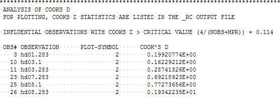
24 Back to: EVALUATING PARAMETER ESTIMATION OUTPUT from Residual_analysis fn#resan _rc _r Cook sd large values indicate oservations that most influence all estimated parameter values DFBetaS large values indicate oservations important to individual parameters Do you understand why the flow oservation is so important? What would you e ale to say aout the parameter values without that oservation? A typical _rc 24

25 A typical _r Typical #resan results 25

26 EVALUATING PARAMETERIZATION High parameter correlations calls for either Additional data that will reak the correlations Or Reparameterization Barring the availaility of additional data, consider reparameterization eg USING DERIVED_PARAMETERS Block As an example you could define rch2=05*rch1 and rch3=01*rch1 However, notice that the true values do not have those ratios To evaluate if correlations are too high try starting from different values USE PARAMETER_VALUES Block If results are the same (parameter values fall within one standard deviation of those determined with different starting values) correlation is not an issue Thus parameters are eing independently estimated Overview of UCODE & Associated Codes Modes that can e accomplished: Forward Process Model run with Residuals Conduct Sensitivity Analysis Estimate Optimal Parameter values and associated linear uncertainty Evaluate quality of the model Estimate values of Predictions and associated linear uncertainty Evaluate model linearity Evaluate NonLinear uncertainty associated with estimates of parameter values and predicted values Auxiliary: Investigate Ojective Function See UCODE Manual Chapter 1 for overview and description of manual contents 26

27 When prediction=yes, UCODE calculates predictions and sensitivities (if sensitivities=yes) of the model parameters to those predicted values for the purpose of calculating 95-percent linear confidence and prediction intervals on the predictions IN PREDICTION MODE WE CHANGE THE PROCESS MODEL TO THE PREDICTIVE CONDITIONS We will get oth CONFIDENCE INTERVALS and PREDICTION INTERVALS ON PREDICTED VALUES CONFIDENCE INTERVALS are ased on var-cov of parameters, reflecting certainty associated with the parameters PREDICTION INTERVALS are ased on var-cov of parameters AND the measurement error reflecting our aility to measure the predicted value 3 ALTERNATIVE METHODS OF CALCULATION OF INTERVALS for oth CONFIDENCE INTERVALS AND PREDICTION INTERVALS on PREDICTIONS Appropriate method depends on # of predictions jointly considered 1) INDIVIDUAL INTERVALS 2) SIMULTANEOUS INTERVALS - more than one interval 3) SIMULTANEOUS INTERVALS - undefined numer of intervals (eg drawdown over an area must e limited to a given magnitude, ut the location of the maximum drawdown cannot e determined a priori) Only the critical values differ and are otained from one of: Student-t Distriution Bonferroni-t Distriution Scheffe (ased on the F-distriution) i i UCODE tests for the appropriate method, then prints intervals for Individual and Both Simultaneous Intervals Of these 3, the user selects the interval appropriate for their question 27

28 INDIVIDUAL CONFIDENCE INTERVALS Sensitivity of the simulated equivalent of the prediction to the parameters NP NP z s z = V( ij ) z i=1 j=1 j i 1 2 Element ij of the variance/covariance matrix SIMULTANEOUS CONFIDENCE INTERVALS Two Methods: Bonferroni & Scheffe Both conservative with respect to significance level Both are calculated y UCODE and the smaller is used Bonferroni: Scheffe: 28

29 PREDICTION INTERVALS are roader than confidence intervals ecause they include the proaility that the MEASURED value will fall into the interval Calculations are the same as for confidence intervals, however the standard deviation is increased to reflect the measurement error as follows: EVALUATE PREDICTIVE UNCERTAINTY using OPTIMAL PARAMETER VALUES with UCODE Develop a predictive MODLFOW Model Import to ModelMate as per instructions in PDF file Run UCODE with prediction=yes, first to e sure all is functioning correctly Then with sensitivity=yes UCODE calculates the sensitivity of the predictions to the parameters at the optimal values linear_uncertainty is executed in that folder with the ucode root file name as input, eg C:\WRDAPP\UCODE_2005\in\linear_uncertaintyexe ep_ucode NOTE IF you use different root names for caliration and prediction ucode runs you must use ucode 1020 or later for the linear uncertainty run ALWAYS USE THE LATEST VERSION OF ALL MODELING CODES 29

30 This ucode prediction execution does not overwrite previously created UCODE output files It produces additional files #upred _p _pv _dmp _spu _sppp _sppr _spsp _spsr The linear_uncertainty execution produces #linunc and _linp You can view the results in GW_Chart DUE TODAYCOMPUTER FILES AND QUESTIONS for Assgn#6 Assignment # 6 Steady State Model Caliration: Calirate your model If you want to conduct a transient caliration, talk with me first Perform caliration using UCODE Be sure your report addresses gloal, graphical, and spatial measures of error as well as common sense Consider more than one conceptual model and compare the results Rememer to make a prediction with your calirated models and evaluate confidence in your prediction Be sure to save your files ecause you will want to use them later in the semester Suggested Caliration Report Outline Title Introduction descrie the system to e calirated (use portions of your previous report as appropriate) Oservations to e matched in caliration type of oservations locations of oservations oserved values uncertainty associated with oservations explain specifically what the oservation will e matched to in the model Caliration Procedure Evaluation of caliration residuals parameter values quality of calirated model Calirated model results Predictions Uncertainty associated with predictions Prolems encountered, if any Comparison with uncalirated model results Assessment of future work needed, if appropriate Summary/Conclusions References sumit the paper as hard copy and include it in your zip file of model input and output sumit the model files (input and output for oth simulations) in a zip file laeled: ASSGN6_LASTNAMEZIP 30