Multiple Regression: Chapter 13. July 24, 2015

Transcription

1 Multiple Regression: Chapter 13 July 24, 2015

2 Multiple Regression (MR) Response Variable: Y - only one response variable (quantitative) Several Predictor Variables: X 1, X 2, X 3,..., X p (p = # predictors) Note: the predictors can be quantitative, categorical, quadratic term, interaction term

3 Concentrate on: Reading computer output Interpreting coefficients for each Predictor Determining which order to test in picking the simplest model that does a good job for predicting Y

4 The Basic of MR Model: Y = α + β 1 X 1 + β 2 X β p X p + ɛ ( predictors: X 1, X 2,..., X p, # predictors: p) Assumptions: ɛ iid N(0, σ) Parameters: coefficients: β 1, β 2,..., β p constant: α

5 Reading the computer output: 1. Fitted Equation: ŷ = a + b 1 X 1 + b 2 X b p X p 2. ANOVA Test: H 0 : β 1 = β 2 =... = β p = 0 (nothing good in model) H a : at least one β i 0 (something good) Test Statistic: F = MSR MSE ANOVA table for regression Source df SS M S F P-value Regression p SSReg MSR MSR (from F table with MSE Error n p 1 SSE MSE df num, df denom ) Total n 1 SST

6 3. t test for Individual Predictors: H 0 : β i = 0 vs H a : β i 0 b Test Statistic: t = i 0 standard error of b i p-value computed from t-table with df= n p 1 (error) Interpretation: if p-value small, reject H 0 - conclude that predictor X i is a GOOD predictor of Y (X i provides significance information about Y ) AFTER all other predictors in the model are accounted for

7 Important Issues in Multiple Regression Don t just add predictors to the model - think! For p = n we have oversaturated model with R 2 = 100% (not useful to predict for larger populations, but only for this particular dataset) adjusted R 2 only increases if the new predictor added to the model is good, whereas R 2 goes up or stays the same even if the new predictors are bad Remember to look at p-values for each predictor.

8 Multicollinearity: when several predictors are correlated with each other, then the ANOVA p-value may be small even if all the individual t-test p-values are large. Correlated predictors give overlapping or redundant information. (Don t throw out all the predictors but take them out of model slowly) Sample size should be at least 5 to 20 times bigger than the number of predictors

9 Example: The following is the dataset on Blood Alcohol Content (BAC) and the Number of Beers consumed (NOB) with two more variables Weight and Sex. We fit different regression models and compare the output. BAC NOB Weight Sex M 1 F f f f m m f f m f m f m f m m m 1 0

10 Regression Analysis: BAC versus NOB The regression equation is BAC = NOB Predictor Coef SE Coef T P Constant NOB S = R-Sq = 80.0% R-Sq(adj) = 78.6% Analysis of Variance Source DF SS MS F P Regression Residual Error Total

11 Regression Analysis: BAC versus NOB, M_1 The regression equation is BAC = NOB M_1 Predictor Coef SE Coef T P Constant NOB M_ S = R-Sq = 85.3% R-Sq(adj) = 83.1% Analysis of Variance Source DF SS MS F P Regression Residual Error Total

12 Regression with Dummy Variables: Dummy Variable: Categorical variable coded as 0 or 1 0 if female Example: Let X 2 =Gender = 1 if male (baseline group has zero for dummy variable) Model (no interaction): Y = α + β 1 X 1 + β 2 X 2 + ɛ Note: This model gives two lines - one for females and one for males with same slope but different intercepts. F (X 2 = 0) Y = α + β 1 X 1 + ɛ M (X 2 = 1) Y = (α + β 2 ) + β 1 X 1 + ɛ

13 Interpret Coefficients: α β 1 β 2 y-intercept for baseline group (F) slope for both groups change in intercept for males compared to females

14 Regression Analysis: BAC versus NOB, Weight The regression equation is BAC = NOB Weight Predictor Coef SE Coef T P Constant NOB Weight S = R-Sq = 95.2% R-Sq(adj) = 94.4% Analysis of Variance Source DF SS MS F P Regression Residual Error Total

15 Regression Analysis: BAC versus NOB, Weight, M_1 The regression equation is BAC = NOB Weight M_1 Predictor Coef SE Coef T P Constant NOB Weight M_ S = R-Sq = 95.3% R-Sq(adj) = 94.1% Analysis of Variance Source DF SS MS F P Regression Residual Error Total

16 Question: What if gender coded the other way? Regression Analysis: BAC versus NOB, Weight, F_1 The regression equation is BAC = NOB Weight F_1 Predictor Coef SE Coef T P Constant NOB Weight F_ S = R-Sq = 95.3% R-Sq(adj) = 94.1% Analysis of Variance Source DF SS MS F P Regression Residual Error Total

17 Interaction model: (with dummy) Y = α + β 1 X 1 + β 2 X 2 + β 3 X 1 X 2 + ɛ Note: This model gives two lines - one for females and one for males with different slopes and different intercepts. F (X 2 = 0) Y = α +β 1 X 1 +ɛ M (X 2 = 1) Y = (α + β 2 ) +(β 1 + β 3 )X 1 +ɛ Interpret Coefficients: α β 1 β 2 β 3 y-intercept for baseline group (F) slope for baseline group (F) change in intercept for males compared to females change in slope for males compared to females

18 Regression Analysis: BAC versus NOB, Weight, M_1, Weight*M_1 The regression equation is BAC = NOB Weight M_ Weight*M_1 Predictor Coef SE Coef T P Constant NOB Weight M_ Weight*M_ S = R-Sq = 95.5% R-Sq(adj) = 93.9% Analysis of Variance Source DF SS MS F P Regression Residual Error Total

19 What if we had 3 groups? Suppose we want to predict BAC from NOB and Race: white, black, hispanic Need 2 dummy variables for 3 categories. Let X 2 = 1 if black 0 otherwise, X 3 = 1 if hispanic 0 otherwise Note: Race = White, is the baseline zero for both dummy variables.

20 No Interaction model with 2 Dummies: Y = α + β 1 X 1 + β 2 X 2 + β 3 X 3 + ɛ which gives the following 3 equations: X 2 = 0, X 3 = 0 (W): X 2 = 1, X 3 = 0 (B): X 2 = 0, X 3 = 1 (H): Y = α + β 1 X 1 + ɛ Y = (α + β 2 ) + β 1 X 1 + ɛ Y = (α + β 3 ) + β 1 X 1 + ɛ Interpret Coefficients: α β 1 β 2 β 3 intercept for baseline group (W) slope for all 3 groups change in intercept for blacks compared to whites change in intercept for hispanic compared to whites

21 Interaction Model: add interactions between the quantitative variable (X 1 ) and the dummy variables (X 2, X 3 ) Y = α+β 1 X 1 +β 2 X 2 +β 3 X 3 +β 4 X 1 X 2 +β 5 X 1 X 3 +ɛ which gives the following 3 equations: X 2 = 0, X 3 = 0 (W): X 2 = 1, X 3 = 0 (B): X 2 = 0, X 3 = 1 (H): Y = α + β 1 X 1 + ɛ Y = (α + β 2 ) + (β 1 + β 4 )X 1 + ɛ Y = (α + β 3 ) + (β 1 + β 5 )X 1 + ɛ Interpret Coefficients: α intercept for baseline group (W) β 1 slope for W β 2 change in intercept for B compared to W β 3 change in intercept for H compared to W β 4 change in slope for B compared to W change in slope for H compared to W β 5

22 In regression, if we have only one categorical predictor, REGRESSION ONE-WAY ANOVA Revisit the ONE-WAY ANOVA Example: Compare average weight loss for three diets. Data: Weight loss under 3 diets low FAT low CAL low CARB

23 ANOVA results (output): One-way ANOVA: lowfat, lowcal, lowcarb Source DF SS MS F P Factor Error Total S = R-Sq = 66.79% R-Sq(adj) = 59.41% Individual 95% CIs For Mean Based on Pooled StDev Level N Mean StDev lowfat ( * ) lowcal ( * ) lowcarb ( * ) Pooled StDev = 2.598

24 Now, let s set up the problem as regression with dummy variables. Y = weight loss (response) Let X 1 = 1 if lowcal 0 otherwise, X 2 = 1 if lowcarb 0 otherwise Model: Y = α + β 1 X 1 + β 2 X 2 + ɛ Interpret Coefficients: α β 1 β 2 intercept for baseline group (lowfat) change in intercept for lowcal compared to lowfat change in intercept for lowcarb compared to lowfat

25 REGRESSION results (output): Regression Analysis: Y versus x1, x2 The regression equation is Y = x x2 Predictor Coef SE Coef T P Constant x x S = R-Sq = 66.8% R-Sq(adj) = 59.4% Analysis of Variance Source DF SS MS F P Regression Residual Error Total

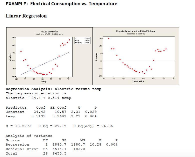
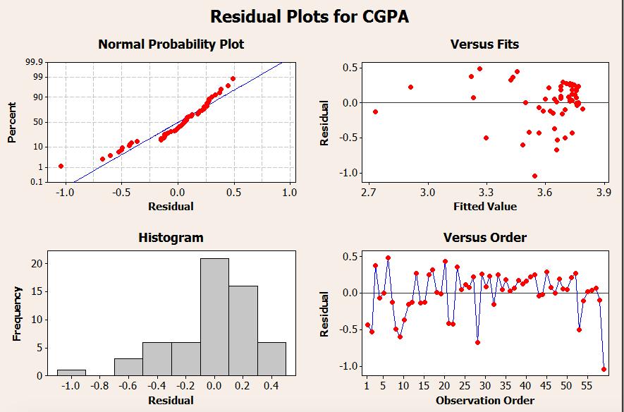
26 More about RESIDUALS: Plot of RESIDUALS vs FITTED value will exaggerate any pattern present in data other than linear trend. How to judge non constant variance in response from residual vs fitted plot? (example in class) Recall: residuals = y ŷ (i.e. linear trend is removed from the model) any pattern (or trend) still present in residual vs fitted value plot suggests that the linear regression was not enough. Need to add quadratic (or other polynomial) terms in the equation (examples in class)

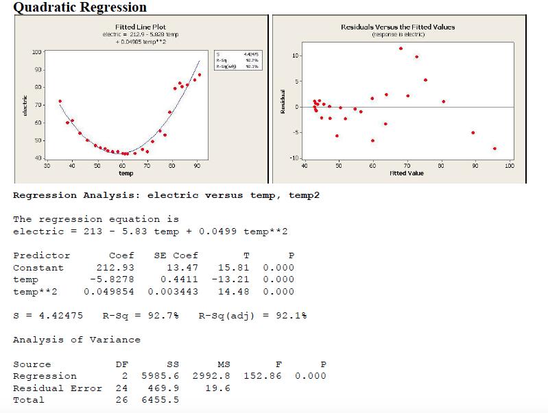
27 QUADRATIC REGRESSION Model: Y = α + β 1 X + β 2 X 2 + ɛ, note that p = 2 predictors (X, X 2 ) Assumptions: ɛ iid N(0, σ) Fitted Equation (output): ŷ = a + b 1 X + b 2 X 2 Interpret Coefficient: Only interpret the coefficient for the quadratic term. Is β 2 significantly different from zero? if yes - keep quadratic term - look for sign of b 2 (determines whether curvature opens up or down) if no - throw X 2 out - do SLR

28

29

30 Example: Suppose we are interested in predicting the GPA of students in college (CGPA) using 16 different predictor variables. Data were collected from a random sample of 59 college students. What is the response variable in this problem? What are the values of n and p? What are Ho and Ha that you can test using the ANOVA table? What is your decision, based on the following ANOVA table? What is your conclusion?

31 Regression Analysis: CGPA versus Height, Gender,... The regression equation is CGPA = Height Gender Haircut Job Studytime Smokecig Dated HSGPA HomeDist BrowseInternet WatchTV Exercise ReadNewsP Vegan PoliticalDegree PoliticalAff Predictor Coef SE Coef T P Constant Height Gender Haircut Job Studytime Smokecig Dated HSGPA HomeDist BrowseInternet WatchTV Exercise ReadNewsP Vegan PoliticalDegree PoliticalAff

32 S = R-Sq = 43.2% R-Sq(adj) = 21.5% Analysis of Variance Source DF SS MS F P Regression Residual Error Total

33 Best Subsets Regression: CGPA versus Height, Gender,... Response is CGPA B o r l o i P w t o s i l S e R c i t S H I E e a t H u m o n W x a l i H G a d o m t a e d D c e e i y k D H e e t r N V e a i n r t e a S D r c c e e g l g d c J i c t G i n h i w g r A Mallows h e u o m i e P s e T s s a e f Vars R-Sq R-Sq(adj) Cp S t r t b e g d A t t V e P n e f X X X X X X X X X X X X X X X X X X X X X X X X X X X X X X

34 X X X X X X X X X X X X X X X X X X X X X X X X X X X X X X X X X X X X X X X X X X X X X X X X X X X X X X X X X X X X X X X X X X X X X X X X X X X X X X X X X X X X X X X X X X X X X X X X X X X X X X X X X X X X X X X X X X X X X X X X X X X X X X X X X X X X X X X X X X X X X X X X X X X X X X X X X X X X X X X X X X X X X X X X X X X X X X X X X X X X X X X X X X X X X X X X X X X X X X X X X X X X X X X X X X X X X X X X X X X X X X X X X X

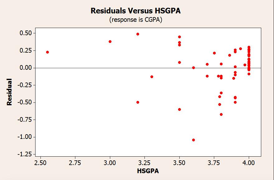
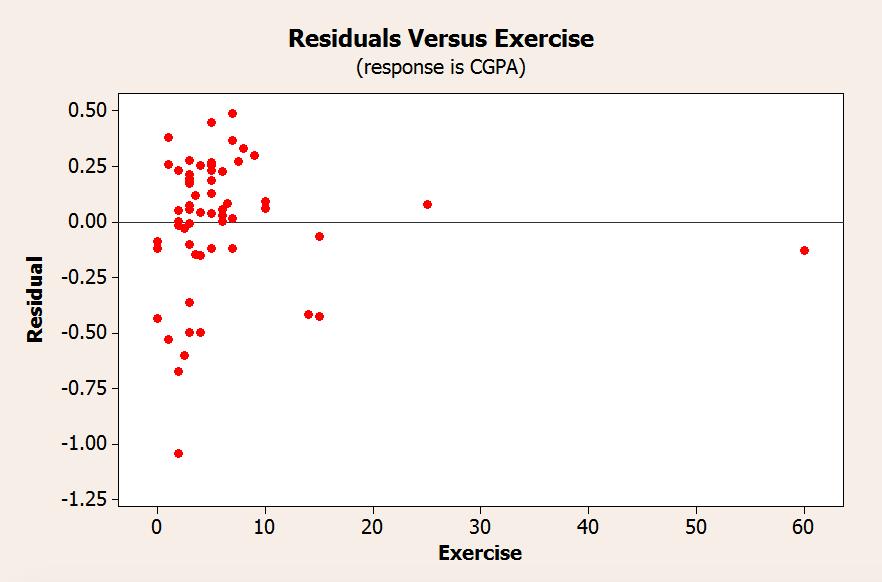
35 Regression Analysis: CGPA versus HSGPA, Exercise The regression equation is CGPA = HSGPA Exercise Predictor Coef SE Coef T P Constant HSGPA Exercise S = R-Sq = 31.6% R-Sq(adj) = 29.2% Analysis of Variance Source DF SS MS F P Regression Residual Error Total

36

37 LOGISTIC REGRESSION Y = Categorical Response (Yes/No) or Binary Response (1 or 0) Example: Predict the probability that a person pay bills on time based on past credit history, income, employment, age, etc.. Example: Predict the probability that a person gets lung cancer based on smoking, family history, asthma, age, gender, race, eating habit, exercise habit, etc..

38 Logistic Regression Model: (with 1 predictor variable) p = exp(α + βx) 1 + exp(α + βx) Example: Whether a person has travel credit card. X = annual income (in thousand euros), y = (partial dataset..) income y if yes 0 if no

39 Link Function: Logit Response Information Variable Value Count y 1 31 (Event) 0 69 Total 100 Logistic Regression Table Predictor Coef SE Coef Z P Constant income

40 Interpretations: Annual income is a good predictor of probability of having a travel credit card the probability of having a travel credit card increases (because of the positive sign of the coefficient) with higher annual income.

41 Prediction Equation: ˆp = exp( X) 1 + exp( X) i.e. a = 3.52, b = predict the probability that person with annual income 12K (euros) has a travel credit card (answer: ˆp = 0.09) predict the probability that person with annual income 65K (euros) has a travel credit card (answer: ˆp = 0.97) the probability of having a travel credit card is 50% when X = a b = = (why?)

42 Multiple Logistic Regression: Example: Predict Marijuana use (Y/N) based on Alcohol use (Y/N) and cigarette smoking (Y/N) for HS seniors. Data: 2276 HS seniors in non-urban area outside Dayton, Ohio. Marijuana Cigarette Alcohol Frequency

43 Binary Logistic Regression: Marijuana versus Alcohol, Cigarette Link Function: Logit Response Information Variable Value Count Marijuana (Event) Total 2276 Frequency: Frequency Logistic Regression Table Predictor Coef SE Coef Z P Constant Alcohol Cigarette

44 Predict probability of using Marijuana if Alcohol use = Yes and Cigarette smoking = Yes ˆp = exp( ) 1 + exp( ) = Alcohol use = No and Cigarette smoking = Yes ˆp = exp( ) 1 + exp( ) = 0.079