Vmax DR = (2.1) Vmin. max. min

Transcription

1 Seismographic Systems It is common to separate seismographic systems into seismographs and strong-motion accelerographs. Seismographs have generally been developed by geophysicists and seismographs are typically designed to record ground motions that are far too small to be felt. Strong-motion accelerographs have usually been designed by earthquake engineers to record the ground acceleration during severe earthquake shaking. In actuality, though, there is nothing fundamentally different in the physics of these two systems. Seismographs (including strong-motion accelerometers) consist of (at least) a sensing unit and a recording unit. I will begin by discussing the recording system. Current stateof-the-art is to record output voltages from a seismometer (the sensing system) with a digital data logger, which typically consists of an analog to digital converter (ADC) and some type of digital computer for processing, storage, and communications. Dynamic Range The most critical specification of a data logger is its dynamic range, which is defined as the ratio of the largest on-scale voltage V max divided by the smallest resolvable voltage V min. That is, Vmax DR = (.1) V Traditionally, dynamic range is given in the somewhat obscure units of decibels db (a tenth of a Bell). This nomenclature was originated with measuring the relative intensity of sound, which is proportional to the power of acoustic waves. Bells are a base 10 logarithmic measure of energy per unit time, and 1 Bell corresponds to a factor of 10 increase in energy per unit time. However, most of our discussions concern the amplitude of some signal as opposed to its power. Since power is proportional to the square of the amplitude, a factor of 10 in amplitude corresponds to Bells or 0dB. Therefore we can define dynamic range in units of db as V max DR = 0 log db (.) Vmin The dynamic range of a digitizer is typically determined by the number of bits that it uses to characterize voltage. Each bit represents a factor of in dynamic range, so the #bits dynamic range is. Since log = 0.301, the dynamic range in db is #bits times 6.0. Early digitizers were typically 8-bit or 1-bit units. 16-bit units were common by the mid 1980 s, and 0-bit or 4-bit units had become the standard by the mid 1990 s. Some examples of dynamic range are given in Table.1. min -1

2 Table.1 #bits Dynamic Range DR in db , , ,048, ,777, Paper or film recording devices were the most common system prior to introduction of digital systems. These older analog systems typically had a dynamic range of 50 to 60 db, depending on how well the trace could be measured. As we shall see later, the total dynamic range of motions encountered in the Earth is on the order of 00 db, and current digitizers do not come close to having the dynamic range to record both the strongest motions in earthquakes and the smallest motions that occur at quiet sites. Most electro-mechanical seismometers have an effective dynamic range that is about 100 db, which is much larger than the range of optical recording systems. However, electronic feedback seismometers (described below) typically have dynamic ranges of about 140 db. Seismometers Seismometers are the sensors that produce the signal to be recorded. Modern seismometers produce some voltage that is related to the ground motion by the instrument response. The earliest seismometers (circa 1900) consisted of a mass, a spring, and sometimes a damper. The mass was usually very large since its motion was typically measured by a series of levers that caused a needle stylus to move over a rotating drum covered with smoked paper. Thus it was necessary for the small motions of the ground to cause enough momentum in the mass to overcome the friction of the recording system. In 19, Harry Wood (a seismologist) and John Anderson (an astronomer) collaborated to build a simple system known as the Wood-Anderson torsion seismometer. They developed a system that illuminated a mirror on a mass suspended by a vertical wire that served as a torsion spring. When the ground moved horizontally, the wire would twist, causing a deflection of the reflected light. The reflected light was focused onto a rotating drum covered with photographic paper. The motion of the mass was damped electromagnetically. The Wood Anderson has undamped natural period of 0.8 s, it s gain is,800, and its damping is 70% of critical. Several dozen Wood-Anderson seismometers were operated in southern California until about This system was the standard that was used by Richter in the definition of earthquake magnitude in the 1930 s. The response of this instrument is that of a simple single degree-of-freedom oscillator. Many strong-motion accelerographs were also simple optical SDOF s. More than 10,000 SMA-1 series of accelerographs were manufactured by Kinemetrics in Pasadena from the -

3 late 1960 s to the mid 1990 s. This instrument also has a mirror that deflects in torsion. It s natural frequency is about 30 Hz and it also 70% damped. A sketch of this instrument is shown in Figure.1. A frequencies lower than 30 Hz, the records from this instrument are proportional to ground acceleration. These instruments record on 70 mm film and they only record when triggered by vertical accelerations that exceed about 1% g. The clip level on an SMA1 is about 1.5 g. When the frequency of the signal exceeds 15 Hz, it is necessary to deconvolve the instrument response to obtain true ground acceleration from this instrument. Figure. shows a schematic of another common strong motion accelerometer (SMAC) used in Japan from the 1960 s through the 1980 s. This is a purely mechanical instrument with air damping. Unfortunately, static friction in the system made this a poor system for recording motions at periods exceeding seconds. Figure.1 Schematic of the mechanics of an SMA-1 strong motion accelerometer. -3

4 Figure.. Schematic of a Japanese SMAC strong motion acclerograph. Table.1 gives the instrument constants of a number of strong-motion seismographs. Table.1-4

5 Beginning in the 1910, seismometers with electromagnetic pickups were developed by Galitzen. Currents generated by the seismometer were used to drive a galvanometer that that deflected a beam of light. A number of different types of these instruments became popular in the 1930 s. These instruments gave new flexibility since the signals could electronically amplified and filtered. Velocity transducers are the most common type of pickup and they typically consist of a magnetized mass that moves through a conducting coil. The voltage generated in the coil is proportional to the velocity of the mass with respect to the coil, and hence the term, velocity transducer. Benioff short-period seismometers with a 1-second free period, 70% damping, and velocity transducers were important standards in seismology. By the 1970 s more compact 1-second velocity seismometers were manufactured in large numbers for use in exploring for petroleum. Over a thousand L4-C (Mark Products, Inc) 1-second seismometers were employed by regional seismic U.S. networks from the 1970 s through the 1990 s. The electrical output from these seismometers has been recorded in a number of ways. In many important seismographic systems, the electrical current from the seismometer was used to drive galvanometers. These galvanometers consisted of a mirror suspended on a torsion wire. Deflection of the mirror was measured photographically as in other direct seismometers. The galvanometer was itself a linear SDOF whose forcing was the output from the seismometer. The galvanometer/seismometer system actually constitutes linearly coupled oscillators. Therefore, the response of these galvanometer seismometer systems is approximately given by. x t + βx t + ω x t = u t (.3) () ( ) ( ) ( ) 0 ( ) Cx( t) V t = (.4) () + β ( ) + ω ( ) = ( ) y t y t y t DV t (.5) G G where x(t) and y(t) correspond to the motion of the seismometer and galvanometer masses, respectively, C and D are constants, V( t) is voltage, βg and ω G are the damping and free period of the galvanometer. Note that the driving term in the second equation is not a nd derivative with respect to time. Since the damping of both systems was 70% of critical, and since older seismometer masses were quite large, the feedback from the motion of the galvanometer back into the seismometer was minimized. Therefore we can approximately solve this problem as if the solution to equation (.3) is used as the input to equation (.5). As was the case for the simple SDOF, we can write the solution for these equations as a convolutions with the Green s functions of the seismometer G(t) and the galvanometer G G (t). -5

6 where and () = ( ) ( ) y t G t V t G G d = GG () t D CG() t u() t dt = CDG t G t u t () () () 1 βt () = sin ( ω0 β ) G t e t ω β 0 1 βgt () = sin ( ωg βg ) GG t e t ω β G G (.6) (.7) (.8) The dynamic range of these electromagnetic seismometers is typically in the range of 80 to 100 db. This is far greater than the range of the film or paper systems that were used to record the data from them. Just as before, we can take the Fourier transform of (.6) to obtain where 3 ( ω) = ( ω) ( ω)( ω ) ( ω) y CDG G i u (.9) G 1 G ( ω ) = ω0 ω + iωβ (.10) 1 G G ( ω ) = ω ω + iωβ (.11) G G Table 4.1 lists some instrument constants for several seismometer systems. All of these systems are from the early 1900 s, except for the WWSSN LP, which was operated as a standard world-wide network from the 1960 s to the 1980 s. -6

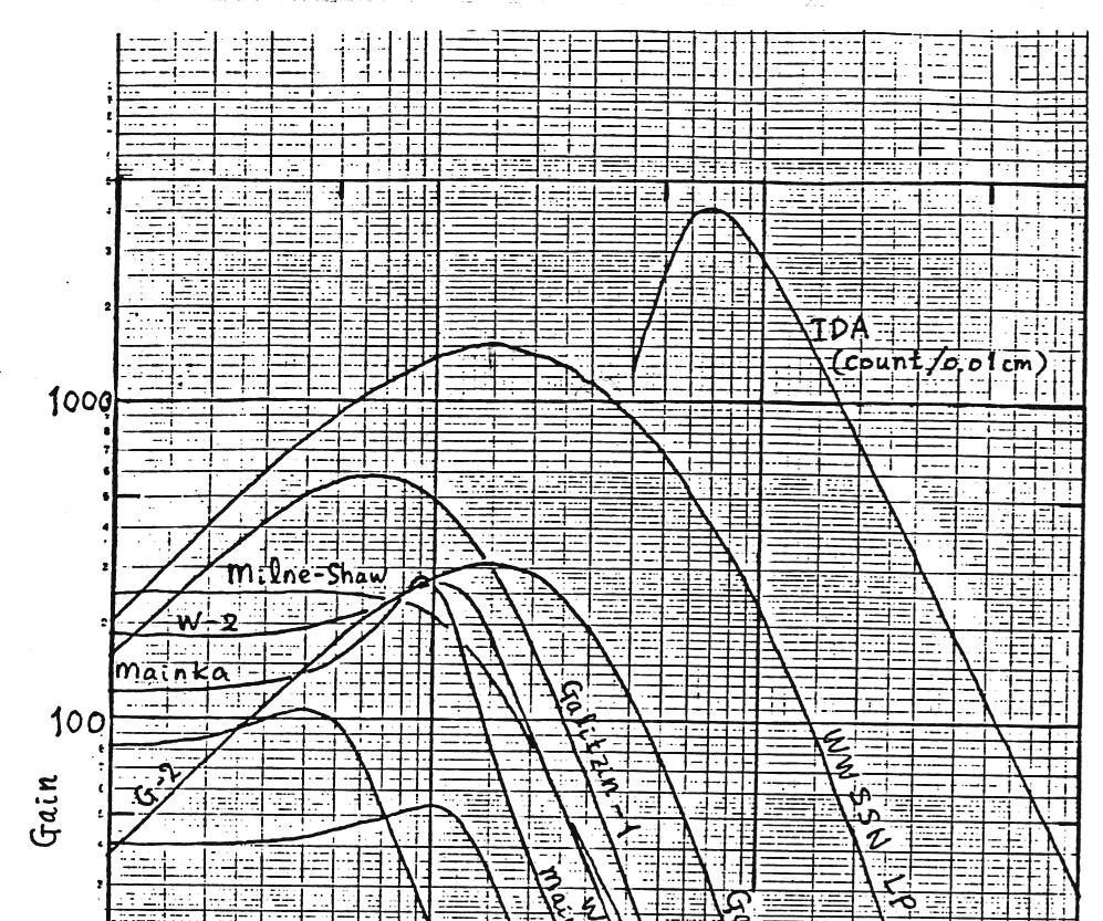
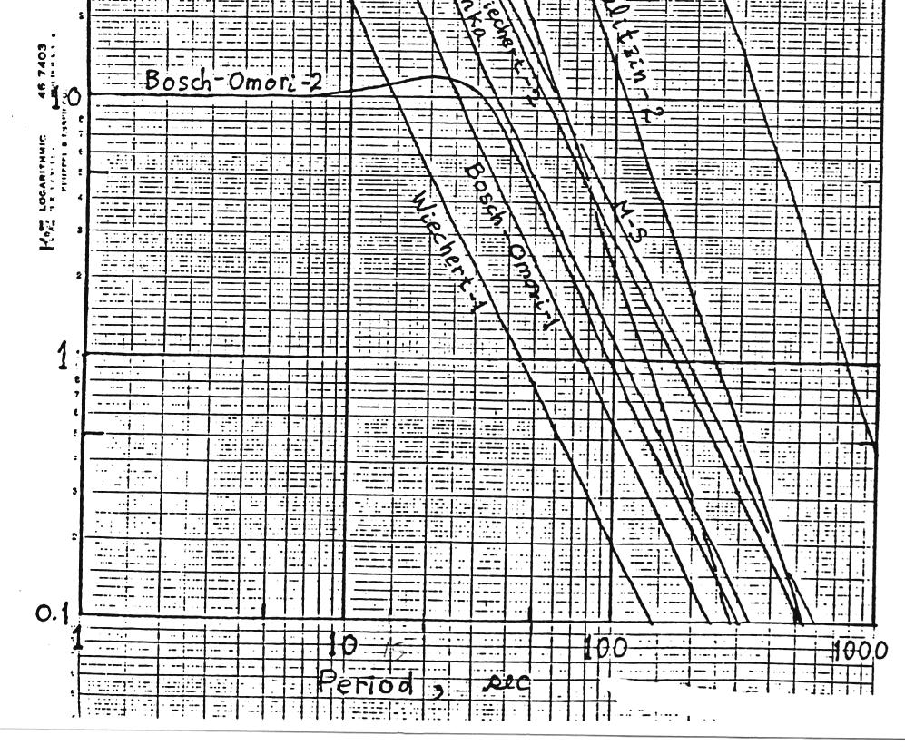
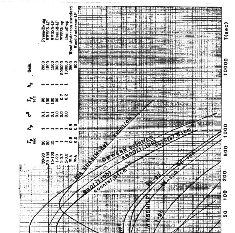
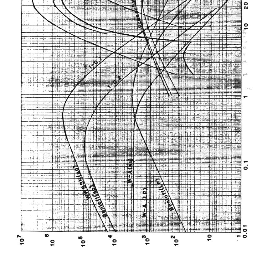
7 π The ground displacement amplification response as a function of period T = is ω shown in Figure.3. Figure.4 shows a similar plot for a number of important seismographic systems, many of which were operated at the Seismological Laboratory of Caltech. -7

8 -8

9 -9

10 Poles and Zeros We can rewrite the frequency domain response of our seismometer/galvanometer system (.9) in the following way y( t) = R( t) u( t) (.1) where R(t) is the displacement response of the system given by d R() t = CDG 3 () t GG () t dt (.13) This can be written in the frequency domain as y ω = R ω u t (.14) where where and R = ( ω ) ( ) ( ) () 3 CD( iω ) = ( ω0 ω + iωβ )( ωg ω + iωβg) 3 CD( iω ) ( ω ω0 iωβ)( ω ωg iωβg) 3 ( iω ) ( i ) ( i ) = CD ω β + β ω0 ω βg + βg ω G = icd ( ω z1)( ω z)( ω z3) ( ω p )( ω p )( ω p )( ω p ) p p p (.15) z1 = z = z3 = 0 (.16) = iβ ω β (.17) 0 = iβ + ω β (.18) 0 = iβ ω β G (.19) 3 G G p4 = iβg + ωg β G (.0) The p j and z i are called the poles and zeros of this system, and together with the station gain, -icd, they define the response of the system. Unfortunately, there is always confusion about conventions used in transforms. The common convention for poles and zeros is defined by the Standard for Exchange of Earthquake Data (SEED). This standard is described in the SEED user s manual that can be found at The standard is based on Laplace transforms as opposed to Fourier transforms. These two transforms are very similar except that the poles are zeros are defined in terms of the Laplace transform variable s = iω. Denoting the poles and zeros by P i and Z i, we can rewrite (.15) as -10

11 where and ( ω ) ( s Z1)( s Z)( s Z3) ( )( )( )( ) R = CD s P s P s P s P (.1) Z1 = Z = Z3 = 0 (.) P = ip = + (.3) P P 1 1 β β ω 0 = ip = (.4) β β ω 0 = ip = β + β ω G (.5) 3 3 G G 4 4 βg βg ω P = ip = G (.6) In fact, any complex transfer function that can be written in the form n n 1 anω + an 1ω a T ( ω ) = 0 (.7) l l 1 blω + bl 1ω b0 can also be written in the form T ( ω ) a = b n i= 1 ( ω z ) l ( ω pj ) j= 1 i (.8) The convention of using poles and zeros is especially useful in systems that can be described as a series of convolutions. Since these convolutions can be written as a series of multiplications in the frequency domain, a system can be described by compiling the set of all of the poles and zeros that correspond to each of the functions that are convolved to form the transfer function. If an additional filter or device is added to the system (and if its effect is that of a convolution), then the poles and zeros of that device are simply added to the set. Broad-Band Seismometers It is worth inspecting Figure.4 to see that most seismographic systems were designed to have high magnification in either a short-period band (about 1 second) or a long-period band (about 0 seconds). This was accomplished by using short-period galvanometers together with short-period seismometers to make a short period seismograph, or by combining a long-period galvanometer with a long-period seismometer to make a longperiod seismograph. However, it was possible to use a short-period seismometer with a long-period galvanometer to make a system which records over a broad range of frequencies. One such instrument was the Benioff 1-90, which had a 1-second velocity transducer seismometer driving a 90-second galvanometer. The response of this instrument (see Figure.4) is approximately flat to velocity between 1 and 90 seconds; hence it records velocity over a broad frequency range. Notice that the amplification of the 1-90 is much less than that of either the short- or long-period systems. This is because there are microseisms, which are relatively large -11

12 amplitude waves continuously, excited by water waves in the ocean at periods between 6 and 1 seconds. There was not much point in making a high-magnification broad-band system since it would fill the seismogram with quasi-harmonic microseisms. The presence of microseismic noise at virtually all stations meant that seismograph designers who wished to detect and locate frequent small-magnitude earthquakes were forced to design either long- or short-period instruments. Simple optical seismometers (Wood-Anderson, SMA-1 accelerograph) also respond over a broader frequency band, but they have a relatively small overall amplification of signals. Furthermore, their response is flat to acceleration at periods longer than their natural frequency. This means that they are quite insensitive to long-period ground displacements when compared to a seismograph that whose response is flat to velocity. Figure.5 shows that amplitude for many different wave types as a function of frequency. The vertical axis is the log of the max amplitude of a seismogram after filtering with a 1-octave wide bandpass filter. The curves labeled maximum and minimum correspond to the background noise level recorded at worldwide seismographic stations. The minimum curve was recorded at a site in Lajitas, Texas. There is really no maximum curve, since one can always find sites with high background noise. It actually represents the noise encountered on ocean island stations where ocean wave generated noise is high. The various lines shown for different earthquake situations show approximate median amplitudes for earthquakes recorded at approximately 10 km, 100 km, and 3000 km from earthquakes of different magnitudes. You can see that there are more than 00 db in amplitude difference (10,000,000,000 to 1) between the ambient ground noise and the maximum ground accelerations at seismically quiet sites. The stippled regions show the on-scale range of both an SMA-1 strong motion accelerograph and a typical short-period seismographic channel from a regional seismographic network with analog telemetry (frequency modulated, FM). Almost 1,600 of these short period seismographs were operating in the United States in the 1980 s. These stations were designed to operate at maximum magnification to detect the smallest earthquakes that created motions just larger than the ambient ground motions. Although these stations were well suited for detecting ground motions, they were not well suited for recording them. That is, many earthquake ground motions were too large for the range of the system and they caused clipping. Some seismological observatories operated a wide variety of seismographs that operated in different amplitude and frequency bands. The Pasadena station routinely recorded several dozen seismograms each day in order to obtain a more or less complete record of ground motion over this vast range of amplitude and frequency. -1

13 Figure.5 Notice that the spectra of ground accelerations from strong motion records of large earthquakes are relatively flat in the frequency band from 0.3 Hz to 5 Hz. Since the recording system of early strong motion accelerographs was less than 60 db, it was a -13

14 good choice to record ground acceleration since that was the best way to recover motion in the frequency band from 0.1 Hz to 10 Hz. In the 1980 s seismic instrumentation was revolutionized by the development of forcefeedback seismometers. These systems are similar to standard seismometers, but they usually have a displacement transducer to measure the motion of the seismometer mass. In addition, they add an electromagnetic forcing system that has the role of minimizing the motion of the mass with respect to the seismometer case. The force necessary to keep the mass stationary is simply the ground acceleration. The essential feature of these systems is that the dynamic range of the instrument is dictated by the dynamic range of the electronic feedback system, and not by the dynamic range of the mechanical seismometer. This essential addition allows modern feedback seismometers to often achieve 140 db dynamic ranges (a factor of 100 times greater than the dynamic range of mechanical systems). The electronic feedback system can also be designed to provide the desired instrument response. STS-1 seismometers manufactured by Streckeisen A.G. in Switzerland are considered a standard of excellence for feedback seismometers. They have a mechanical natural period of about 1 Hz that is extended to Hz (360 seconds) by the feedback system. Their electronic feedback system is designed to provide an instrument response that is flat to velocity from 360 seconds to 8 Hz. In essence they have a response that is identical to an SDOF with a 360 second natural period and a velocity transducer. The range of amplitudes and frequencies that can be recorded by an STS-1 are shown in Figure.5. Notice that microseismic noise in the. Hz to.1 Hz band is several orders of magnitude larger than the minimum motion resolved from an STS-1. Thus, it is necessary to filter in this frequency band if one wants to see small motions in either shorter or longer periods. Such filtering was not particularly feasible when STS-1 s were recorded with older systems with limited dynamic range. The development of 4-bit recording systems with dynamic ranges of 140 db that matched that of the seismometer was the other important development that revolutionized seismographic systems in the 1990 s. A number of other important feedback seismometers have been developed. In particular, the Caltech/USGS network has many stations that use STS- seismometers that are flat to velocity from 10 seconds to 30 Hz. These systems are better suited to record small earthquakes and they are also about 1/3 or the cost of STS-1 s. Currently, strong-motion accelerographs are typically force-feedback systems with stiff (high-frequency) mechanical suspensions. Their output is usually flat to acceleration from static acceleration (sometimes called DC, as in DC current) to 100 Hz. Their dynamic range is also in the range of 140 db. However, most strong motion accelerographs are still designed to record only during strong shaking (usually a trigger threshold of 0.01 g) and hence it has not been seen as necessary to record with 4-bit resolution. The Kinemetrics K- accelerograph has a 0-bit digitizer and it has been a standard at the turn of the millennium. -14

15 Stations of the Caltech/USGS seismographic system (TriNet) have six 4-bit digitizers to record 3 components each of broad-band velocity and strong-motion acceleration. The 4-bit range of the strong-motion accelerometers is also shown in Figure.5. The total range of the combined systems is encompassed by the heavy lines in Figure.5. John Clinton prepared the figure on the following page and it shows an updated version of the amplitudes of different signals recorded by the TriNet system in southern California (see -15

16 In this case, the dotted lines outline the range of an STS- seismometer and the solid blue lines show the range of a hypothetical strong-motion broad band seismograph that could potentially serve the dual purpose of recording both strong ground motions and large distant earthquakes (teleseisms). Deriving Ground Motion from Seismograms Chapter 1 provides the basic theory of an SDOF oscillator and deconvolution. While this is straightforward in principal, it is any thing but simple in practice. Most seismologists use an excellent signal processing package for UNIX machines that is available from Lawrence Livermore National Lab called SAC ( This package has many routines to remove instrument responses, filter, differentiate, integrate, and baseline correct. There are some issues to keep in mind when processing data. First, consider that we typically have three seismometers to record three linear components of motion plus three components of rotation of the ground. In general, seismometers are not directly sensitive to rotation. However, because they sit on the surface of the Earth in the θ t is maximum tilt of presence of gravity, rotation does have an effect as follows. If ( ) the site, then () () uz t uz t θ () t = arctan + x y (.9) uz() t uz() t + for small θ x y where x and y are horizontal Cartesian coordinates of the seismometer and z is the vertical component. In most of this class, we simply equate the acceleration of the base u t of the ground on which it sits. of a seismometer with the particle acceleration ( ) However, if the ground tilts there is an additional acceleration on the instrument caused by changes in the resolved gravitational force on the instrument and we need to be more precise in our definition of the acceleration experienced by the seismometer. We can write the acceleration A(t) that the seismometer experiences as Az( t) = u z( t) gcosθ ( t) (.30) u t g for small θ. and x z () ( ) = x( ) + sinθ ( ) () θ () A t u t g t u t + g t x for small θ (.31) Therefore, vertical-component seismic records are insensitive to tilt. This is not generally true for the horizontal component seismographs. Fortunately, in most cases the effect of the tilt is small. However, there are cases when the tilt is important. Tilt can be considered to be the sum of rotations about a horizontal axis due to both elastic strain and rigid body rotations. Tilts can be caused by both traveling elastic waves and also by static (or quasi-static) tilts of the ground surface. -16

17 As we will see in the next chapter, the strains associated with traveling elastic waves are proportional to the ratio of particle velocity divided by wave velocity. Therefore, we can generally state that u ( t) θ () t B (.3) c where B is a constant that depends on the many details of an individual problem and c is a wave speed. Therefore, for traveling waves, we can rewrite (.31) using (.3) as g Ax() t u x() t + B u x() t (.33) c The fact that the effect of tilt is proportional to velocity as opposed to acceleration means that tilts generally become more important for lower frequency waves. The constant B can, in many cases, depend strongly on the local geometry of the seismometer installation. That is, there can be concentrations in strain (i.e., tilt) in corners of rooms. In fact, the relationship between local tilt at a station and the waves passing through are extremely complex and, in most instances, they can only be determined from empirical measurements. In this case, the relationship between Earth strain and local tilt is not a single constant, but is itself a tensor quantity. This unfortunate fact means that it is extremely difficult to determine true horizontal particle motion for long-period seismic waves (see King,??, for more discussion of this problem). This ambiguity could be resolved if rotations could be independently measured at a site. Unfortunately, the measurement resolution of instruments to measure rotation has not been sufficient to be useful for removing the effects of tilt from long-period seismograms. Fortunately, the vertical particle motions are not affected by this problem. As a particularly simple example, consider the case of a harmonic Rayleigh wave (we will discuss them in more detail in the next chapter) with wavenumber k and frequency ω traveling at velocity c in the x direction. The motion of this wave can be described as x ux( x, t) = axcos( kx ωt) = axcos ω t c (.34) where x uz( x, t) = azsin( kx ωt) = azsin ω t c c (.35) ω = (.36) k ( ω ) ( ω ) ux kx t uz kx t Ax () t + g t x = ω cos ω ω ( kx t) gk cos( kx t) g ω 1 cos( kx ωt) cω = (.37) -17

18 Thus, for a given wave velocity, the tilt term becomes large with respect to the linear acceleration term when the frequency becomes small. If we assume that c 3.3 km s and g 10m s, then (.37) becomes Ax ω cos ω ( kx ωt) 4 ( T) ω cos( kx ωt) (.38) where T is the period of the wave. That is, the size of the tilt effect is about 10% for a 00-second Rayleigh wave. In actuality, the tilts on a seismometer are very complex since they are really a measure of the local strain at the base of the seismometer. These strains can be strongly affected by the geometry of the seismic recording station. That is, the corners of rooms may cause concentrated strains that are several times larger than the average strain in the earth for the traveling wave that is being considered. Permanent static tilts can also be caused by other factors, such as land sliding or being next to a fault scarp. In these cases, it is impossible to independently determine both the ground displacement and the ground rotation from just the traces of a seismometer. However, it there is a static change in tilt, it will show up as a shift in the baseline of a horizontal accelerometer. If one assumes a particular function of time over which the static tilt occurs, then it can be removed from the record. However, this usually involves many ad hoc assumptions in practice. Even if we knew the tilting of the ground and the response of the instrument, there are still difficulties in recovering the true ground displacement. Consider the case of an SDOF in which the seismogram x(t) is known (to the resolution of the instrument and the digitizer). We could recover the ground motion U(t) by either deconvolution (discussed in Chapter 1), or by direct integration of the equation of motion (1.) as follows. t t () = ( + β + ω0 ) u t u u t x x x dtdt 0 0 (.39) t t t = ( u0 x0) + ( u 0 x 0) t x β x 0 + xdt ω0 xdt While the implementation of the integrals in (.39) may seem simple, there are some difficult issues. In particular, what time should we consider zero time to be, and what is the initial velocity, u 0? Unfortunately, many important strong motions were recorded on analog triggered instruments; there is no recording for the time period prior to the triggering of the instrument. Therefore, the initial velocity is unknown, which may have an important effect on the record. Another important problem is simply that of obtaining a good record of x(t). In particular, there is often some constant baseline that is superimposed on the inertial part of x(t); this is usually called the bias which I will call E 0. Let us further suppose that we have some digital record from our seismograph y(t) which is actually composed of the -18

19 true motion of the seismograph x(t) plus some polynomial function of time E(t) that represents the bias and other sources of long-period error. That is, assume that y t = x t + E t (.40) where ( ) ( ) ( ) ( ) E t = E + Et+ E t + (.41) Now if we mistakenly substitute y(t) for x(t) in (.39) (what other choice do we have?), u t whose difference from u(t) is given then we derive a flawed ground displacement ( ) by (after some algebra) ω 0 u uf = ( E0 + βe1) + ( βe0 + E1) t+ E1+ βe1+ E + E0 t (.4) ω 0 3 E 4 + E + E + E1 t + t One can see that having an error in the baseline value E 0 causes an error in the displacement that grows as the square of time. If there are further problems in the digital data, such as linear trends, then we can end up with errors that grow as the cube of time. These problems were especially serious for digitizations of paper or film records. In these cases, the baseline of the record was often assumed to be the average of the record through time. Unfortunately, the average of the record depends on the time interval that is being averaged. Furthermore, there is no satisfactory way to ensure that there are no linear or quadratic trends in the records. These trends can occur if the film or paper in the recording device is allowed to skew slightly. SMA-1 film records contain additional null traces, called fixed traces, that are the record described by a rigidly mounted mirror. Trends in these fixed traces are subtracted from trends in the live traces in order to minimize baseline shifts. Because of these problems with trends in the baseline that can cause large errors in displacement that grow large with time, it has been common to subtract best fitting polynomials from records at various stages of processing. Unfortunately, this also introduces new problems. In particular, the process of removing best-fitting polynomial baselines (of any order) is a nonlinear operator. That is, summing two baseline-corrected ground motions does not give the same result as baseline correcting the sum of the motions. Furthermore, when a baseline correction is applied to certain types of true ground motions, it may result in very misleading conclusions about ground motion. For example, ground displacements near fault scarps often have a static displacement. Consider the ground motion shown in Figure.6. This motion consists of a monotonically increasing displacement up to a new value. The corresponding velocity and accelerations are shown. Acceleration consists of a period of constant positive acceleration followed by an identical negative acceleration. However if a best-fitting linear baseline is removed from the acceleration record, then we obtain a corrected F -19

20 acceleration that is quite different from the true acceleration. Integration of this baseline corrected acceleration will result in a displacement that is quite different from the true displacement. A real example of this problem is shown in Figure.6 from a study by Iwan, Moser, and Peng (BSSA, 1985, ). They digitally recorded a Kinemetrics FBA-13 feedback accelerographs placed on a moving platform. The platform was moved 5 cm and the resulting accelerogram is shown. If the accelerogram is simply integrated into velocity and displacement, then the resulting motions are close to the known input. However, if baselines are removed, then the resulting motion does not look much like the input. Figure.5. Idealized example of how baseline corrections can distort acceleration records for records with net displacements. -0

21 Figure.6. From Iwan, Moser, and Chen. Integration of raw displacement records are shown on the left and the effect of baseline correction is shown on the right. The instrument was actually to a static displacement of 5 cm. Records that have no processing, or which only have a bias and the trend of a fixed trace removed are sometimes referred to as Volume I records. This alludes to an important project at Caltech in the 1970 s to provide standard processing of most of the known strong-motion records. Records that were further corrected baselines, initial velocities, and otherwise filtered (using Ormsby filters) were referred to as Volume II records (everything was published in CIT reports). This processing is described by Trifunac and Lee (Routine Computer Processing of Strong-motion Accelerographs, Earthquake Engineering Research Laboratory Report 73-03, 1973, Pasadena, CA). An example of how static ground displacement can be recovered is from a study of the 1985 M 8. Michoacan, Mexico, earthquake (Anderson and others, 1986, Science, v. 33, ). Figure.7 shows the locations of strong-motion stations on the Mexican west coast. It also shows the surface projection of the rupture surfaces for several important earthquakes including the Michoacan earthquake that is labeled 19 Sept The accelerograms from the four closest digital fba stations (three of which are directly above the rupture) are also shown. The surface projection of the place where rupture originated (called the epicenter) is located near the station Caleta de Campos. It was in this vicinity that the ground first began to shake. I took time for the rupture to propagate throughout the fault surface and stations to the south began to shake at later times; Zihuatanejo did not shake hard until 40 seconds after strong shaking at Caleta de Campos. -1

22 Figure.7 North-south component of the ground acceleration for stations above the aftershock zone. The vertical separation of the records is proportional to the NW-SE distance of the station location (along trench distance). Time is measured with respect to the origin time of the earthquake (from Anderson and others, 1986). Caleta de Camos records that were integrated into velocity and displacement are shown in Figure.8. -

23 Figure.8 (from Anderson and others, 1986) -3

24 Figure.9 (from Anderson and others, 1986) -4

25 Permanent displacements of about 1 meter can be seen in the displacement records from Caleta de Campos. Fortuitously, Caleta de Campos is next to the sea shore. The shoreline at this location was permanently uplifted about 1 meter (as derived from killed sea animals such as barnacles), which is in good agreement with the integrated vertical record. Figure.9 shows a cross section view (perpendicular to the oceanic trench) that shows the approximate location of the thrust fault beneath the coast and the relative locations of the strong motion stations. The motion on the thrust fault caused the stations to move upward and towards the ocean. The north components of the derived displacement from the three stations above the faulting are also shown. As another interesting example of problems with recovering ground displacement, consider the Lucerne station records (station LUC) from the 199 M 7. Landers earthquake. These were recorded on a digital tape system (Kinemetrics SMA-) which is not widely deployed. The ground velocities recorded for this earthquake are shown in Figure.10 (from Wald, Heaton, and Hudnut, 1994, BSSA). The solid line is the surface trace of the faulting and the star is the epicentral location. The recording occurred about 1 km from the fault trace which experienced about 5 meters of strike-slip surface rupture. This means that the east side of the fault moved about.5 meters to the south and the west side moved.5 meters to the north. Standard processing was applied to the Lucerne records, and the acceleration, velocity and displacement are shown in Fig..11 and.1 for the two horizontal components. Notice that the maximum velocity and displacement that is indicated from these records are only 49 cm/sec and 9 cm, respectively. The displacement is unreasonably small compared to the size of the nearby fault offset. The maximum acceleration, 0.85 g (830 cm/sec) is actually quite large, however. Iwan and Chen carefully reanalyzed these records; they actually tested the instrument in the lab to see what motions would best reproduce the recordings of the instrument. These motions are shown in Figure.13. Notice that the maximum velocity and displacement have increased to 143 cm/sec and 55 cm, respectively. The 55 cm displacement is similar to numbers derived from resurveys of Global Positioning Satellite geodesy network stations in this region. Figure.14 shows the motions of Iwan and Chen after they have been convolved with a 14-second high-pass Butterworth filter. Since high-pass filters do have no response at very long periods, they always remove static offsets from Displacement records. Most strong motion data has been processed (i.e. filtered) in some way. It is important to understand the processing in order to interpret ground displacement. -5

26 Figure.10. Ground velocity records from the 199 M 7. Landers earthquake (from Wald, Heaton, and Hudnut, 1994). -6

27 Figure.11. Longitudinal ground motions at LUC where the records have a strong bandpass filter to only allow frequencies between 0.4 Hz and Hz. Fig..1 Same as.11 except for the transverse component. -7

28 Figure.13. Ground velocities and displacements for horizontal components of LUC derived by Iwan and Chen. The top numbers are the peak values in inches or inches/sec, and the bottom numbers are in cm or cm/sec. Figure.14. Same as.13, except that a 14-sec high-pass Butterworth filter has been applied. As a final example of some of the issues involved with recovering ground displacement from acceleration records, consider the case of the 1999 M 7.6 Chi Chi, Taiwan earthquake. The locations of stations relative to the fault scarp of this east dipping thrust fault are shown in Figure.15 (from Boore, D., 001, Effect of baseline corrections on displacement and response spectra from several recordings of the 1999 Chi-Chi, Taiwan, earthquake, Bull. Seism. Soc. Am., 91, ). -8

29 Figure.15 from Boore (001) Ground motions were digitally recorded by force-balance accelerometers and the net change in ground displacement was also geodetically recorded by the GPS sites shown in -9

30 Figure.15. In some cases it was possible to simply doubly integrate the acceleration (after removing a bias) to obtain displacements that were compatible with nearby GPS observations as shown in Figure.16. Figure.16. From Boore (001). -30

31 In other cases, such as that shown in Figure.17, removal of the bias was not adequate to obtain a stable ground displacement. Perhaps the site tilted, or perhaps there was some problem with the instrument. In any case, additional assumptions were necessary in order to derive a reasonable displacement history. Figure.17 from Boore (001). Fortunately, the problem of integrating records is mitigated by modern digital instruments that have pre-event memories, force-balance seismometers, and high dynamic range instruments. Nevertheless, it is often a good idea to obtain copies of raw digital records and to then integrate them yourself. Try to understand the source of long period signals so you can decide what remove from the records. -31

32 Homework Chapter Problem.1 Explain why an L4-C seismometer that has its case filled with highly viscous oil has an output voltage that is approximately equal to a constant times ground acceleration. Problem. Find the poles and zeros of seismograph system that has a 0 sec displacement transducer seismometer (70.7% damped) that is driving a 100 sec galvanometer (also 70.7% damped). Sketch the response. -3