Supplemental Information. Free Extracellular Diffusion. Creates the Dpp Morphogen Gradient. of the Drosophila Wing Disc. Current Biology, Volume 22

Transcription

1 Current Biology, Volume 22 Supplemental Information Free Extracellular Diffusion Creates the Dpp Morphogen Gradient of the Drosophila Wing Disc Shaohua Zhou, Wing-Cheong Lo, Jeffrey Suhalim, Michelle A. Digman, Enrico Gratton, Qing Nie, and Arthur D. Lander Supplemental Inventory 1. Supplemental Figures Figure S1 Figure S2, related to Figure 2 Figure S3, related to Figures 4A 4D Figure S4, related to Figures 4E 4G Figure S5 2. Supplemental Experimental Procedures 3. Supplemental References

2

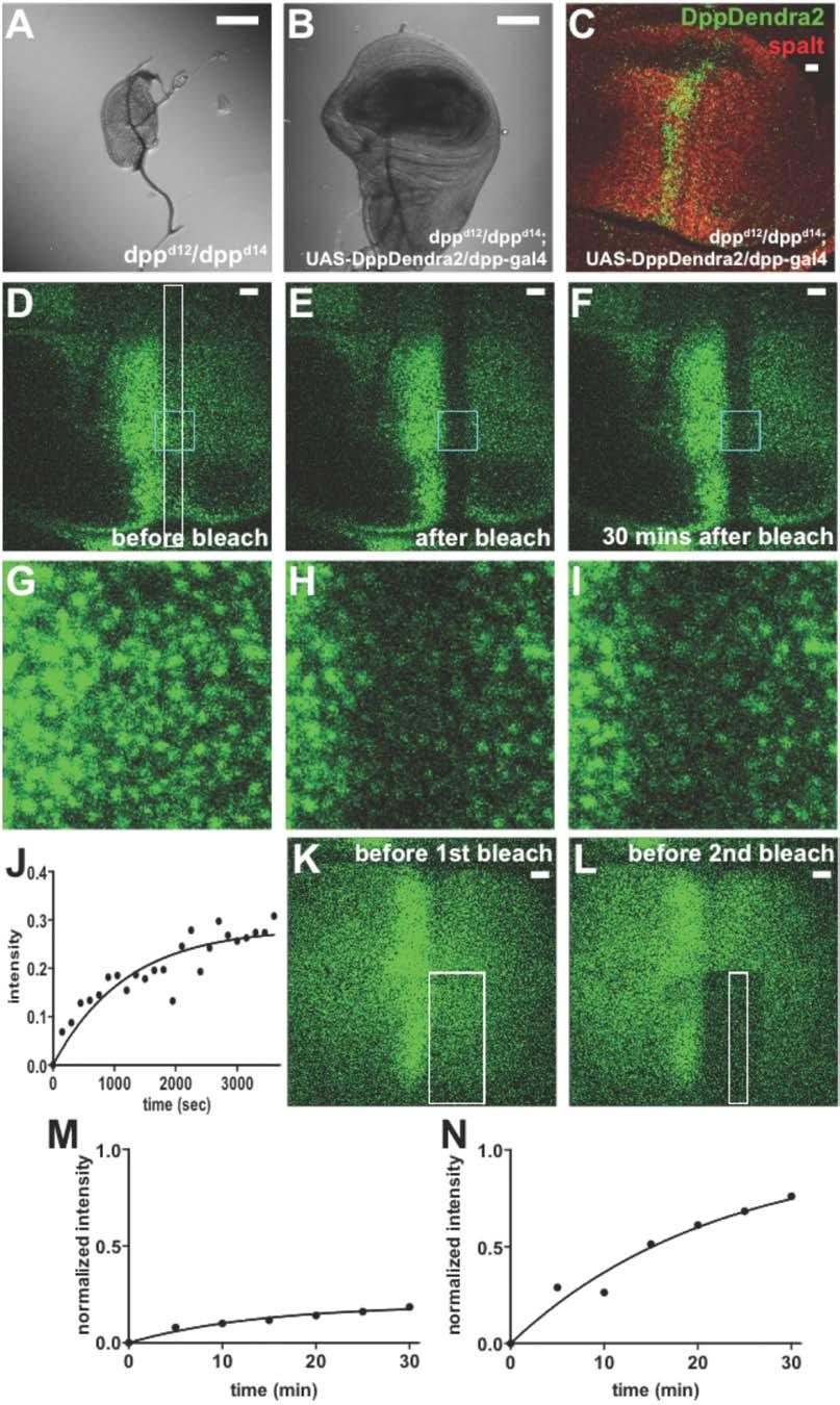
3 Figure S1. Fluorescence Recovery after Photobleaching of DppDendra2 (A-C) DppDendra2 is functional in vivo. Third instar wings discs from dpp d12 /dpp d14 (A) or dpp d12 /dpp d14 ; UAS-DppDendra2/dpp-gal4 (B) flies. Bar = 100 µm. Anti-spalt staining (C) of a wing disc from dpp d12 /dpp d14 ; UAS-DppDendra2/dpp-gal4 flies. Green: DppDendra2; red: antispalt. Bar = 10 µm. Comparisons of the sal staining patterns in such discs with those in wildtype discs revealed no significant difference in the location of the sal expression boundary (data not shown) (D-J) Time lapse imaging after photobleaching. A 150 µm x 10µm rectangular region (white box in D) adjacent to the Dpp source in a DppDendra2-expressing wing disc (genotype was UAS- DppDendra2/dpp-gal4) was photobleached. Thereafter five optical slices covering the apical 5 µm part of the disc were imaged every 2.5 minutes for 30 minutes. Slices from the same time point were maximum-projected to yield a single image, from which average fluorescence intensity was calculated. Bar =10 µm. (G-I) are magnified views of the region identified by a cyan box in D-F. (J) Fluorescence recovery was plotted as a function of time and fit to a single exponential function with a plateau of ~30% recovery (i.e. a 70% immobile fraction ). The halftime of recovery, based on this and two additional experiments, was 23.5 ± 7.7 minutes. (K-N) Use of pre-bleaching to suppress background due to an immobile (slowly-recovering) fraction. As shown in J, a substantial amount of bleached DppDendra2 in wing discs does not recover on a time scale of 1 hour (similar findings were observed by Kicheva et al., 2007, for DppGFP). When we bleached a 75 x 30 µm region of a wing disc DppDendra2 gradient (K), allowed it to recover for 30 minutes and then re-bleached a smaller region (75 x 10 µm) inside the first one (L), we observed that a much larger proportion of fluorescence recovered (M,N). This indicates that much of the immobile fraction can be suppressed by pre-bleaching. Since bleached molecules cannot be photoactivated, pre-bleaching potentially makes it posible to carry out photoactivation experiments in which a larger fraction of photoactivated molecules can be expected to be mobile (see Fig. S2).

4

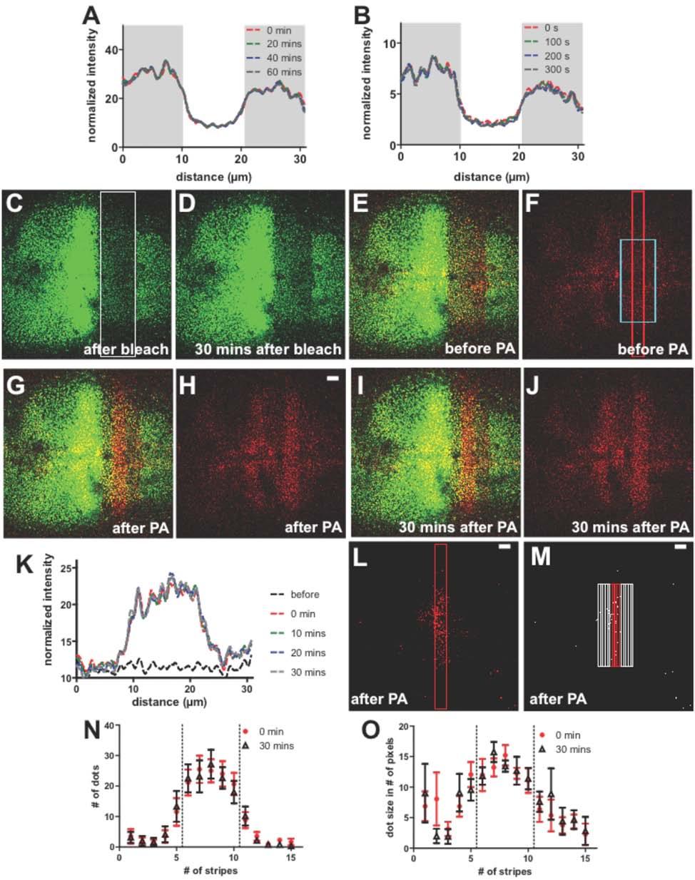
5 Figure S2. Lack of Fluorescence Spreading after DppDendra2 Photoactivation, Related to Figure 2 (A-B) Observations on short and long time scales. DppDendra2-expressing wing discs were photoactivated in two 10 µm-wide rectangular regions as in Figure 2, and followed using time lapse microscopy. Five optical slices covering the apical part of the disc were taken at each time point and maximum-projected into one image, from which intensity profiles were calculated. Graphs show intensity as a function of distance, with shaded gray areas corresponding to the photoactivated regions. In (A), time points were taken every 5 minutes for 1 hour; In (B), time points were taken every 5 seconds for 300 seconds. For illustration purpose, only the profiles at 20 minutes interval are shown in A, and only those at 100 seconds interval in B. (C-K) Lack of fluorescence spreading after photo-activation within a pre-bleached region. Prebleaching of a DppDendra2-expressing wing disc (UAS-DppDendra2/dpp-gal4) was performed as in Fig. S1K-N, except that a larger bleach area (white box in C; 150 x 30 µm) was used. After 30 minutes of fluorescence recovery (D-F), photoactivation (red box in F; 10 x 150 µm) was performed within the pre-bleached region (G-H), and followed for 30 additional minutes (I- J). In (K), intensity profiles along the horizontal axis of the cyan box in F were plotted at several time points. (L-N) Time lapse imaging of intracellular accumulations of DppDendra2 following photoactivation. Because pre-bleaching suppresses immobile background, by photoactivating DppDendra2 within a pre-bleached region, observations are confined to recently arrived molecules, which, in the transcytosis model, would be most likely to undergo further transport. In this experiment, we examined the numbers and size distributions of the punctate, intracellular accumulations of photoactivated DppDendra2 at the beginning and end of the experiment described in C-J. (L-M) Image processing. Gray-scale images (L) obtained as in C-J were subsequently converted into a binary images (M). The 10 µm wide photoactivated region, and two adjacent 10 µm-wide regions, were divided into a total of 15 2-µm wide stripes (i.e. stripes 6-10 refer to the photoactivated region; the Dpp source is to the left of stripe #1). Scale bar is 10 µm. (N-O) The distributions of the dots size and number of the dots immediately after photoactivation (red circles) and 30 minutes later (black triangles), are shown. Data were obtained from images using the Matlab command regionprops. Six independent experiments were used to calculate a mean and standard error of the mean (SEM). The dashed lines demarcate the two boundaries of the photoactivated ROI.

6 Figure S3. Measurement of Transport of DppDendra2 by FCS in Dally Mutant Wing Discs, Related to Figures 4A 4D Flies bearing a null mutation in dally (dally 80 ; kindly provided by Xinhua Lin [Han et al., 2004]), were crossed to generate the strain DppDendra2/ptc-gal4, gal80 ts ; dally 80 / dally 80. Ptc-gal4 was used instead of dpp-gal4 due to the location of dally and dpp-gal4 on the same chromosome. Gal80 ts was necessary to overcome the embryonic lethality of over-expressing Dpp under the ptc-gal4 driver. Briefly, embryos were kept at 18 C for the first 3 days and then shifted back to 25 C. FCS was performed essentially as in Figure 4, with minor differences in the hardware (Zeiss 710 instead of Zeiss 510 Meta+ConfoCor3), software (SimFCS, globally fitting data at multiple points, instead of ConfoCor3 software, fitting data at a single point). The data were well fit by a two-component model with slow and fast diffusion coefficients similar to those in Fig. 4. In wildtype discs, the two components contributed to the autocorrelation function in a 35:65 (slow:fast) ratio, very similar to that shown in Fig. 4. In dally mutant discs, this ratio showed a small change (to 48:52), that was not statistically significant. This suggests that the proportion of Dpp bound to cell surface dally is not large. Error bars in panel A represent SEM.

7 Figure S4. Pair Correlation Function Microscopy Demonstrates a Lack of Correlation between Extracellular and Intracellular DppDendra2, Related to Figures 4E 4G (A) Pair Correlation Function Microscopy was carried out in FM4-64-stained, DppDendra2- expressing wing discs, exactly as in Fig. 4, except that intensities were collected along a line perpendicular to a cell membrane (white dashed line in A; scale bar = 1 µm). The line was scanned with a pixel dwell time of 6.32 µs and a line time of 0.47 ms. (B) The intensity carpet. The horizontal and vertical axes represent positions along the line and time, respectively. Pixel colors represent fluorescence intensities, where warmer colors mean higher intensities. (C) Correlation carpets calculated from the intensity carpet. The autocorrelation functions (ACF) were calculated for all columns in the intensity carpet, and shown in the ACF total carpet. Columns (indicated by green arrow in A, and highlighted by the white box in C) are reiterated next to the pair correlation function at distance 8 (pcf8) for columns (indicated by yellow arrow in A). The horizontal and vertical axes represent position and time respectively. Pixel colors represent correlation strength, where warmer colors mean stronger correlations. (D) Average intensities of ACF carpet and pcf8 carpet from C. Notice the lack of positive correlation in pcf8 at any relevant time scale.

8 Figure S5. Controls for Time-Lapse Imaging (A) Photobleaching during image acquisition is minimal. Discs expressing cytosolic Dendra2 under the dpp-gal4 driver were imaged using identical settings as in FRAP assays. Fifteen z- stacks were acquired sequentially with no time delay between stacks. The mean intensities of stacks were plotted against the number of stacks. The intensity of the first stack was treated as one. Five replicates are shown. SEM is insignificant and thus neglected. (B) Imaging 8 nm Dendra2 solution with different laser power settings demonstrated that there was no dye saturation. Ten images were acquired at each laser power setting, from which the mean intensity was calculated. Intensity is in the unit of photons per pixel per pixel dwell time (two µs in this case). The data are well fit by a straight line. (C) Imaging 8 mm Dendra2 solution with different laser powers showed that there was no detector saturation under typical imaging settings. Detector saturation was observed at laser powers above 10%. Data obtained at powers up to 10% were well fit by a straight line. (D) Imaging various concentrations of Dendra2 solution under identical settings as in FRAP assays. The data show a linear relationship between fluorescence intensity and fluorophore concentration. Ten images were acquired for each concentration, from which the mean intensity was calculated. Intensity is in units of photons per pixel per pixel dwell time, and [Dendra2] is in nm. The data are fit by a line of slope=1, log 10 (intensity) = log 10 [Dendra2] (E) Step-wise photobleaching assay showing that fluorescence intensity is linearly related to fluorophore concentration in vivo. A DppDendra2-expressing wing disc was photobleached repetitively, and the mean intensity of the photobleached ROI was measured after each iteration. The mean intensity was then log transformed and plotted against the number of iterations. The data are well fit by a straight line.

9 Supplemental Experimental Procedures Table of Contents 1. Analysis: when can transport rates be inferred from FRAP kinetics? Background 1.1. A model of transport as a process in which a single species is being transported isotropically, and is subjected to constant degradation 1.2. A transport model in which transport is very fast, and transported molecules are rapidly taken up into an immobile compartment where they accumulate 1.3 The problem with transport by "restricted extracellular diffusion" 1.4 Summary 2. Simulation Background 2.1. Extracellular diffusion with uptake 2.2 Extracellular diffusion with uptake by saturable receptors; fitting "shibire-rescue" experiments 2.3 Simulation methods and results 2.4 Bicoid FRAP kinetics 3. "Spatial" FRAP Background 3.1. Analysis 3.2. Simulation 4. Estimating the concentration of free extracellular Dpp 5. Morphogen gradient dynamics and "non-receptors" Background 5.1. Extracellular diffusion with irreversible and reversible uptake in parallel 5.2. Non-receptors and co-receptors

10 1. Analysis: when can transport rates be inferred from FRAP kinetics? Background Whether recovery times observed in FRAP provide information about transport depends upon several time scales: (1) the time scale over which observations are being made, (2) the time scale over which transport occurs, and (3) the time scales of other processes that may affect the accumulation of molecules. Furthermore, when transport is by a random, isotropic process, such as diffusion, the characteristic time scale of transport depends upon the spatial scale of observation. In the sorts of studies in which FRAP is generally accepted as a valid means to measure parameters of transport, the spatial scale (size of the bleached region) and the time scale of observation are chosen so that other processes that affect the accumulation of molecules--such as synthesis, degradation, uptake into immobile compartments, etc., may be ignored. For example, when FRAP is used to study the diffusivity of integral membrane proteins, observation times tend to be on the order of seconds--fast relative to other processes in which membrane proteins may be involved. In the studies of Kicheva et al. (2007) on the transport of GFP-Dpp in the Drosophila wing disc, observation times were on the order of tens of minutes, in volumes with diameters on the order of 10 µm. Ultimately, Kicheva et al. inferred a rate constant for Dpp destruction on the order of 2.5 x 10-4 sec -1, which implies a destruction half-time of 46 minutes, similar to the time scale of observation. What is the impact on the interpretation of FRAP data when observation times are so close to morphogen half-lives? Here we explore this in the context of different transport models, focusing primarily on the Dpp gradient of the wing disc. In section 1.1, we show that, under conditions used by Kicheva et al., models of slow transport predict FRAP recovery curves that are very close in shape to simple exponential curves. In section 1.2, we show that models of fast extracellular transport with uptake into cells also predict FRAP recovery curves that are exponential in shape, provided that transported material accumulates in cells to a sufficiently high level. In section 1.3, we critique the recent, restricted extracellular diffusion model, which seeks to reconcile the slow transport rate reported by Kicheva et al., with data that cast doubt on planar transcytosis as a transport mechanism. Later, in section 2.4, we also extend some of this analysis to the Bicoid gradient of the Drosophila embryo A model of transport as a process in which a single species is transported isotropically, and is subjected to constant degradation. This could be taken to represent the model that Kicheva et al. consider for Dpp-GFP, in which the isotropic transport process is meant to be transcytosis, and degradation occurs during the time that molecules undergo transport. For simplicity, we consider here just a one-dimensional system--this will be a good approximation of the two-dimensional wing disc whenever the morphogen source and photobleached region are sufficiently large in one of the dimensions. This model can be written as (1) where D and k are constants. Assuming a discrete source and a semi-infinite domain, the steady state solution to (1) is

11 where λ = (D/k) 1/2, also known as the gradient length scale, and where c 0 is a function of the source boundary conditions. The length scale may be measured directly from the steady-state gradient shape, and in the case of the late third larval instar wing disc DppGFP gradient is approximately 20 µm. The time-dependent solution to (1) is (adapted from Bergmann et al, 2007) We simplify this by nondimensionalizing x to λ, and t to k, the time constant of degradation (i.e. define X= x/λ and τ = kt = Dt/λ 2 ) (2) (3) Consider a gradient that is at steady state at τ=0, where we completely photobleach a region from X=0 to X=, and then allow the gradient to recover due to the movement of molecules in from the source (at X<0). Then equation 3 will exactly describe the recovery of the gradient over time. Since we will make observations by averaging fluorescence intensity over some region of interest (e.g. a 10 µm-wide stripe), equation 3 is more useful in a form that averages from X=0 to some arbitrary point X=ξ. Integration gives us: This equation is even more useful if we normalize the result to the value within the region of interest prior to photobleaching (i.e. at its prior steady state): (4) The following plot shows the time evolution of this expression, for values of ξ = 0.25, 0.5, 0.75 and 1. Thus, these are the shapes of expected recovery curves, given a photobleaching experiment of the type described above. Accordingly, with such data, and knowing the width ξ of the region of observation, one could fit a value of τ. Dividing τ by the observation time would in turn yield k, and multiplying k by the square of the length scale λ would in turn give D. This is, in simplified form, the approach used by Kicheva et al. to infer a diffusion coefficient of 0.1 µm 2 sec -1 for DppGFP. In reality, the fitting procedure was more complicated, because the

12 above curves assume bleaching of the entire gradient, rather than just in the region of interest, but it is straightforward to extend the analysis allowing for recovery from both sides of a bleached interval, with results that are not too different, at least from the standpoint of the arguments that will shortly follow (since a much larger proportion of molecules recover from the source-side of a large bleached interval, than the non-source side). It is instructive to juxtapose the solution of (4) for ξ = 0.5 with the curve 1 Exp(-1.7τ). ξ=0.5 means a region of interest equal to 10 µm (assuming λ = 20 µm), a region of observation commonly used by Kicheva et al. 2007, and in the present study. This juxtaposition shows that the expected shape of the FRAP recovery curve, assuming this transport model (solid line), is only slightly different from the shape of a simple exponential recovery curve (dashed line). The difference in shape is well within the measurement uncertainties of a typical FRAP experiment, especially when one considers the large uncertainties that exist in initial values due to uncertain degrees of bleach-depth. The reason for pointing this out is that, as we shall see in the next section, other transport models--which do not involve transcytosis or slow transport--produce recovery curves with very similar shapes, but lead to estimations of diffusivity that can be extremely different A transport model in which transport is very fast, and transported molecules are rapidly taken up into an immobile compartment where they accumulate This is the sort of model one might have in mind for a morphogen that freely diffuses in the extracellular space, but then binds to cells, undergoes endocytosis, and eventually undergoes intracellular degradation. Such a model would minimally be described by a pair equations: To get a rough idea how this system behaves, we consider the limiting case in which transport is so fast that, after photobleaching a small region, transport is essentially complete before even the first observations are made. In that case, c 1 would return to near its pre-bleach value immediately. The solution for equation 2 would then be, where c 1 stands for the pre-bleach value of c 1. Since what we actually observe is the sum of c 1 and c 2, we add c 1 to the above expression to get (5) The limiting value of this expression as time goes to infinity is c 1 (1+k uptake /k deg ), which is therefore also the pre-bleach value of c tot. Thus we may express the above formula in terms of its pre-bleach value to get:

13 (6) Under the condition k deg <<k uptake, i.e. uptake being rapid compared with degradation, the coefficient in front of the exponential term is effectively unity. Then we get (7) What this tells us is that, for this simplified model, FRAP would produce a simple exponential recovery curve, reflecting only the time constant of degradation (because k deg <<k uptake ). In contrast, it is easy to show that, under the same circumstances, the steady-state gradient length scale associated with equation 5 will be approximately equal to (D/k uptake ) 1/2. To obtain equation 7 we made the approximation that diffusivity is so fast that c 1 achieves its steady state value immediately after photobleaching. How fast, in practice, does diffusion need to be in order for this approximation to be a good one? We note that the first equation in (5) is independent of the second and retains the same form as eq.1, with k uptake replacing k. Thus the steady state solution c 1 is simply c 1 (0,ss)Exp(x/λ), where c 1 (0,ss) is the steady state value of c 1 at x = 0, and where λ is understood as (D/k uptake ) 1/2. The second equation of (5) gives us the following relationship between the steady state values for c 1 and c 2. Defining c tot to mean c 1 +c 2, we find the steady state for c tot. where κ is defined as k uptake /k deg. Accordingly, the time dependent solution for c tot will be exactly the same as (2), provided that we now understand "k" in the definition of λ to mean k uptake. Thus, we may re-write the second equation in (5) as where c 1 (0,ss) stands for the value of c 1 at steady state at x=0, and where λ =(D/k uptake ) 1/2. Nondimensionalizing by making the substitutions X= x/λ and τ=k uptake t = Dt/λ 2, and substituting κ = k uptake /k deg, we get: (8) We also note that, because the steady state solution for c 1 is simply c 1 (0,ss)e -X, the second equation of (5) gives us the following relationship between the steady state values for c 1 and c 2 : c tot (X,ss) = (1+κ)c 1 (0,ss)e -X, where c tot (X,ss) is the sum of the steady state values for c 1 and c 2. If we define new scaled variables : χ 1 = c 1 /c tot (X,ss), and χ 2 = c 2 /c tot (X,ss), we may rewrite (8) as and the equation for χ 1 (from equation 3) as: (9) (10) We may then solve (9) numerically for χ 2, and add the result to the value of χ 1 obtained from equation 3 to yield the value of χ tot as a function of X and τ. Since X is defined relative to the

14 morphogen gradient length scale, which is 20 µm for the wing disc Dpp gradient, we shall examine the behavior of this system at a value of X = 0.25, which will be sufficient to give a sense of its behavior over the interval X={0, 0.5}. We shall plot a variety of values of κ (red=0.1; green =1, blue=5, black=20, orange=100) Recall that equation 7 gave us the approximate formula c tot (t)/c tot (0)= 1-Exp(-k deg t), which, if we convert to units of τ, becomes 1-Exp(-τ/κ), which we plot, using dashed lines, on top of the previous plot: c tot fraction of steady state time Comparing the two graphs, we see that the estimate c tot (t)/c tot (0)= 1-Exp(-k deg t) is an extremely good one for all κ>>1, i.e. whenever k uptake >> k deg. It is useful to point out that κ also corresponds to the ratio of c 2 to c 1 at steady state (this follows from the second equation in (5)). Thus, those cases in which a free extracellular diffusion model predicts that FRAP recovery should follow a simple exponential form which provides no information about parameters of transport are precisely those cases in which the internal pool of morphogen is much larger than the extracellular one. This is of course true of the wing disc Dpp gradient, in which at least 85% of Dpp is found intracellularly, i.e. c 2 /c 1 > 5.7 At the same time, it should be clear that, if one knows the actual value of of c 2 /c 1 at steady state, one could, in principle, infer a diffusion coefficient, because k deg can be determined from the FRAP recovery curve; given k deg, k uptake can be determined from c 2 /c 1, and given k uptake, D can be determine from the length scale λ = (D/k uptake ) 1/2. Specifically, if we let k stand for the observed FRAP rate constant, and ρ the observed ratio of c 2 /c 1, we get D eff = λ 2 ρk (11) Assuming λ = 20 µm and k (the time constant one obtains from an exponential fit of the FRAP data in Fig. S1), we get D eff 0.2ρ. Thus, ρ=10 would imply a diffusivity of 2 µm 2 sec - 1. ρ=100 would imply 20 µm 2 sec -1, and so on. In essence, the more Dpp that is found within, rather than between, cells, the faster diffusive transport should be.

15 A more intuitive way of putting this is, the faster the extracellular transport, the less Dpp needs to be involved in transport at any given time. With transport rates in the expected range for free extracellular diffusion (i.e. D between 10 and 100 µm 2 sec -1 ), we should expect ρ to be so high (70-666) that extracellular Dpp is between 0.15%-1.5% of total Dpp--all but unnoticeable by ordinary microscopy. In effect, a paucity of extracellular Dpp should not be interpreted as evidence against diffusive transport, but rather as evidence of in favor of it! Although these calculations are useful for illustrative purposes, the precise values one obtains do depend upon the details of the diffusive transport model in (5), which can be made more realistic by taking into account other compartments besides simply "extracellular" and "intracellular". For example, when we include an explicit cell-surface bound pool (equations 12), we see that the above constraints apply only to the "free" material, not that which is extracellular but bound to receptors. Accordingly, the value of ρ is not something we can, in practice, measure by ordinary imaging; we can only set a lower bound on it provided we are willing to neglect the effects of receptor saturation at high morphogen levels (to account for saturation, the rate constant could be replaced by a term that includes a dependency on morphogen level). In (12) we see at once that the first equation is unchanged from the first equation of (5), and the second and third equation, if summed, give an equation for c 2 +c 3 that is the same as the second equation in (5). Thus, the system evolves exactly like that in (5), except for the details of how the cell-associated morphogen is apportioned between the two pools. At steady state, the ratio c 1 :c 2 :c 3 will simply be 1:(k uptake /k deg ):(k uptake /k in ). Again, if c 1 (the extracellular free pool) is sufficiently small, the overall time constant for FRAP will reflect only k deg. In this case, however, only the extracellular free pool needs to be small. The extracellular bound pool (c 2 ) is not constrained. Therefore, to be compatible with diffusion coefficients on the order of µm 2 sec -1, it is not necessary that overall extracellular Dpp be 0.15%-1.5% of total Dpp, just that extracellular free Dpp be 0.15%-1.5% of total Dpp. Unfortunately, ordinary microscopic imaging techniques do not allow us to distinguish extracellular free and bound pools. One can extend (12) with any number of additional cell-associated compartments-in-series, without changing the above analysis. One case that is worth particular mention is the following, in which there are two separate internal pools c 3 and c 4, each degraded at a different rate. Such a model explicitly accounts for the so-called "immobile fraction" observed in FRAP, i.e. that there is a distinct proportion of photobleached material that does not recover on the time scale of observation. As long as observation times are very short compared with 1/k deg2 but not 1/k deg1, system 13, shown below, will behave just like (12), with the exception that fluorescence recovery will appear to plateau at a value less than what is observed prior to bleaching. (12)

16 1.3 The problem with transport by "restricted extracellular diffusion" In the "restricted extracellular diffusion" (RED) model proposed by Schwank et al., (2011), transport occurs by slow, undirected transfer among glypicans, rather than through free diffusion in the extracellular medium. There are two inherent difficulties with such a mechanism. The first is that it lacks a plausible biophysical basis. Glypicans are integral membrane proteins; our prima facie expectation should therefore be that interactions with glypicans should inhibit long range Dpp diffusion, not promote it (and studies with Xenopus BMPs strongly support this expectation [Ohkawara et al., 2002]). Presumably, what Schwank et al., are proposing is something along the lines of models that have been advocated in the proteoglycan literature, in which ligands transfer from one proteoglycan chain to another during the time they are bound. In this manner, ligands might diffuse along proteoglycans without the proteoglycans themselves having to move. Such models have always been hypothetical no direct or indirect evidence supporting such a mechanism has ever been found, and the most serious attempt to look for such evidence (Dowd et al., 1999, who looked at FGF diffusion through thick basement membranes) came out resoundingly against this idea. However, even if one posits that some kind of proteoglycan-facilitated transport can occur, there is a larger problem: binding of BMPs to glypicans (and heparan sulfate in general) is reversible, with modest affinity and relatively rapid kinetics. Thus, in the extracellular space there will necessarily be an equilibrium between glypican-bound Dpp and free Dpp, and there d be nothing to prevent the latter from diffusing. In order for the (hypothetical) transport of glypican-bound Dpp to be of any significance, it must carry a majority of the transport current (i.e. at least as many molecules per unit time must be traveling by this route as those traveling by free diffusion). This means that both that a very small fraction of Dpp molecules can be free (i.e. glypicans must be present at a sufficiently high level so that the equilibrium is shifted toward very few Dpp molecules being free), and that transport via glypicans must be sufficiently fast. Even to sustain an effective diffusivity of 0.1 µm 2 sec -1, the time constants associated with Dpp hopping off one proteoglycan and onto another would need to be so fast that it would seem unwise to simply assert that it can happen withough any direct evidence. The second problem with the RED model has to do with accounting for the distributions of Dpp within and around cells. Revisiting equation (5), and formula (11) which was derived from it, we see that, by the same token by which fast extracellular diffision requires that only a small fraction of the morphogen is in the transported pool, slow extracellular transport (i.e. RED) requires a rather large fraction of the morphogen to be in the transported pool (on the order of half, given the length scale of the gradient and the FRAP recovery kinetics). Schwank et al., are clearly aware of this, as they go to considerable efforts to argue that their clonal data support a model in which the vast majority (>80%) of Dpp is extracellular, albeit neither free nor receptorassociated. This conclusion disagrees with repeated, direct observations by many groups indicating that at least 85% of total fluorescence from Dpp-GFP (or, in the present study, Dpp- Dendra2) is found inside cells. The only potential explanation Schwank et al. give for ignoring (13)

17 such direct observations is their comment that the extracellular environment greatly reduces GFP fluorescence compared with the intracellular environment. This curious statement is made without any factual or experimental support, and it is difficult to imagine what experiments could have been done to support it (indeed, for Dendra2, which is ph-sensitive, it is more likely that intracellular fluorescence is somewhat suppressed, compared to extracellular). In contrast, their argument that most Dpp is extracellular is based on inferences that come from the staining of clones in Dpp-GFP-expressing discs. Their staining protocol is highly unusual, involving a one-hour incubation of live discs at room temperature, followed by brief washes and fixation. Unsupported assumptions are made that adequate staining of intracellular material will occur during such a short time period, that free Dpp will not be washed out during the washes, and that unbound antibody will not be trapped in the tissue. If, instead of dismissing the evidence that 85% of Dpp really is intracellular, we accept it, is there any way that the RED model could work? In principle, glypican-bound dally could cycle in and out of the cell, so that Dpp is still glypican-transported, but spends a great deal of time within cells. This, unfortunately, creates new problems. For example, there is just so fast that endoand exocytosis can occur, and the delays induced by it will necessarily retard transport. For example, a diffusion coefficient of 0.1 µm 2 sec -1 requires Dpp molecules to pass from one cell to the next within a fairly short interval of time (for a 1 µm-diameter cell, as in the wing disc, that interval would be 2.5 seconds). For the ratio of glypican-dpp inside the cell to exceed that on the cell surface by a factor "f", the internalization rate constant would need to exceed the externalization rate constant by the same factor. Putting this together implies that the internalization half-time would need to be 2.5/f seconds. In other words, to have 5 times the amount of glypican-dpp inside the cell as on the cell surface, one would need glypican-dpp complexes to be endocytosed with a half-life of 0.5 sec. In contrast, most measured internalization half-times (e.g. for growth factor receptors) are on the order of minutes or tens of minutes (Lauffenburger and Lindemann, 1993), and there is no evidence that proteoglycans can operate faster than this. Of course, the restricted extracellular diffusion model could be rescued by allowing intracellular glypican-dpp complexes to transfer directly from cell to cell without exocytosis back to the plasma membrane, but then such a mechanism would be formally equivalent to transcytosis, the implausibility of which is described elsewhere in this study. 1.4 Summary In summary, models of fast transport by free, extracellular diffusion with uptake into immobile pools, as well as models of slow transport, whether by transcytosis or "restricted" diffusion, are all fit by FRAP recovery curves that can have the approximate shape of the curve 1-e -kt. In the case of sufficiently fast diffusive transport, the time constant of this curve may have little or no relationship to parameters of diffusion (it can reflect only the time constant of degradation, a process that occurs after transport and uptake). The conditions that are required to produce this behavior are those in which uptake is sufficiently fast, compared with degradation, that a large amount of morphogen accumulates intracellularly. In contrast, in the case of slow transcytotic or "restricted" transport, this time constant will be related to diffusivity through the relationship k = λ 2 /D, allowing one to calculate D, given a known value of λ. Thus, in order to be able to infer a diffusion coefficient at all from FRAP experiments (such as those presented by Kicheva et al.), one must first assume a transport model other than free extracellular diffusion. Accordingly, the diffusion coefficient one obtains from fitting FRAP data to such a model can provide no evidence in support of the model itself--that would be circular reasoning.

18 2. Simulation Background In part 1, several assumptions were made to keep the analysis tractable. To show that the overall conclusions don't depend on these, we turn here to numerical simulation. We explore such simulations over a range of parameter values, and show that one can easily fit the FRAP data obtained both by Kicheva et al., and by ourselves. In section 2.1, we numerically explore a model in which there is free morphogen diffusion, binding of morphogen to receptors, internalization via those receptors, degradation of some of the internalized pool, and also transfer of some of the internalized pool to a very slowly-degrading compartment (the last condition being necessary, regardless of the model of transport, to explain the large, immobile fraction in FRAP). In section 2.2, we show how accounting for levels of receptor saturation consistent with predictions for the Dpp gradient (Lander et al., 2009) explains the shibirerescue experiments of Kicheva et al. (2007). In section 2.3 we present simulation code, and show how predictions were obtained for photoactivation experiments. In section 2.4 we discuss how some of the issues discussed here may explain some of the discrepancies in transport rate reported for Bicoid in the Drosophila embryo. It is important to point out that the primary purpose of data fitting in sections is not to "validate" any explicit, free diffusion-based transport model, i.e. to show that one or another of them is "correct", but rather to show that the data do not argue against these models, and therefore cannot be taken as providing any evidence against them (i.e. lending support for a transcytosis or "restricted diffusion" model). To this end, it is sufficient to be convinced that the models described are plausible (i.e. solely represent processes that are known to occur in vivo) and are analyzed over plausible regions of parameter space (i.e. realistic parameter values are used). We stress this point not because we lack confidence in any of the elements of the models we are proposing, but simply because we can never be certain of the completeness of such models--i.e. there may be other molecular processes going on of which we are not yet aware (e.g. other binding partners for Dpp), which could have additional effects on the spatial and temporal dynamics of gradient evolution. For explicit simulation, systems of equations were solved numerically using Mathematica software over appropriate spatial domains. Typically, we treated gradient formation as a onedimensional problem defined by an explicit production region, where Dpp is produced, adjacent to a receiving region, where Dpp is not produced. In some cases, equations were also explicitly solved in a two-dimensional domain to verify that the one-dimensional approximation was not significantly altering expected behaviors. In general, we used a production region size of 20 mm. Within the production region, equations for the rate of production of free Dpp were augmented with an additional, constant production term (since this term is the only parameter containing units of concentration, its value was set arbitrarily to 1, i.e. all concentrations may be understood as being expressed relative to it). Although more cumbersome, this approach is more appropriate for FRAP simulations than the simpler alternative of placing a constant-flux term at one boundary of a single gradient region (e.g. as done by Kicheva et al. 2007). This is because photobleaching--particularly when carried out close to the Dpp source--will rapidly lead to some depletion of Dpp within the source (due to transport into the bleached area), with the result that the flux across the source boundary cannot validly be treated as a constant. In the midpoint of the production region we placed a reflective boundary (zero-slope), reflecting the symmetry of the system (i.e. Dpp gradients from in both anterior and posterior directions). At the other end we placed an absorbing boundary, but always determined empirically that it was

19 far away enough from the production region that moving it still farther would have had no significant effect on the calculated results. Typically, absorbing boundaries were placed at 200 µm, and shown empirically not to have a significant effect on gradient profiles. In order to compare results from models with free extracellular diffusion to those that would be obtained under the assumption of transport by transcytosis, we modeled transcytosis in exactly the same way, either using a single equation for the "mobile fraction": i.e., ignoring the "immobile fraction", or by using two equations: (14) where the second equation explicitly accounts for the existence of a large "immobile fraction", i.e. a very slowly-recovering pool. To simulate FRAP and photoactivation experiments, values of Dpp-containing compartments at steady state were set to zero (or to some arbitrary fraction of their steady state values) within arbitrary spatial domains, and gradient recovery was followed over time. For example, to mimic the bleaching of a single 10 µm wide rectangular stripe (region of interest, or "ROI") immediately adjacent to the Dpp source--as shown in the image below--we commonly started with a steady state solution, and then set values of all variables to zero at time =0, between x=0 and x=10. (15) To simulate photoactivation in two 10 µm - wide stripes separated by 10 µm, we commonly set values of all variables to zero everywhere at time = 0, except between 0<x<10 and 20<x<30, where we used the steady state solution. 2.1 Extracellular Diffusion with Uptake Equations (13) were made more general by allowing for reversibility of uptake and movement into compartments, producing the following system:

20 (16) Equations (16) were numerically explored as described above under conditions corresponding to various FRAP experiments (see section 2.3). For example, the experiment of bleaching a 10 µm wide region of interest (ROI) next to the Dpp source was carried out by Kicheva et al., 2007 and produced sets of data shown in panel B below, along with curves fit according to a transcytosis model. One of these sets of data (green dots) was extracted and manually fit using equations (16), as shown below in panel C. A baseline value greater than zero was used in the plotting, in order to match the incomplete bleaching represented by the non-zero initial values in B. Clearly this is as good a fit to the data as those obtained by the transcytosis model. The parameters corresponding to the fit in panel C were D= 20 µm 2 sec -1 ; k on = 0.05 sec -1 ; k off = 5.4 x 10-7 sec -1 ; k in = 2.1 x 10-3 sec -1 ; k out = 5.3 x 10-5 sec -1 ; k t = 6 x 10-3 sec -1 ; k 1 =0.026 sec -1 ; and k 2 =7.6 x 10-5 sec -1. Numerical soluations were done as in Section 2.3. Note that, in this case, k off and k out are nearly zero, i.e. capture and internalization are effectively irreversible. Under these conditions, the gradient's length scale should be (D/k on ) 1/2 = 20µm, which agrees with observations. To determine how representative such parameter sets are of those that reasonably fit FRAP data, we explored 20,000 randomly-chosen parameter sets all of which, as a precondition, were required (1) to have a diffusion coefficient of 20 µm 2 sec -1 ; (2) to produce gradients with a length scale of approximately 20 µm and (3) to attain 50% of their long-time (100+ hour) values within 8 hours after initiation from initial conditions of zero in all compartments, and (4) to exhibit a lack of detectable spreading of total Dpp after photoactivation of stripes. The image below shows the distributions of parameter values in the 20 parameter sets that best fit the FRAP data. The ordinate scale is in units of log 10 of the rate constants (sec -1 ). The horizontal bars show the ranges of parameter values that were explored, and the vertical bars show values that were observed among the best-fit parameter sets. As expected, k 2 is necessarily slow in the best-fit parameter sets (to account for the observed "immobile fraction").

21 For these 20 parameter sets it is instructive to examine the fraction of Dpp at steady state that is in the free, extracellular pool; this is shown below. Horizontal bars indicate the values of the mean and standard deviation. Thus, as predicted, the best fit to the data occurs when the fraction of Dpp in the diffusible compartment is very small, often less than 1% of the total. 2.2 Extracellular diffusion with uptake by saturable receptors; fitting "shibire-rescue" experiments The rate constant k on in equations (16) is a pseudo-first order rate constant of binding, i.e. it models uptake as linear over all ranges of free Dpp concentration. It has been argued elsewhere (Lander et al., 2009) that Dpp receptors may be up to 50% saturated near the Dpp source, implying that the linear approximation of uptake is not strictly correct (see also section 4, below). Equations (16) can be modified to include receptor saturation by replacing k on with the true second-order rate constant k on multiplied by a concentration of free receptors that is equal to a constant (R tot, the total receptor concentration) minus the concentration of bound receptors, i.e. c 2. This approach is valid under the assumption that receptor trafficking and degradation dynamics are not themselves affected by Dpp (it is easy enough to introduce the necessary modifications to include such possibilities if they are). Thus equations (16) are replaced by Equations 17 were solved numerically for parameter sets and constraints similar to those used for equation 16. A value of R tot =2 was generally used, because it tended to ensure that receptor saturation (c 2 (x,t)/r tot ) would typically be 50% at x=0. (17)

22 Overall, the results obtained with equation 17 were not significantly different from those with equations 16. The most significant difference was noticed when attempting to fit the "Shibire rescue" data of Kicheva et al., In these experiments, photobleaching was carried out within a rectangular ROI in a disc in which endocytosis had been reversibly blocked. After a fixed period of time, a temperature downshift was used to restore endocytosis. Kicheva et al observed that fluorescence recovery was blocked during the period of inhibited endocytosis, and returned following the restoration of endocytosis. They inferred that endocytosis must be involved in the Dpp transport process. As we have seen above, however, viable models in which transport occurs by free extracellular diffusion are characterized by having a very large fraction of Dpp bound to, and inside of, cells. Since accumulation of Dpp inside cells cannot occur in the absence of endocytosis, such models will also exhibit a dramatic loss of fluorescence recovery under conditions of endocytic blockade, and this loss should be reversed when the endocytic blockade is removed. However, since the only source of Dpp degradation in such models is through Dpp uptake, they also predict that, under conditions of endocytic blockade, extracellular Dpp concentrations will continually increase to levels well above their pre-bleach values. With free Dpp levels that are normally very low (e.g. <1% of total), it is reasonable to think that such increases would not normally be detectable experimentally. However, under the model represented by equations 16, cell-surface bound Dpp should also rise during endocytic blockade. Since this pool may be large enough to detect experimentally, it is difficult to find parameter values that permit equations 16 to fit data such as those obtained by Kicheva et al., reproduced below (their Fig. S8, panel I), in which increases in total Dpp during the endocytic block period (white region, labeled "34 o C") are quite small. In contrast, under the model represented by equations 17, it is much easier to fit such data, because receptor saturation limits the amount by which cell-surface associated Dpp can increase. This is shown below: In this case, the parameter values were D= 20 µm 2 sec -1, k on = 0.05 sec -1, R tot = 2, k off = 2.7 x 10-6 sec -1, k in = 0.52 sec -1, k out = 4.7 x 10-4 sec -1, k t = 6.7 x 10-5 sec -1, k 1 =2.3 x 10-3 sec -1, k 2 =1.9 x 10-5

23 sec -1. As above, a non-zero initial condition was used to match the incomplete bleach depth in the experiment. 2.3 Simulation methods and results In this section we present the specific methods used for numerical simulations. We begin by making use of the general steady state solution for all models that, in the steady state, reduce to equation (1), over the domain 0<x<, with an explicit production region, from xmin<x<0 (where xmin is negative), in which free morphogen is produced at rate v. This solution can be found explicitly, and is: In the gradient "receiving" region, i.e. x>0, the average steady state value over an interval from x=x1 to x=x2 is just (18) where λ=(d/k) 1/2. To simulate a FRAP experiment we use these steady state values as initial conditions outside the photobleached region, and zero (or some arbitrary fraction of these initial conditions) within the photobleached region. Then we follow the evolution of the gradient back toward steady state. For example, in Figure 1 of the main text (reproduced below), the solid curve represents the solution to a transcytosis model, while the dashed curve represents the solutions to a model in which Dpp is transported only by free diffusion. To produce the solid curve, the following Mathematica code was used:

24 With systemt c 0,1 x, t Ifx 0, v, 0 d c 2,0 x, t k cx, t, cxmax, t 0, c 1,0 xmin, t 0, cx, 0 If0 x bleachboundary, 0, Ifxmin x 0, v k 1 xmin dk Cosh x xmin v, d k k 1 Cothxmin x d k dk, Withsettings xmin 10, xmax 200, tmax 3600, bleachboundary 10, params v 1, d 0.1, k , Blocksys systemt. Joinparams, settings, tm tmax. settings, xmn xmin. settings, xmx xmax. settings, b bleachboundary. settings, Λ d k. params, pdesol QuietFlattenNDSolvesys, c, t, 0, tm, x, xmn, xmx, PrecisionGoal 4, MaxStepFraction 1 100; plot1 ListPlotMap &, Λ 2 b Λ Λ v 1, 1b k 1Coth xmin. Joinparams, settings Λ MeanTablet, 0.32 cx, t. pdesol, x, 0.5, b 0.5, 0.5, t, 0, tm, 10, Joined True, PlotStyle Thick, PlotRange 0, Automatic, Frame True, FrameTicks 0, 1000, 2000, 3000, 0, 0.1, 0.2, 0.3, LabelStyle Medium Here, systemt represents equation (1) with the initial conditions as described in (18); settings fills in the distance to the midpoint of the production region (xmin), and the distance from x=0 to the bleach boundary (i.e. the width of the bleached region, which begins at x=0); and params fills in the parameters of transport and decay (D and k) corresponding to those inferred by Kicheva et al. pdesol gives a numerical solution, and plot1 calculates the average value of this solution over the bleached region, excluding 0.5 µ m at either edge, an normalizes it to the average value prior to bleaching. To produce the dashed curve, we begin with equations (16) for free extracellular diffusion with uptake, and solve for the steady state. Under these conditions, (16) reduces to a single ODE for c 1, and algebraic equations for c 2, c 3, and c 4. The equation for c 1 is simply (18), in which we take k to mean k on 1 k off 1 k out k 1 k t k in which we will refer to hereafter as k eff. It is useful to define c totss = c 1 +c 2 +c 3 +c 4, since this is the quantity corresponding to total fluorescence that would be measured in the microscope. It is thus straightforward to show that c totss = x Λ where λ=(d/k eff ) 1/2. The average value of c totss over an interval from x1 to x2 is therefore: x1 Λ v k 1 k 2 k in k off k on k in k on k t k 2 k in k on k t k off k on k out k t 1 Coth xmin k Λ 2 k in k on k 1 k t x2 Λ v Λ k 1 k 2 k in k off k on k in k on k t k 2 k in k on k t k off k on k out k t x1 x2 1 Coth xmin k Λ 2 k in k on k 1 k t Accordingly, the following Mathematica code was used to produce the dashed curve:,

25 WithsystemD c 0,1 1 x, t Ifx 0, v, 0 d c 2,0 1 x, t k on c 1x, t k off c 2x, t, c 2 0,1 x, t k on c 1x, t k off c 2x, t k in c 2x, t k out c 3x, t, c 3 0,1 x, t k in c 2x, t k out c 3x, t k t c 3x, t k 1 c 3x, t, c 4 0,1 x, t k t c 3x, t k 2 c 4x, t, c 1xmax, t 0, c 1,0 1 xmin, t 0, c 1x, 0 Α, k on k 1 k out k t c 2x, 0 k in k out k in k off k 1 k out k Α, t k in k on c 3x, 0 k in k out k in k off k 1 k out k Α, t k in k on k t c 4x, 0 Α. k 2 k in k out k in k off k 1 k out k t v Α If0 x bleachboundary, 0, Ifxmin x 0, keff 1 xmin dkeff Cosh x xmin, d keff v keff 1 Cothxmin x d keff dkeff. keff k on k off 1 k out k 1 1 k t k in Blocksettings xmin 10, xmax 200, tmax 3600, bleachboundary 10, params v 1, d 20, k on 0.05, k off , k in 0.52, k out , k t , k , k , Blocksys systemd. Joinparams, settings, tm tmax. settings, xmn xmin. settings, xmx xmax. settings,, b bleachboundary. settings, Λ d k in k on k 1 k t k 1 k in k off k in k t k off k out k t. params, pdesolb QuietFlattenNDSolvesys, c 1, c 2, c 3, c 4, t, 0, tm, x, xmn, xmx, PrecisionGoal 4, MaxStepFraction 1 100; plot2 ListPlot Map 1, 0.5 Λ b0.5 Λ v Λ k 1 k 2 k in k off k on k in k on k t k 2 k in k on k t k off k on k out k t 0.5 b Coth xmin k2 kin kon k1 kt. Joinparams, settings &, Λ MeanTablet, c 1x, t c 2x, t c 3x, t c 4x, t. pdesolb, x, 0.5, b 0.5, 0.5, t, 0, tm, 10, Joined True, PlotRange 0, 0.3, PlotStyle Red, Thick, Dashed, Frame True, FrameTicks 0, 1000, 2000, 3000, 0, 0.1, 0.2, 0.3, LabelStyle Medium Here systemd implements equations (16) according to the initial conditions described above, and pdesolb gives the numerical time-dependent solution. In order to simulate photoactivation, and the predicted subsequent accumulation of molecules in between two photoactivated stripes, we use a similar approach, but alter the initial conditions, and eliminate the production term (since, after photoactivation, it is assumed that no additional red-fluorescence is generated). For example, the following code uses systemtmod to represent these modified initial conditions for the transcytosis system, setting initial values to their steady-state levels in two stripes, from x=0 to x=10, and x=20 to x=30, with initial values being zero elsewhere. As before what is plotted is the average value over the region of interest (10.5<x<19.5). In this case, plotted values are normalized to the average value of the adjacent pixels in the photoactivated stripes (i.e. at x=10 and x=20) just after photoactivation

26 With systemtmod c 0,1 x, t d c 2,0 x, t k cx, t, cxmax, t 0, c 1,0 xmin, t 0, v cx, 0 If0 x boundary1, x dk, k 1 Cothxmin d k Ifboundary2 x boundary3, v k 1 Cothxmin x d k dk, 0, Blocksettings xmin 10, xmax 200, tmax 3600, boundary1 10, boundary2 20, boundary3 30, params v 1, d 0.1, k , Blocksys systemtmod. Joinparams, settings, tm tmax. settings, xmn xmin. settings, xmx xmax. settings, b1 boundary1. settings, b2 boundary2. settings, b3 boundary3. settings, Λ d k. params, pasol QuietFlattenNDSolvesys, c, t, 0, tm, x, xmn, xmx, PrecisionGoal 4, MaxStepFraction 1 100; plot3 ListPlot Mean Table v t, 0.32 cx, t Mean k 1 Cothxmin b1 dk v, d k k 1 Cothxmin b2 dk. d k Joinsettings, params. pasol, x, b1 0.5, b2 0.5, 0.5, t, 0, tm, 10, Joined True, PlotStyle Thick Likewise, for the system with free diffusion, we similarly modify initial conditions to obtain the following code: WithsystemDmod c 1 0,1 x, t d c 1 2,0 x, t k on c 1 x, t k off c 2 x, t, c 2 0,1 x, t k on c 1 x, t k off c 2 x, t k in c 2 x, t k out c 3 x, t, c 3 0,1 x, t k in c 2 x, t k out c 3 x, t k t c 3 x, t k 1 c 3 x, t, c 4 0,1 x, t k t c 3 x, t k 2 c 4 x, t, c 1 xmax, t 0, c 1,0 1 xmin, t 0, c 1 x, 0 Α, k on k 1 k out k t c 2 x, 0 k in k out k in k off k 1 k out k t Α, k in k on c 3 x, 0 k in k out k in k off k 1 k out k t Α, k in k on k t c 4 x, 0 Α. k 2 k in k out k in k off k 1 k out k t Α If0 x boundary1, v keff 1 Cothxmin x dkeff, d keff v Ifboundary2 x boundary3, keff 1 Cothxmin x d keff dkeff, 0. keff k on k off 1 k out k 1 1 k t k in, Blocksettings xmin 10, xmax 200, tmax 3600, boundary1 10, boundary2 20, boundary3 30, params v 1, d 20, k on 0.05, k off , k in 0.52, k out , k t , k , k , Blocksys systemdmod. Joinparams, settings, tm tmax. settings, xmn xmin. settings, xmx xmax. settings, b1 boundary1. settings, b2 boundary2. settings, b3 boundary3. settings, Λ d k in k on k 1 k t k 1 k in k off k in k t k off k out k t. params, pasolb QuietFlattenNDSolvesys, c 1, c 2, c 3, c 4, t, 0, tm, x, xmn, xmx, PrecisionGoal 4, MaxStepFraction 1 100; plot4 ListPlot MeanTablet, c 1 x, t c 2 x, t c 3 x, t c 4 x, t Meanc totss. x b1, c totss. x b2. Joinsettings, params. pasolb, x, b1 0.5, b2 0.5, 0.5, t, 0, tm, 10, Joined True, PlotRange All, PlotStyle Green, Thick Below, we show the results of both simulations on the same graph (transyctosis model in blue; free diffusion model in red, dashed), along with experimental data points (black triangles) taken from Figure 2.

27 relative fluorescence Note the values on the ordinate. The transcytosis model predicts that Dpp fluorescence should rise to a level of about 15% of the initial level in adjacent photoactivated stripes, whereas the free diffusion model predicts an increase in fluorescence between photoactivated of less than 0.5 %, a much better fit to the data. What about the "restricted extracellular diffusion" model? As stated in section 1.3, the equations for this model can be treated as identical to those for free extracellular diffusion, with c 1 representing extracellular glypican-bound Dpp. By virtue of this, the reactions represented by k on and k off must be taken to mean the rate constants for transfer from being glypican-bound to being receptor-bound. Assuming we give k off its usual value (negligiably small), we find that k on is fixed by the length scale of the gradient, because that length scale must equal (D/k on ) 1/2. Setting D=0.1 µ m 2 sec -1, making these modifications, and re-running the simulation used to generate the dashed, red curve in the above plot, we obtain relative fluorescence time time Clearly, as with transcytosis, slow transport correlates with the expectation that a substantial fraction of photoactivated Dpp should spread. We may also look at the response to photoactivation spatially. Here the different curves represent fluorescence profiles for the free diffusion model at times equal to 0, 200, 400 and 1000 seconds after photoactivating stripes from 0<x<10 and 20<x<30. fluorescence distance To mimic photoactivation following pre-bleacing and 30 minutes of recovery (Fig. S2), we first obtain a solution for the bleaching and then use it as initial conditions for the photoactivation. Here we show results for the transcytosis model (blue) and the free diffusion model (red, dashed), using the same parameters as above, and plot these together with experimental data from Figure S2):

28 relative fluorescence time Clearly, the data fit the extracellular diffusion model much better than they fit the transcytosis model. 2.4 Bicoid FRAP kinetics Gregor et al., (2007) used FRAP to estimate the rate of Bicoid transport within Drosophila embryos, obtaining a value of 0.27 µm 2 sec -1. The data, shown below, were obtained using 2- photon bleaching near the anterior-most point of the embryo. The bleached volume was described as having dimensions 16 x 16 x 7 µm. The above fit to the data was obtained, according to the authors, using the formula of Brown et al. (1999); this is a rather general formula with many terms, but the gist of it is easily appreciated: The mean time t, in three dimensions, required for free diffusion to carry a particle with diffusion coefficient D, over a distance x, is simply x 2 /(6D). In the above experiment, the shortest path along which molecules must travel in order to reach the center of the bleached volume (16 x 16 x 7 µm) is simply half the shortest dimension of that volume, i.e. 7/2 = 3.5 µm. Plugging this in gives t=3.5 2 /(6D) 2/D. Thus D 2/t. As the half-time to recovery after photobleaching, read off the above figure, is about 8 seconds, this yields an estimate of D = 2/8 = 0.25 µ m 2 sec -1, quite close to the value obtained by fitting the more general equation. Recently, Castle et al., (2011) pointed out that the fact that photobleaching is not instantaneous, but rather requires several seconds, necessitates an upward correction of about 3-fold to this estimate. As in the studies of Kicheva et al., 2007, the validity of the FRAP approach for estimating a diffusion coefficient depends upon the assumption that other processes that affect the accumulation of fluorescence are not occuring on the time scale of observation. As in the case of Dpp in the wing disc, it is obvious that the above data could just as easily be fit by a simple exponential recovery curve, raising the possibility that the recovery being observed is not recovery due to slow diffusion, but recovery due to slow accumulation after fast diffusion (i.e.

29 diffusion that is essentially complete by the time the first observations are made). The recent measurements made by Abu-Arish (2010) suggest that Bicoid's true diffusivity is actually about 7 µ m 2 sec -1. At that rate, the mean time to traverse 3.5 µm should be only 0.3 seconds. Significantly, Gregor et al., point out that the duration of the pulse required to produce photobleaching in their experiments was itself 5 seconds long, so any molecules moving with a diffusivity of 7 µm 2 sec -1 should have essentially equilibrated across the bleached volume by the time of the very first observations. What then could account for the recovery, with a half-time of 8 seconds, that Gregor et al., observed? In the case of DppGFP in the wing disc, we eventually concluded that the time constant of recovery observed by Kicheva et al. largely reflected the time constant of Dpp degradation. In the Bicoid case, however, this is unlikely to be so, because the rate of Bicoid degradation has recently been measured (Drocco 2011, Ph.D. thesis), and is much too slow (t 1/ minutes). A more likely explanation is that Bicoid simply binds, reversibly, to sites that are effectively immobile (during the observation time), and accumulates as a result. Under such circumstances, the time constant of accumulation would reflect the time constant of dissociation from those immobile sites. Consider the following scenario: Bicoid normally diffuses freely, but binds with (pseudo) first order rate constant k on to some immobile or very slow moving sites in the cytoplasm (e.g. cytoskeleton), and dissociates from those sites with rate constant k off. Assuming binding sites are in excess, the total fraction of Bicoid that will be bound to such sites, at equilibrium, will simply be 1/(1+ k off /k on ). As long as k on is more than a few fold faster than k off, most of the Bicoid will be bound. However the rate constant associated with accumulation of Bicoid will be k off. Thus, if we choose k off =ln2/8 = sec -1, and k on several fold higher than this (e.g sec -1 ), we'd expect that ~25% of total Bicoid would recover within the first second (and therefore not be detected in the experiment), while 75% would recover following the curve 1-e t, shown below in green, which reasonably fits the observed data. We note that this behavior, in which FRAP systematically underestimates the diffusivity of a molecule due to reversible binding during the time of observation has been analyzed by others (Sprague et al, 2004). One of the simplest ways to demonstrate that recovery such as that shown above is due to binding and not transport is to show that the time constant of recovery does not scale with the size of the bleached spot (within limits). According to recent work (Drocco 2011, Ph.D. thesis) this is apparently the case for Bicoid, strongly suggesting that the above explanation is correct. This approach is conceptually similar to that described as "spatial FRAP" in the main body of the text, and discussed in the next section.

30 3. Spatial FRAP Background In section 1, we argued that FRAP cannot generally be used as a means to measure transport rates if accumulation or destruction processes occuring downstream of transport are significant on the timescale of observation. This argument is predicated on the notion that FRAP is being performed at a single location, i.e. data are averaged over a single region of interest (ROI) In principle, if one bleaches a large ROI, and measures recovery at more than one location within that ROI, then a comparison of the differences in recovery times at different locations should, in principle, enable one to "subtract out" the contributions to recovery that come from processes downstream of transport, and extract transport parameters themselves. Aware that such "spatial FRAP" might provide useful insights into transport parameters, Kicheva et al. (2007) performed a small number of experiments of this type, which are reported in their supplemental online material. Although they fit the results to a model of transcytotic transport, they did not explicitly address whether other models might fit the data equally well. Here we address this issue. In section 3.1, we mathematically analyze the general predictions of spatial FRAP experiments, and re-analyze the spatial FRAP data of Kicheva et al. (2007). In section 3.2, we present the code used for the simulations of spatial FRAP, according to different transport models, that is provided in Figure 3C-D of the main text. 3.1 Analysis As shown by equation 3, according to the transcytosis model, the rate of recovery after photobleaching displays an explicit dependence on location (i.e., X in equation 3). It is useful to express this dependence in terms of the rate of approach to steady state as a function of distance from the boundary between a photobleached and non-photobleached region. We may define the rate of approach to steady state in terms of the time τ at which the value of c at any location X has returned to 1-1/e of its pre-bleach (i.e. steady state) level. Explicitly solving equation 3 for τ as a function of X is not possible, but we may solve it numerically, and plot the result. Here we examine, on the abcissa, values of X from 0 to 1. Recalling that X = x/λ, this means, for the Dpp gradient, values of x from 0 to 20 µm. Although this result is not truly a straight line, it is very close to one, and can be fit by the function τ 0.59X From this we can ask, how much of a change in X would be required to produce a given change Δτ in the rate of recovery after photobleaching. Δτ = (0.59X ) - (0.59 X ) = 0.59 ΔX Recalling that τ = kt, we get that Δt =0.59ΔX/k. Using the value of k = 2.5 x 10-4 from Kicheva et al., we obtain Δt =2360ΔX. Thus a positional shift of 10 µm (ΔX=0.5) should produce a delay in

31 recovery of about 1200 seconds. In contrast, for a system of transport by free extracellular diffusion, coupled to rapid uptake and degradation, we know from the analysis in section 1.2, that for large κ (uptake that is fast relative to degradation), the spatial dynamics of the entire system will be governed by an equation identical to equation 3, except in so far as the definition of λ is understood as corresponding to (D/k uptake ) 1/2, rather than (D/k deg ) 1/2. Using the value of k uptake =0.05 that results from setting the diffusion coefficient to 20 µm 2 sec -1 and the length scale to 20 µm, we obtain Δt = 12ΔX. Thus, a positional shift of 10 µ m should produce a delay in recovery of about 6 seconds. Similarly, we may estimate the expected delay in recovery for a "restricted extracellular diffusion" model by using a much lower value of D in the above calculation. For example, for D=0.1, we need set k uptake =2.5 x 10-4, which in turn gets us right back to Δt =2360 ΔX, just as in the transcytosis model. Thus, in summary, slow transport predicts a long delay in recovery (regardless of which model is used); fast transport predicts a short one. In principle, one should be able to detect a difference in delay between 6 and 1200 seconds experimentally. The ideal circumstances for doing this would involve photobleaching a very large ROI (ideally the entire gradient), and observing recovery in rectangles spaced at various distances from the source in the same disc (e.g µm, µ m, µm, etc.). As it happens, none of the experiments reported by Kicheva et al. (their figure S4) correspond to this configuration. In one case, results with a single 20 µm wide rectangle in one set of discs was used and compared with a 10 µm wide rectangle in a different set of discs. In another, a series of nonoverlapping 10x10 µm boxes were compared. In a third case, a 30x30 µm ROI was bleached, and fluorescence recovery in the entire box was compared with that in a 10x10 µm box in the center of the ROI. In the first case it is difficult to determine whether there is any delay in recovery as a function of distance, especially when taking into account the substantial differences in "immobile fractions" that resulted from comparing different discs. In the second case it is difficult to determine whether there is any delay in recovery because, after about the second box, all signals are so close to background that they can be fit by a curve of almost any shape. Moreover, in this configuration, the significant diffusion of Dpp from regions dorsal and ventral to each box would be expected to dramatically decrease the expected delay at each location (i.e. much of the advantage of spatial FRAP in distinguishing among transport models is lost in this scenario). The third case comes closest to the ideal configuration. In this case, Kicheva et al., fit the data with curves that suggest a delay of about 250 seconds between the central box and the entire box (see panels below, reproduced from Kicheva et al., 2007, Figure S4). Because the data for the entire box (black data points) averages the recovery at a variety of distances (from 0 to 30 µm), not just the first 10 µm, a delay of 250 seconds between the black and red curves is indeed consistent with the transcytosis model (see section 3.2).

32 On close examination of the data, however, we noticed that the red curve-fit is not particularly good, and depends heavily on the very first data point. There are several potential problems with both the data and the analysis in this figure. For example, the red data points appear to assymptotically approach a value about 20% below the black points. Given the exponential shape of the gradient and its length scale, the steady state value within the red box should be 92% of the average steady state value in the white box, so the red data points should assymptotically approach a value only 8% below the black ones. This discrepancy suggests that there is some systematic error in the data collection The simplest way to correct for this is to normalize both the red and the black data points to their (apparent) steady state values. This was done in the curve below. From this perspective it is clear that the overall dynamics of recovery within the red box differs only slightly from that in the black box, with the major difference occuring within the first few hundred seconds, and even then being quite small (much smaller than the 250 second delay predicted by slow transport models). Intensity Time sec Although we cannot know the reason why the small-box data did not asymptotically approach the correct value in these experiments, a reasonable possibility is that the larger, white box was placed too close to the Dpp production region, and therefore overlapped territory in which GFP- Dpp is produced (the figure presented along with the data suggests that this may well have been the case). We were careful to avoid such overlap in the experiments shown in Figure 3 of the main article. 3.2 Simulation This section presents the methods used to simulate the expected results of spatial FRAP, as presented in Figure 3 of the main text First, we consider the model of transcytotic transport, in which there is a single mobile species, and values of D and k correspond to those inferred by Kicheva et al. (referred to as systemt in section 2.3, and with the same parameters as used there). As before, we set the midpoint of