Pointwise Shape-Adaptive DCT Image Filtering and Signal-Dependent Noise Estimation

Transcription

1 Julkaisu 710 Publication 710 Alessandro Foi Pointwise Shape-Adaptive DCT Image Filtering and Signal-Dependent Noise Estimation Tampere 2007

2 Tampereen teknillinen yliopisto. Julkaisu 710 Tampere University of Technology. Publication 710 Alessandro Foi Pointwise Shape-Adaptive DCT Image Filtering and Signal-Dependent Noise Estimation Thesis for the degree of Doctor of Technology to be presented with due permission for public examination and criticism in Tietotalo Building, Auditorium TB111, at Tampere University of Technology, on the 5th of December 2007, at 12 noon. Tampereen teknillinen yliopisto - Tampere University of Technology Tampere 2007

3 ISBN (printed) ISBN (PDF) ISSN

4 Abstract When an image is acquired by a digital imaging sensor, it is always degraded by some noise. This leads to two basic questions: What are the main characteristics of this noise? How to remove it? These questions in turn correspond to two key problems in signal processing: noise estimation and noise removal (so-called denoising). This thesis addresses both abovementioned problems and provides a number of original and effective contributions for their solution. The Þrst part of the thesis introduces a novel image denoising algorithm based on the low-complexity Shape-Adaptive Discrete Cosine Transform (SA-DCT). By using spatially adaptive supports for the transform, the quality of the Þltered image is high, with clean edges and without disturbing artifacts. We further present extensions of this approach to image deblurring, deringing and deblocking, as well as to color image Þltering. For all these applications, the proposed SA-DCT approach demonstrates a state-of-the-art Þltering performance, which is achieved at a very competitive computational cost. The second part of the thesis addresses the problem of noise estimation. In particular, we consider noise estimation for raw-data, i.e. the unprocessed digital output of the imaging sensor. We introduce a method for nonparametric estimation of the standard-deviation curve which can be used with non-uniform targets under non-uniform illumination. Thus, we overcome key limitations of the existing approaches and standards, which typically assume the use of specially calibrated uniform targets. Further, we propose a noise model for the raw-data. The model is composed of a Poissonian part, for the photon sensing, and a Gaussian part, for the remaining stationary disturbances in the output data. The model explicitly takes into account the clipping of the data, faithfully reproducing the nonlinear response of the sensor when parts of the image are overor under-exposed. This model allows for the parametric estimation of the noise characteristics from a single image. For this purpose, a fully automatic algorithm is presented. Numerous experiments with synthetic as well as with real data are presented throughout the thesis, proving the efficiency of the proposed solutions. Finally, illustrative examples, which show how the methods proposed in the Þrst and in the second part can be integrated within a single procedure, conclude the thesis. iii

5 iv Abstract

6 Foreword This thesis is based on part of the research work which has been carried out by the author between May 2005 and August 2007, at the Institute of Signal Processing of Tampere University of Technology (TUT), Finland. Effectively, this work can be seen as a direct continuation and further development of the methods and results presented in the author s earlier doctoral thesis in Mathematics [47], defended in May 2005 at the Department of Mathematics of Politecnico di Milano, Italy. This work has been accomplished under the supervision of Professors Karen Egiazarian and Vladimir Katkovnik. I am greatly indebted towards both of them, for their highly professional guidance and for being incessantly patient and supportive. The high trust they have placed in me is possibly the greatest reward of my endeavors. My special thanks go to Professors Jaakko Astola, director of the Signal Processing Algorithm Group (SPAG) and of Tampere International Center for Signal Processing (TICSP), and to Moncef Gabbouj, director of the Institute of Signal Processing, for the excellent research environment which they have offered me since I came to Tampere in November The work presented in this thesis has been done within research projects of the Academy of Finland s Finnish Centre of Excellence program, of Nokia Research Center (NRC), Tampere, and of Tekes, the Finnish Funding Agency for Technology and Innovation. Without their Þnancial support, gratefully acknowledged, this research would have not been possible. This thesis is dedicated to the fragile and inspiring beauty of the Finnish Nature and especially to lake Särkijärvi, where many of the ideas enclosed in this volume took shape. Tampere, November 2007 Alessandro Foi v

7 vi Foreword

8 Contents Abstract Foreword Contents iii v vii Introduction to the thesis xi Outlineofthethesis... xi Publications... xii Notationandconventions... xiv I Pointwise Shape-Adaptive DCT Þlters 1 1 Pointwise Shape-Adaptive DCT denoising and deblocking Introduction Observationmodelandnotation AnisotropicLPA-ICI Shape-AdaptiveDCTtransform OrthonormalShape-AdaptiveDCT Meansubtraction Coefficientalignment Non-separability and column-row (CR) vs. row-column (RC) processing PointwiseSA-DCTdenoising Fast implementation of the anisotropic neighborhood Localestimates Global estimate as aggregation of local estimates Wiener ÞlteringinSA-DCTdomain Pointwise SA-DCT for deblocking and deringing of block-dct compressedimages Motivation Modeling Pointwise SA-DCT Þltering of color images with structural constraintinluminance-chrominancespace Luminance-chrominancespace vii

9 viii Contents Pointwise SA-DCT denoising in luminance-chrominance space Deblocking and deringing of B-DCT compressed color images Experimentsandresults Grayscaledenoising Colordenoising Deblockingandderinging Subjectiveperceptualquality Complexity Discussion Conclusionstothechapter Pointwise SA-DCT regularized deconvolution Regularizedinverse Adaptiveanisotropictransformsupport PointwiseSA-DCTdeblurring Thresholding with adaptive variance in transform domain Adaptiveweightsandglobalestimate RegularizedWienerinverse Fast computation of coefficients variance Experiments Somecommentsontheapproach Synthesis with ψ (i)ª i Analysis with ψ ù (i)ªi Ill-posednessandregularization Intermediatecases;comments;vaguelettes Practicalaspects Decouplingofthetransformandtheinversion Global Fourier-domain inverse, periodicity, and localized processing Extensions Signal-dependent noise removal Introduction Signal-dependentnoisemodel Algorithm Stage 1: Hard-thresholding in Pointwise SA-DCT domain Stage 2: Wiener Þltering in Pointwise SA-DCT domain Complexity Experimentalresults Deblurring of images corrupted by signal-dependent noise Shape-adapted bases by orthonormalization Constructionofa shape-adapted basis ModiÞcationstothealgorithms Experiments Denoisingexperiments Deblurringexperiments... 81

10 ix Appendix A: LPA-ICI 85 A.1 LocalPolynomialApproximation(LPA) A.2 Intersection of ConÞdenceIntervals(ICI)rule Appendix B: A gallery of basis elements 89 B.1 Supports B.2 Arrangement of the Þgures B.3 Interestingsightsinthegallery B.4 Thegallery II Signal-dependent noise measurement, modeling, and Þtting for digital imaging sensors 117 Preface Noise measurement for raw-data by automatic segmentation of non-uniform targets Introduction Observationmodel Themethod Acquisitionandaveraging Segmentation Measurementofthestandarddeviation Experimentalresults Setup Segmentation Standard-deviationcurves Aparametricmodel Conclusionstothechapter Practical Poissonian-Gaussian noise modeling and Þtting for single image raw-data Poissonian-Gaussianmodeling Raw-datamodeling Heteroskedasticnormalapproximation Thealgorithm Waveletdomainanalysis Segmentation Local estimation of expectation/standard-deviation pairs Maximum-likelihood Þtting of a global parametric model Clipping(censoring) Clippedobservationsmodel Expectations, standard deviations, and their transformations Expectation and standard deviation in the wavelet domain Algorithm:clippedcase Local estimation of expectation/standard-deviation pairs Maximum-likelihood Þttingoftheclippedmodel Robustestimates

11 x Contents Robuststandard-deviationestimates Maximum-likelihood Þtting(non-clipped) Clippedobservations Anotherexample Experimentswithrawdata Comments Different parametric models for the σ function Multipleimages Denoisingclippedsignals Interpolation of the functions S m, S e, S r, E r AlternativestotheMADestimator Alternativestoleast-squaresinitialization Conclusionstothechapter Conclusions to the thesis 173 C.1 Overview C.2 Futureresearch C.3 Automaticnoiseanalysisandremovalforraw-data Bibliography 181

12 Introduction to the thesis Outline of the thesis The thesis is structured in two self-contained parts. The Þrst part deals with a family of image Þltering algorithms collectively called Pointwise Shape-Adaptive DCT Þlters. The key idea of these algorithms is to use a shape-adaptive transform on a support that adapts to the images features. SpeciÞcally, we use the low-complexity SA-DCT transform [154] in conjunction with the Anisotropic Local Polynomial Approximation (LPA) - Intersection of ConÞdence Intervals (ICI) technique [47],[91],[92], which deþnes the shape of the transform s support in a pointwise adaptive manner. The thresholded or attenuated SA-DCT coefficients are used to reconstruct a local estimate of the signal within the adaptive-shape support. Since supports corresponding to different points are in general overlapping, the local estimates are averaged together using adaptive weights that depend on the region s statistics. Besides a basic grayscale image denoising Þlter for additive white Gaussian noise (Chapter 1, Section 1.5, p. 11), we present extensions of the approach to: - color image Þltering (Section 1.7, p. 24); - deringing and deblocking of B-DCT compressed image (e.g., JPEG images) (Section 1.6, p. 20); - deconvolution (deblurring) (Chapter 2, p. 49); - signal-dependent noise removal (Chapter 3, p. 65). A separate chapter is dedicated to another class of transforms deþned on arbitrarily shaped supports, the so-called shape-adapted bases (Chapter 4, p. 77). In particular, we evaluate their Þltering performance when they are used within the above algorithms in place of the more efficient SA-DCT. An appendix on the LPA-ICI technique is provided for the reader s convenience (Appendix A, p. 85). Several illustrations of the different basis elements used in the considered shape-adaptive and shape-adapted transforms are given at the end of this Þrst part (Appendix B, p. 89). The second part of the thesis deals with noise estimation for the raw-data of digital imaging sensors. This part comprises two chapters. First (Chapter 5, p. 123), we present a nonparametric method for estimation of the curve which describes the standard-deviation of the noise as a function of the expectation of the xi

13 xii Introduction to the thesis pixel raw-data output (so-called standard-deviation function ). This method relies on the analysis of several images captured under the same Þxed acquisition and illumination conditions. However, we do not require the target or the illumination tobeuniform. Basedonanautomaticsegmentation of the images, we separate samples with different expected output and estimate their standard-deviations. Thus, while other techniques require a uniform target (e.g., a test-chart), in our approach we beneþt from the target non-uniformity by simultaneously estimating the standard-deviation function over a large range of output values. The most signiþcant contributions of this second part are given in the subsequent chapter (Chapter 6, p. 135), where we propose a noise model for the raw-data and an algorithm for the fully automatic estimation of these parameters from a single noisy image. The model is composed of a Poissonian part, for the photon sensing, and Gaussian part, for the remaining stationary disturbances in the output data. The model explicitly takes into account the clipping of the data, faithfully reproducing the nonlinear response of the sensor when parts of the image are over- or underexposed. The parameter estimation algorithm utilizes a special maximum-likelihood Þtting of the parametric model on a collection of local wavelet-domain estimates of mean and standard-deviation. Experiments with synthetic images and real raw-data from camera sensors demonstrate the effectiveness and accuracy of the algorithm in estimating the model parameters and conþrm the validity of the proposed model. Conclusive remarks and few illustrative examples, which show how the methods proposed in the Þrst and in the second part can be integrated within a single procedure, are given at the end of thesis (Conclusions, p. 173). Publications and author s contribution Most of the material presented in this thesis appears in the following publications by the author: [58]: Foi, A., V. Katkovnik, and K. Egiazarian, Pointwise Shape-Adaptive DCT for High-Quality Denoising and Deblocking of Grayscale and Color Images, IEEE Trans. Image Process., vol. 16, no. 5, pp , May [59]: Foi, A., V. Katkovnik, and K. Egiazarian, Pointwise Shape-Adaptive DCT denoising with structure preservation in luminance-chrominance space, Proc. 2 nd Int. Workshop Video Process. Quality Metrics Consum. Electron., VPQM2006, Scottsdale, AZ, January [60]: Foi, A., V. Katkovnik, and K. Egiazarian, Pointwise Shape-Adaptive DCT for high-quality deblocking of compressed color images, Proc. 14th Eur. Signal Process. Conf., EUSIPCO 2006,Florence, September [53]: Foi, A., K. Dabov, V. Katkovnik, and K. Egiazarian, Shape-Adaptive DCT for denoising and image reconstruction, Proc. SPIE El. Imaging 2006, Image Process.: Algorithms and Systems V, 6064A-18, January 2006.

14 xiii [54]: Foi, A., and V. Katkovnik, From local polynomial approximation to pointwise shape-adaptive transforms: an evolutionary nonparametric regression perspective, Proc Int. TICSP Workshop Spectral Meth. Multirate Signal Process., SMMSP 2006, Florence, September [61]: Foi, A., V. Katkovnik, and K. Egiazarian, Signal-dependent noise removal in Pointwise Shape-Adaptive DCT domain with locally adaptive variance, Proc. 15th Eur. Signal Process. Conf., EUSIPCO 2007, Poznań, September [48]: Foi, A., S. Alenius, V. Katkovnik, and K. Egiazarian, Noise measurement for raw-data of digital imaging sensors by automatic segmentation of non-uniform targets, IEEE Sensors Journal, vol. 7, no. 10, pp , October [64]: Foi, A., V. Katkovnik, D. Paliy, K. Egiazarian, M. Trimeche, S. Alenius, R. Bilcu, M. Vehvilainen, Apparatus, method, mobile station and computer program product for noise estimation, modeling and Þltering of a digital image, U.S. Patent (Applications no. 11/426,128, June 2006, and no. 11/519,722, September 2006). [63]: Foi, A., M. Trimeche, V. Katkovnik, and K. Egiazarian, Practical Poissonian-Gaussian noise modeling and Þtting for single image raw-data, to appear in IEEE Trans. Image Process. The contents of this thesis are also closely related to the following publications by the author: [49]: Foi, A., S. Alenius, M. Trimeche, and V. Katkovnik, Adaptive-size block transforms for Poissonian image deblurring, Proc Int. TICSP Workshop Spectral Meth. Multirate Signal Process., SMMSP 2006, Florence, September [52]: Foi, A., R. Bilcu, V. Katkovnik, and K. Egiazarian, Adaptive-Size Block Transforms for Signal-Dependent Noise Removal, Proc. 7th Nordic Signal Processing Symposium, NORSIG 2006, Reykjavik, Iceland, June The whole thesis and the publications cited above represent original work, of which the author has been the main contributor. In particular, all methods and algorithms presented in the thesis have been originally proposed and developed by the author. However, this work would not have been possible without the support, inspiration, criticism, and help of expert co-authors as well as of many (non co-author) colleagues, among whom I wish to mention Dmitriy Paliy, Atanas Gotchev, Ossi Pirinen, and Giacomo Boracchi. The numerous suggestions which came from the anonymous reviewers of the above publications and from the reviewers of the draft of the thesis, Javier Portilla and Ivan Selesnick, have been an additional source of improvement in the presentation of this material. I wish especially to acknowledge Kostadin Dabov for his skillful C implementation of the SA-DCT Þlters, which permitted the rapid development of the Pointwise SA-DCT algorithms. All co-authors have conþrmed their agreement on the above statement.

15 xiv Introduction to the thesis Notation and conventions We tried to use, as much as possible, well-known notation. However, since even for the most basic concepts there exist in the literature various and equivocal notations, we gradually explain in the text the meaning of the used notation. Nevertheless, as a useful reference, we declare here below, some of the most signiþcant conventions that we follow. The symbols R, R +, Z, andn indicate, respectively, the real numbers, the non-negative real numbers, the relative numbers (i.e., integers), and the natural numbers. Given a discrete set X, thesymbol X stands for the cardinality of X, i.e. the number of elements in the set. The same notation is used also to indicate the measure of a continuous set. The symbol ~ denotes the convolution, (g ~ z)(x) = R g (x v) z (v) dv x. The central dot stands for a mute variable or mute argument. For ex- the above deþnition of the convolution can be written also as g ~ z = Rample, g ( v) z (v) dv (x being the mute variable). On discrete domains the integration is intended with respect to a discrete measure (typically the counting measure). We denote the ) p norms as k k p and the inner-product as h, i. The Fourier transform is denoted by F. We usually indicate the Fourier transform of a function with the corresponding capital letter: F (g) =G. We use a discrete Fourier transform normalized in such a way that the convolution theorem and Parseval s equality hold in the forms F (f ~ g) =FG and kfk 2 2 = 1 X kf (f)k2 2,wheref is a function deþned on the domain X. This is the standard normalization used in Matlab. The conjugate transpose of a matrix or vector is denoted by the superscript T. The hat decoration b denotes estimated values (e.g., öy is the estimate of y ). The b c brackets indicate the rounding to the nearest smaller or equal integer, e.g., b7 πc =3. For a function f : X R, wedeþne its support, supp f X, as the subset on which the function is non-zero, supp f = {x X : f (x) 6= 0}. The other way round, for a subset A X, wedeþne its characteristic function, χ A : X {0, 1}, as the binary function that has A as its support: χ A (x) = 1 x A, supp χ A = A. N µ, σ 2 and P (λ) respectively denote the normal (i.e., Gaussian) distribution with mean µ and variance σ 2 and the Poisson distribution with mean (and variance) λ. The notation z P (λ) means that the random variable z is distributed according to a P (λ) distribution, which implies that the probability of z λ λk being equal to k is P (z = k) =e k!,k N. Similarly, if z N µ, σ 2,wehave that the probability density of z is (z) = 1 σ (z µ) e 2σ 2, z R. 2π For the images used in the many Þgures and simulations, unless differently noted, we assume that the data-range is [0, 255], where0 and 255 correspond, respectively, to black and white. We use the following standard criteria functions to assess the objective quality of an estimate öy of y, obtained from a noisy observation z (where all the signals

16 xv are deþned on a domain X of size X ): µ kyk2 (signal-to-noise ratio) SNR = 20log 10 ky öyk 2 µ ky zk2 (improvement in SNR) ISNR = 20log 10 ky öyk à 2 (peak SNR) PSNR = 20log 10 (mean squared error) MSE = ky öyk2 2. X,, 255 p X ky öyk 2 Additionally, to measure the noisiness of a blurred image, we use the blurred SNR (BSNR), deþned as!, µ kyblur mean(y blur )k (blurred SNR) BSNR =20log 2 10, ky blur zk 2 where y blur is the noise-free blurred image and z is the noisy blurred image. For convenience, in Table 1, we list the most frequent abbreviations used in the thesis. 1-D, 2-D, 3-D AC AWGN bpp BSNR B-DCT CCD CDF CMOS CR db DC DCT DFT FFT FPN GS One-, Two-, Three-Dimensional Alternating Current (non-constant components) Additive White Gaussian Noise bits per pixel Blurred Signal-to-Noise Ratio Block Discrete Cosine Transform (e.g., D DCT) Charge-Coupled Device Cumulative Distribution Function Complementary(-symmetry) Metal-Oxide Semiconductor Þrst column-wise and then row-wise decibel Direct Current (constant component) Discrete Cosine Transform Discrete Fourier Transform Fast Fourier Transform Fixed-Pattern Noise Gram-Schmidt orthonormalization procedure Table 1: List of frequently used abbreviations (continued on next page).

17 xvi Introduction to the thesis JPEG KLT ICI IDCT i.i.d. ISNR LPA LS MAD ML MPEG MSE PCA PDF PSF PSNR RC RGB RI RWI SA-DCT SA -DCT SNR asvar std supp svar tsvar YUV var Joint Photographic Experts Group Karhunen-Loève Transform Intersection of ConÞdence Intervals Inverse Discrete Cosine Transform independent and identically distributed Improvement in Signal-to-Noise Ratio Local Polynomial Approximation Least Squares Median Absolute Deviation Maximum Likelihood Moving Picture Experts Group Mean Squared Error Principal Component Analysis Probability Density Function Point-Spread Function Peak Signal-to-Noise Ratio Þrst row-wise and then column-wise Red, Green, Blue color components Regularized Inverse Regularized Wiener Inverse Shape-Adaptive Discrete Cosine Transform Shape-Adapted Discrete Cosine Transform Signal-to-Noise Ratio average sample variance standard deviation support of a function sample variance total sample variance luminance (Y) and chrominance (U,V) color components variance Table 1 (continued from previous page): List of frequently used abbreviations.

18 Part I Pointwise Shape-Adaptive DCT Þlters 1

19

20 Chapter 1 Pointwise Shape-Adaptive DCT denoising and deblocking 1.1 Introduction The two-dimensional separable block-dct (B-DCT), computed on a square or rectangular support, is a well established and very efficient transform in order to achieve a sparse representation of image blocks. For natural images, its decorrelating performance is close to that of the optimum Karhunen-Loève transform [141]. Thus, the B-DCT has been successfully used as the key element in many compression and denoising applications. However, in presence of singularities or edges such near-optimality fails. Because of the lack of sparsity, edges cannot be coded or restored effectively, and ringing artifacts arising from the Gibbs phenomenon become visible. For this reason, other transforms with better edge adaptation capabilities (e.g., wavelets [112], curvelets [158], etc.) have been developed and used in denoising, and post-processing (deringing, deblocking) Þlters are commonly used in MPEG-video decoders [153]. In the last decade, signiþcant research has been made towards the development of region-oriented, or shape-adaptive, transforms. The main intention is to construct a system (frame, basis, etc.) that can efficiently be used for the analysis and synthesis of arbitrarily shaped image segments, where the data exhibit some uniform behavior. Initially, Gilge [70, 71] considered the orthonormalization of a (Þxed) set of generators restricted to the arbitrarily shaped region of interest. These generators could be a basis of polynomials or for example a B-DCT basis, thus yielding a shape-adapted DCT transform. Orthonormalization can be performed by the standard Gram-Schmidt procedure and the obtained orthonormal basis is supported on the region. Because the region-adapted basis needs to be recalculated for each differently shaped region and because the basis elements are typically nonseparable, the overall method presents a rather high computational cost. While 3

21 4 1. Pointwise Shape-Adaptive DCT denoising and deblocking even today it is considered as one of the best solutions to the region-oriented transforms problem, Gilge s approach is clearly unsuitable for real-time applications, and faster transforms were sought. A more computationally attractive approach, namely the shape-adaptive DCT (SA-DCT), has been proposed by Sikora et al. [154, 156]. The SA-DCT is computed by cascaded application of one-dimensional varying-length DCT transforms Þrst on the columns and then on the rows that constitute the considered region, as shown in Figure 1.1. Thus, the SA-DCT does not require costly matrix inversions or iterative orthogonalizations and can be interpreted as a direct generalization of the classical 2-D B-DCT transform. In particular, the SA-DCT and the B-DCT (which is separable) have the same computational complexity and in the special case of a square the two transforms exactly coincide. Therefore, the SA-DCT has received considerable interest from the MPEG community, eventually becoming part of the MPEG-4 standard [102, 117]. The recent availability of low-power SA- DCT hardware platforms (e.g., [18],[100],[101]) makes this transform an appealing choice for many image- and video-processing tasks. The SA-DCT has been shown [154, 155, 12, 96] to provide a compression efficiency comparable to those of more computationally complex transforms, such as the shape-adapted DCT [71]. The good decorrelation and energy compaction properties on which this efficiency depends are also the primary characteristics sought for any transform-domain denoising algorithm. In this sense, the SA-DCT features a remarkable potential not only for video compression applications, but also for image and video denoising. However, this potential has been apparently ignored by the image denoising and restoration community. While this indifference may seem rather surprising, there are sound reasons that can justify it. The use of a transform with a shape-adaptive support involves actually two separate problems: not only the transform should adapt to the shape (i.e. a shape-adaptive transform), but the shape itself must adapt to the image features (i.e. an image-adaptive shape). The Þrst problem has found a very satisfactory solution in the SA-DCT transform. How to deal with the second problem depends on the considered application. The shape-adaptive coding of noise-free video objects always assumes that the boundary of these objects is known. This information can be obtained either from a-priori knowledge (e.g., motion estimation, chroma keying, layered structure), or it can be estimated from the data with one of the many automated segmentation algorithms suitable for this purpose (e.g., [123]). On the contrary, obtaining an accurate and robust segmentation of noisy data constitutes an extremely more complex task than the region-oriented coding itself. Unlike in video coding, such a segmentation cannot be reasonably assumed to be known a-priori. It must be noted that conventional segmentation (or local-segmentation) techniques which are employed for video processing are not suitable for degraded (noisy, blurred, highly compressed, etc.) data. This very aspect may be identiþed as the principal reason why the SA-DCT had not been used for the restoration of noisy images. In our approach, we use the SA-DCT in conjunction with the Anisotropic Local Polynomial Approximation (LPA) - Intersection of ConÞdence Intervals (ICI) [91, 90, 72, 62], a technique purposely designed to work accurately with noisy data.

22 1.1. Introduction 5 By comparing varying-scale directional kernel estimates, this technique adaptively selects, for each point in the image, a set of directional adaptive-scales. The length of the support (i.e., the window size) of the corresponding adaptive-scale kernels deþne the shape of the transform s support in a pointwise-adaptive manner. Examples of such neighborhoods are shown in Figures 1.2, 1.5, 1.7, and For each one of these neighborhoods a SA-DCT is performed. The hardthresholded SA-DCT coefficients are used to reconstruct a local estimate of the signal within the adaptive-shape support. By using the adaptive neighborhoods as support for the SA-DCT, we ensure that data are represented sparsely in the transform domain, allowing to effectively separate signal from noise using hardthresholding. Since supports corresponding to different points are in general overlapping (and thus generate an overcomplete representation of the signal), the local estimates are averaged together using adaptive weights that depend on the local estimates statistics. In this way we obtain an adaptive estimate of the whole image. Once this global estimate is produced, it can be used as reference estimate for an empirical Wiener Þlter [69, 68] in SA-DCT domain. Following the same adaptive averaging procedure as for hard-thresholding, we arrive to the Þnal Anisotropic LPA-ICI-driven SA-DCT estimate. We term our approach Pointwise SA-DCT Þltering. We present this novel approach for the denoising of grayscale as well as of color images. Extension to color images is based on a luminance-chrominance color-transformation and exploits the structural information obtained from the luminance channel to drive the shape-adaptation for the chrominance channels. Such adaptation strategy enables accurate preservation and reconstruction of image details and structures and yields estimates with a very good visual quality. Additionally, we discuss and analyze its application to deblocking and deringing of block-dct compressed images. Particular emphasis is given to the deblocking of highly-compressed color images. Since the SA-DCT is implemented as standard in modern MPEG hardware, the proposed techniques can be integrated within existing video platforms as a pre- or post-processing Þlter. The chapter is organized as follows. We begin with the considered observation model and notation. In Section 1.3 we recall the main points of the Anisotropic LPA-ICI technique. Various aspects and details of the shape-adaptive DCT transform are given in Section 1.4. The proposed Pointwise SA-DCT denoising algorithm is then introduced in Section 1.5, which constitutes the core of the chapter. The application to deblocking and deringing is given in Section 1.6, where we relate the quantization table with the value of the variance to be used for the Þltering. In Section 1.7 we present the extension of the proposed methods to color image Þltering, describing the employed color-space transformations and the structural constraints which are imposed on the chrominances. The last section of the chapter is devoted to results and discussions: we provide a comprehensive collection of experiments and comparisons which demonstrate the advanced performance of the proposed algorithms.

23 6 1. Pointwise Shape-Adaptive DCT denoising and deblocking Figure 1.1: Illustration of the shape-adaptive DCT transform and its inverse. Transformation is computed by cascaded application of one-dimensional varying-length DCT transforms, along the columns and along the rows. 1.2 Observation model and notation We consider noisy observations z of the form z (x) =y (x)+η (x), x X, (1.1) where y : X R is the original image, η is i.i.d. Gaussian white noise, η ( ) N 0,σ 2,andx is a spatial variable belonging to the image domain X Z 2.At the beginning we restrict ourself to grayscale images (and thus scalar functions), while later (from Section 1.7) we consider also color images. Given a function f : X R, a subset U X, and a function g : U R, we denote by f U : U R the restriction of f on U, f U (x) =f (x) x U, and by g X : X R the zero-extension of g to X, g X U = g and g X (x) =0 x X \ U. The characteristic (indicator) function of U is deþned as χ U =1 X U. We denote by U the cardinality (i.e. the number of its elements) of U. The symbol ~ stands for the convolution operation. 1.3 Anisotropic LPA-ICI The approach is based on the Intersection of ConÞdence Intervals (ICI) rule, a method originally developed for pointwise adaptive estimation of 1-D signals [72, 90]. The idea has been generalized for 2-D image processing, where adaptivesize quadrant windows have been used [93]. SigniÞcant improvement of this approach has been achieved on the basis of anisotropic directional estimation [91, 55]. Multidirectional sectorial-neighborhood estimates are calculated for every point

24 1.3. Anisotropic LPA-ICI 7 Figure 1.2: Anisotropic LPA-ICI. From left to right: sectorial structure of the anisotropic neighborhood achieved by combining a number of adaptive-scale directional windows; some of these windows selected by the ICI for the noisy Lena and Cameraman images. and the ICI rule is exploited for the adaptive selection of the size of each sector. Thus, the estimator is anisotropic and the shape of its support adapts to the structures present in the image. In Figure 1.2 we show some examples of these anisotropic neighborhoods for the Lena and Cameraman images. The developed anisotropic estimates are highly sensitive with respect to change-points, and allow to reveal Þne elements of images from noisy observations. Let us present the Anisotropic LPA-ICI method in more detail. For every speciþed direction θ k, k = 1,...,K, a varying-scale family of directional-lpa convolution kernels {g h,θk } h H is used to obtain a corresponding set of directional varying-scale estimates {öy h,θk } h H, öy h,θk = z ~ g h,θk, h H, whereh R + is the set of scales. These estimates are then compared according to the ICI rule, and as a result an adaptive scale h + (x, θ k ) H is deþned for every x X and for every direction θ k. The corresponding adaptive-scale estimates öy h + (x,θ k ),θ k (x) are then fused together in an adaptive convex combination in order to yield the Þnal anisotropic LPA-ICI estimate. However, here we are not interested in this anisotropic estimate. Instead, we consider only the adaptive neighborhood U x +, constructed as the union of the supports of the directional adaptive-scale kernels g h + (x,θ k ),θ k, U + x = S K k=1 supp g h + (x,θ k ),θ k, which we use as the support for a shape-adaptive transform. Observe that, being convolution kernels, the LPA kernels g h,θk are always centered at the origin, therefore U x + is a neighborhood of the origin. The actual adaptive neighborhood of x, which contains the observations that are used for estimation, is instead U x + = v X :(x v) U x + ª. TheneighborhoodsshowninFigure1.2areinfactexamplesof U x + for a few points x X. Let us remark that there is a substantial difference between image segmentation, in which the image is decomposed in a limited number ( X ) ofnonoverlapping subsets (image segments), and the Anisotropic LPA-ICI, which for

25 8 1. Pointwise Shape-Adaptive DCT denoising and deblocking every x X provides an adaptive neighborhood U x + of x. In particular, because of the nonparametric nature of the procedure, neighborhoods corresponding to adjacent points do usually overlap. 1.4 Shape-Adaptive DCT transform The SA-DCT [154, 156] is computed by cascaded application of one dimensional varying-length DCT transforms Þrst on the columns and then on the rows that constitute the considered region. Several improvements over its original deþnition have been proposed. We exploit the most signiþcant [96], which concern the normalization of the transform and the subtraction of the mean and which have a fundamental impact on the use of the SA-DCT for image Þltering. Additionally, an alternative scheme for the coefficients alignment is also utilized and the possibility of processing Þrstbyrowsandthenbycolumnsisconsidered Orthonormal Shape-Adaptive DCT The normalization of the SA-DCT is obtained by normalization of the individual one-dimensional transforms that are used for transforming the columns and rows. In terms of their basis elements, they are deþned as: ψ 1D-DCT L,m (n) = c m cos ³ πm(2n+1) 2L, m,n =0,...,L 1, (1.2) c 0 = p 1/L, c m = p 2/L, m>0. (1.3) Here L stands for the length of the column or row to be transformed. The normalization in (1.2) is indeed the most natural choice, since in this way all the transforms used are orthonormal and the corresponding matrices belong to the orthogonal group. Therefore, the SA-DCT which can be obtained by composing two orthogonal matrices is itself an orthonormal transform. A different normalization of the 1-D transforms would produce, on an arbitrary shape, a 2-D transform that is non-orthogonal (for example as in [154, 156], where c 0 = 2/L and c m =2/L for m>0). Let us denote by T U : U V U the orthonormal SA-DCT transform obtained for a region U X, whereu = {f : U R} and V U = {ϕ : V U R} are function spaces and V U Z 2 indicates the domain of the transform coefficients. Let T 1 U : V U U be the inverse transform of T U. We indicate the thresholding (or quantization) operator as Υ. Thus, the SA-DCT-domain processing of the observations z on a region U canbewrittenasöy U = T 1 U Υ TU z U, öy U : U R. From the orthonormality of T and the model (1.1) follows that T U z U = TU y U +øη, whereøη = TU (η U ) is again Gaussian white noise with variance σ 2 and zero mean Mean subtraction There is, however, an adverse consequence of the normalization (1.2). Even if the signal restricted to the shape z U is constant, the reconstructed öy U is usually

26 1.4. Shape-Adaptive DCT transform 9 mean subtraction SA-DCT hard-thresholding mean addition inverse SA-DCT Figure 1.3: Hard-thresholding in SA-DCT domain. The image data on an arbitrarily shaped region is subtracted of its mean. The zero-mean data is then transformed and thresholded. After inverse transformation, the mean is added back. non-constant. In [95, 96] this behavior is termed as mean weighting defect, and it is proposed there to attenuate its impact by applying the orthonormal SA-DCT on the zero-mean data which is obtained by subtracting from the initial data z its mean. After the inversion, the mean is added back to the reconstructed signal öy U : U R: öy U = T 1 Υ TU z U m U (z) + m U (z), (1.4) where m U (z) = 1 U U P x U z (x) is the mean of z on U. Although this operation which is termed DC separation is not fully justi- Þed from the approximation theory standpoint (because m U (z) is calculated from the noisy data, and by subtracting it the noise in the coefficients is no longer white), it produces visually superior results without affecting to the objective restoration performance. The DC separation (together with a special compensation called DC correction ) are also considered in MPEG-4 [117] Coefficient alignment To further improve the efficiency of the SA-DCT, it has been proposed to align the coefficients obtained after the Þrst 1-D transformation along the rows in such a way as to maximize their vertical correlation before applying the second transform along the columns. Different strategies, based on different models of the underlying signal y, have been suggested (e.g., [11], [2]). Although they can provide a signiþcant improvement when the data agrees with the assumed signal s model, in practice when dealing with real data only marginal improvement can be achieved over the basic alignment used in [154, 156], where coefficients with the same index m (i.e. all DC terms, all Þrst AC terms, etc.) are aligned in the same columns, regardless of the length L of the current row. In our implementation we use the following alignment formula, denoting by m and m 0 the old (i.e. the one coming from (1.2)) and new coefficient index,

27 10 1. Pointwise Shape-Adaptive DCT denoising and deblocking Figure 1.4: Comparison between the basic alignment m 0 = m (top) and the alignment m 0 = bml max /Lc (bottom) in the forward SA-DCT transform (see Section 1.4.3). respectively: m 0 = bml max /Lc, wherel is the length of the current row, m = 0,...,L 1, L max is the length of the longest row in U, andtheb c brackets indicate the rounding to the nearest integer smaller or equal to ( ). Figure 1.4 provides a comparison between these two different ways to align the coefficients after the Þrst 1-D transform. An illustration of the SA-DCT-domain hard-thresholding, performed according to (1.4) and to the above coefficient alignment formula is given in Figure Non-separability and column-row (CR) vs. row-column (RC) processing We note that even though the SA-DCT is implemented like a separable 2-D transform, using cascaded 1-D transforms on columns and rows, in general it is not separable, i.e. the corresponding 2-D basis elements 1 cannot always be written as the product of pairs of univariate functions (otherwise the support would necessarily be rectangular). Thus, two possibly different sets of transform coefficients are obtained when processing the considered region Þrst column-wise and then rowwise (CR mode) or Þrst row-wise and then column-wise (RC mode). Similarly, the basis elements and the transform coefficients for a region may differ from the corresponding transposed basis elements and coefficients of the same region transposed 2. Experimental analysis has shown that the orientation of the shape does have some impact on the efficiency of the SA-DCT and that, typically, slightly sparser decompositions are achieved if the region is transformed processing along its longest orientation Þrst. This fact had been already implicitly discussed in the original paper by Sikora and Makai [156]. The orientation of the adaptive neighborhood U x + can be deduced easily from the adaptive scales {h + (x, θ k )} K k=1 given bytheici;thusweusethescalestodecidewhethertoapplythesa-dctinrc or CR mode. Clearly, the inverse SA-DCT has to be computed accordingly. 1 AformaldeÞnition of the SA-DCT basis elements is given by Eq. (1.12) in Section Illustrations of this phenomenon are presented in the Appendix A.2.

28 1.5. Pointwise SA-DCT denoising 11 Figure 1.5: From left to right: a detail of the noisy Cameraman showing an adaptiveshape neighborhood Ũ x + determined by the Anisotropic LPA-ICI procedure, and the image intensity corresponding to this region before and after hard-thresholding in SA- DCT domain. 1.5 Pointwise SA-DCT denoising We use the anisotropic adaptive neighborhoods U x + deþned by the LPA-ICI as supports for the SA-DCT, as shown in Figure 1.5. By demanding the local Þt of a polynomial model, we are able to avoid the presence of singularities or discontinuities within the transform support. In this way, we ensure that data are represented sparsely in the transform domain, signiþcantly improving the effectiveness of thresholding. Before we proceed further, it is worth mentioning that the proposed approach can be interpreted as a special kind of local model selection which is adaptive with respect both to the scale and to the order of the utilized model. Adaptivity with respect to the scale is determined by the LPA-ICI, whereas the order-adaptivity is achieved by hard-thresholding. Shape-adapted orthogonal polynomials are the most obvious choice for the local transform, as they are more consistent with the polynomial modeling used to determine its support. However, in practice, cosine bases are known to be more adequate for the modeling of natural images. In particular, when image processing applications are of concern, the use of computationally efficient transforms is paramount, and thus in this chapter we restrict ourself to the low-complexity SA-DCT. Shape-adapted transforms (polynomial as well as cosine) are the subject of Chapter 4. We refer the interested reader to [54], where our approach is considered within the more general theoretical framework of nonparametric regression Fast implementation of the anisotropic neighborhood In practice, we do not need a variety of different shapes as broad as in the examples of Figures 1.2 and 1.5. A much simpliþed neighborhood structure is used in our implementation. Narrow one-dimensional linewise directional LPA kernels {g h,θk } h H are used for K =8directions with scales H = {1, 2, 3, 5, 7, 9}. Figure 1.6 shows these kernels for θ 1 =0; the diagonal kernels {g h,θ2 } h H, θ 2 = π 4, are made by slanting the corresponding horizontal kernels {g h,θ1 } h H and the kernels for all remaining six directions are obtained by repeated 90-degrees rotations of these two sets. After the ICI-based selection of the adaptive-scales {h + (x, θ k )} 8 k=1, the neighborhood U x + is the octagon constructed as the polygo-

29 12 1. Pointwise Shape-Adaptive DCT denoising and deblocking Figure 1.6: Linewise one-dimensional directional LPA kernels having scale and length of support equal to h =1, 2, 3, 5, 7, 9 pixels. The origin pixel is marked with a double outline. Kernels for diagonal (e.g., 45 degrees) directions are obtained by slanting the shown kernels; thus, with respect to the Euclidean metric, the diagonal kernels are 2 times longer than the corresponding non-diagonal ones. nal hull of ª 8 supp g h+ (x,θ k ),θ k. Such neighborhoods are shown in Figure 1.7. k=1 The polygonal hull is realized very efficiently as a combination of precalculated triangular binary stencils, each of which is associated to a pair of possible adaptive scales, as illustrated in Figure 1.8. Although the supports obtained in this way have relatively simple shapes when compared to the more general examples of Figure 1.2, we found that this is not a signiþcant restriction. On the contrary, a more regular boundary of the transform s support is known to improve the efficiency of the SA-DCT [12]. We note that in this particular implementation the value of the adaptive-scale h + (x, θ k ) coincides with the length (measured in pixels) of the directional window in the direction θ k (i.e. with the length of the support of the corresponding directional kernel). For the sake of notation clarity, we remind that the adaptive neighborhood of x used as support for the SA-DCT is U x + (with tilde), which is obtained from the adaptive neighborhood U x + (without tilde) by translation and mirroring, as deþned in Section 1.3. In both symbols the subscript x denotes the point for which the adaptive scales are obtained while the + is used to distinguish the adaptive neighborhoods from the non-adaptive ones. Orientation of the adaptive neighborhood and CR/RC processing To determine the orientation of the adaptive neighborhood U x + and hence decide whether to apply the SA-DCT in RC or CR mode, we use the four adaptive scales for the vertical and horizontal directions and test the following inequality: h + (x, θ 1 )+h + (x, θ 5 ) >h + (x, θ 3 )+h + (x, θ 7 ). (1.5) If this inequality is veriþed, then the neighborhood is considered to be horizontally oriented and the SA-DCT is applied in RC mode. If the inequality (1.5) is not

30 1.5. Pointwise SA-DCT denoising 13 Figure 1.7: Fast implementation of the LPA-ICI anisotropic neighborhoods. Linewise one-dimensional directional LPA kernels are used for 8 directions. The anisotropic neighborhood U x + is constructed as the polygonal hull of the adaptive-scale kernels supports (left). Thus, only the adaptive scales h + are needed to construct the neighborhood. Some examples of the anisotropic neighborhoods Ũ x + used for SA-DCT Þltering of the noisy Cameraman image (right), σ=25. In our implementation we use h H = {1, 2, 3, 5, 7, 9}. Figure 1.8: The polygonal hull shown in Figure 1.7 is realized combining precalculated triangular stencils, each of which is associated to a pair of possible adaptive scales! h + (x, θ k ),h +! "" x, θ k + π 4. Here, we show three sets (look-up tables) of stencils corresponding to the pairs! h + (x, θ 3),h + (x, θ "! 4), h + (x, θ 2),h + (x, θ "! 3), and h + (x, θ 1 ),h + (x, θ 2 ) ". veriþed, then the neighborhood is considered to be vertically oriented and the transform is applied in CR mode Local estimates For every point x X, weconstructalocal estimate öyũ + x : U + x R of the signal y by thresholding in SA-DCT domain as in (1.4), öyũ + x = T 1 Ũ x + Υx ϕz,x + mũ + (z), (1.6) x

31 14 1. Pointwise Shape-Adaptive DCT denoising and deblocking where the transform-domain coefficients ϕ z,x : VŨ + x R are calculated as ³ (z) ϕ z,x = TŨ + x z Ũ x + m Ũ x +, (1.7) and Υ x is a hard-thresholding operator with threshold q γ thr σ 2ln U x + +1, (1.8) γ thr > 0 being a Þxed constant 3. This threshold is essentially Donoho s universal threshold [36, 112] and it increases with the size of the neighborhood. In hardthresholding, only the coefficients ϕ z,x whose amplitude ϕz,x is larger than the threshold (1.8) are kept, all other smaller coefficients are discarded and replaced by zeros. The sparsity achieved thanks to the adaptive selection of the transform support ensures that most of the energy of the original signal is carried by only few noisy coefficients, which are kept after thresholding, and that the many discarded coefficients contain mostly noise. In what follows, we approximate 4 the variance var ϕ z,x ( ) ª of each transform coefficient as σ 2.Anestimateofthetotal sample variance tsvar ª öyũ + x of öyũ + x is given as sum of variances of the transform coefficients which are used for reconstruction. It has the form tsvar öyũ + x ª = σ 2 1+N har x, (1.9) where Nx har is the number of non-zero coefficients after thresholding (so-called number of harmonics ) and the unit addend accounts for the addition of the mean after the inversion of the transform. Since the anisotropic neighborhoods corresponding to nearby points are usually overlapping, and since the SA-DCT is a complete system (basis) for an individual support U x +, the overall approach is obviously overcomplete Global estimate as aggregation of local estimates In order to obtain a single global estimate öy : X R deþned on the whole image domain, all the local estimates (1.6) are averaged together using adaptive weights w x R in the following convex combination: öy = Px X w xöyũ +x X Px X w xχũ +x. (1.10) It is a standard approach [37] to use weights w x that are inversely proportional to the average sample variance 5 of öyũ + x, asvar öyũ + x ª = tsvar öyũ + x ª / U + x. As 3 The constant γ thr is usually chosen to be smaller than 1; it is known that the resulting threshold would be otherwise too large for practical applications (e.g., [112], [86]). In particular, in all our denoising simulations we use γ thr = This is only an approximation because of the mean subtraction in (1.7), as discussed in Section Otherwise, without mean subtraction, the approximation would be an exact equality (as observed in Section 1.4.1), since the noise in z Ũ x + is i.i.d. and the SA-DCT T Ũ x + is orthonormal. 5 Under much simplifying assumptions, such weights would correspond to a maximumlikelihood solution. To see this, let us consider local estimates ŷũ+, x Ω x0 = x

32 1.5. Pointwise SA-DCT denoising 15 shown in [75] for the case of sliding 8 8 block DCT denoising, such a simple weighting enables to attain the same performance achievable with much more involved models of the blocks statistics. However, this simple approach is inadequate when instead of Þxed-size blocks one is considering adaptive regions with arbitrary shape and size. In particular, not only the size of the regions may vary, but also the number of overlapping shapes may be different for different points. If the inverse of the average variances are used as weights, it can be observed that when regions of signiþcantly different sizes overlap (this may happen along edges or transitions), then the local estimates corresponding to larger regions will inevitably submerge the Þner details restored by smaller regions. Crucial compensation of these oversmoothing effects can be obtained by dividing the weights by the square of the size of the support, and we deþne w x as w x = tsvar ª 1 öyũ + x σ 2 U x + = (1 + Nx har ) U x +. (1.11) Let us observe that in areas where the size of the adaptive neighborhood is nearly constant (e.g., within smooth parts of the image) the weights (1.11) are inversely proportional to the average and to the total sample variances of the corresponding local estimates, w x tsvar ª 1. öyũ + x Thus, we can use the weights (1.11) for such areas also. The weights w x have this form because the total sample variance tsvar ª öyũ + x is obviously an upper bound for the pointwise residual-noise variance of the local estimate öyũ + x (such pointwise variance is not necessarily uniform over U x + ), while! " x X : x 0 Ũ x +, and assume that these estimates are unbiased and independent. Further, we assume that the pointwise sample variance of ŷũ+ (x 0 ) coincides with the average sample # x variance of ŷũ+ over Ũ x +. Then, ŷũ + (x 0 ) N y (x 0 ), asvar $ % & ŷũ+ and the log-likehood L is x x x L = ln ' x Ω x0 # 2π asvar $ ŷũ+ x % & 12 e 1 %! " 2 ŷũ+ (x 0 ) y(x 0 ) 2asvar x $ŷũ+x = 1 ( 1 # & 2 # 2 asvar $ % ŷũ+ (x 0 ) y (x 0 ) +ln 2π asvar $ % & ŷũ+. ŷũ+ x x x Ω x0 x By solving L y =0, we maximize L and obtain a maximum-likelihood estimate ŷml (x 0 ) of y (x 0 ) given the local estimates ŷũ+, x Ω x0 : x 0= ( # & asvar $ % ŷũ+ (x 0 ) ŷ ML (x 0 ), ŷũ+ x x ŷ ML (x 0 ) ( x Ω x0 1 x Ω x0 1 ŷ ML (x 0 )= asvar $ ŷũ+ x % = ( x Ω x0 1 asvar $ ŷũ + x % ŷũ+ x (x 0 ), 1 % )x Ω ŷũ+ x0 (x 0 ) asvar x $ŷũ+x 1 % )x Ω x0 asvar $ŷũ+x The last expression is equivalent to (1.10), provided that the size Ũ + x isthesameforallx Ω x0.. =

33 16 1. Pointwise Shape-Adaptive DCT denoising and deblocking Figure 1.9: Aggregation in action. Details of a cross-section of length 31 pixels from the Peppers image (σ=25): the dots show all the individual estimates which are aggregated in order to obtained the Þnal estimates at each position. For each pixel there are about 200 individual estimates. the extra factor U + x addresses the correlation that exists between overlapping neighborhoods (the number of overlapping neighborhoods is loosely proportional to their size). Qualitatively speaking, these weights favour estimates which correspond to sparser representations (fewer coefficients survived thresholding, and thus lower variance) and at the same time avoid that estimates with a small support (thus representing image details) are oversmoothed by other overlapping estimates which have a large support (which usually are strongly correlated among themselves and outnumber estimates of a smaller support). The stabilizing effect of the aggregation (1.10) is clearly depicted in Figure 1.9, for a cross-section of the noisy Peppers image. One can observe that the individual estimates are extremely volatile, and that the majority of them is not a particularly good estimate of the true signal. Numerous outliers can be seen. Aggregation aims at combining all these estimates in order to produce an aggregated estimate which is not worse (in terms of estimation risk) than the best of them. However, asitcanbeseenintheþgure, the estimates öyũ + x are usually noisy and the averaging effect involved in the aggregation yields a remarkable improvement of the accuracy. In practice, one can observe that locally the aggregated estimate öy is signiþcantly better than any of the individual estimates öyũ + x that were aggregated.

34 1.5. Pointwise SA-DCT denoising 17 Interpretation as frames Overall, we can interpret the collection of forward SA-DCT transforms on the overlapping adaptive domains as a redundant frame, whose dual frame is realized by the aggregation (1.10) (for a review of frame theory, see, e.g., [77], [43], [112]). For simplicity, in the following explanation, we ignore the DC separation ³ and only consider the orthonormal SA-DCT transform applied on z Ũ x + as T Ũ x + z Ũ x +.More precisely, for each x X, let us denote the SA-DCT basis functions deþned on U x + as ψ (i) : U x + R, wherei VŨ + x. These functions are deþned implicitly by Ũ + x the cascaded row-column structure of the SA-DCT and can be obtained explicitly by inverse transformation of the standard basis {e i } ix VŨ+ as x ψ (i) Ũ + x = T ³e 1 Ũ x + i VŨ+x, i VŨ + x. (1.12) Thus, for each x X we have a set B x of functions supported on U x +, n o B x = ψ (i) X : X R, i Ũ x + VŨ + x. The set B x is a basis for all these functions n f L 2 (X) :f (x) =0 x / U + x B = [ x X B x = n ψ (i)o i I o. The collection B of is a frame for the function space L 2 (X). Here, all the functions of B are denoted by ψ (i), i I. For any function f L 2 (X), the standard analysis-synthesis equation for frames is f = X i f,ψ (i) ù ψ (i), (1.13) where B ù = ψ ù is a dual frame of B. Because of redundancy (mainly due to the (i)ªi overlapping of the supports U x +, x X), the dual frame is not uniquely deþned 6 and there exist inþnitely many choices for B ù such that (1.13) holds. In (1.10), we exploit a particular choice of dual frame, deþned by the data-adaptive weights (1.11). The dual frame B ù can be easily expressed, by decomposing it in a number of subcollections B ù x of functions supported on U x +, ùb = [ n o B x Bx = ùψ (i) Ũ x + : X R, i V Ũ x + ; x X then, each dual function ù ψ (i) Ũ + x is deþned, from (1.10), as ùψ (i) Ũ x + = w P x x X w ψ (i) X. xχũ + Ũ x + x 6 The dual frame ùb is uniquely deþned when B is a Riesz basis (i.e., a non-redundant frame whose functions are all linearly independent). In the general case, a dual frame { ψ ù (i) } i can be obtained by ùψ = ψ * ψ T ψ +,whereψ and ùψ are the frame and dual-frame matrices, whose columns contain the frame functions ψ (i) and ψ ù(i), respectively, and denotes the pseudo-inverse. The matrix ψ T ψ =Ψ is the Gramian matrix, formed by the inner products of the frame elements one against each other.

35 18 1. Pointwise Shape-Adaptive DCT denoising and deblocking We remark that, although ù B is a dual frame of B, in general, B x are not dual bases of B x (the dual basis of B x is B x itself, since it is orthonormal) Wiener Þltering in SA-DCT domain Using the same approach as for thresholding, we introduce an empirical Wiener Þlter [69, 68] in the SA-DCT domain. It assumes that an estimate öy of y is known. In practice, we can obtain this estimate using the above thresholding technique. For every x X, letϕŷ,x : VŨ + x R be the SA-DCT (on U x + )coefficients of öy where the mean mũ + x (z) of z is subtracted before applying the transform: ³ (z) ϕŷ,x = TŨ + x öy Ũ x + m Ũ x +. (1.14) The local Wiener estimate öy wi Ũ + x is deþned as öy wi Ũ + x = T 1 Ũ x + ωx ϕ z,x + Nx mũ + (z), (1.15) x where the SA-DCT coefficients ϕ z,x of z are calculated as in (1.7), and ω x VŨ+ x and N x R are respectively the Wiener attenuation factors for ϕ z,x and for the subtracted mean value mũ + x (z), ω x = ϕ2 ŷ,x ϕ 2 ŷ,x + σ2, N x = m 2 Ũ + x m 2 Ũ + x (öy) (öy)+σ 2 / U + x. (1.16) The global estimate öy wi can be obtained analogously as in (1.10), using the convex combination with the adaptive weights w wi x : öy wi = Px X wwi x öy wi X Ũ x P +, w wi x X wwi x χũ + x x = σ 2 (N 2 x + P VŨ+ x ω 2 x) U + x. (1.17) Similarly to (1.11), the term σ 2 N 2 x + P VŨ+ x ω 2 x in the adaptive weights corresponds to an estimate of the total sample variance of öy wi Ũ + x. The Pointwise SA-DCT results which we present in this thesis correspond to the öy wi estimate (1.17), obtained using the thresholding estimate öy (1.10) as a reference for the calculation of the Wiener attenuation factors ω x,n x (1.16). Some denoising examples are shown in Figures 1.10, 1.11, and In particular, in Figure 1.12, we show the improvement of the empirical Wiener estimate öy wi (1.17) over the hard-thresholding estimate öy (1.10). In the same Þgure, we also compare the empirical Wiener estimate öy wi with an oracle Wiener estimate, obtained in the ideal case where the original image y (which is unknown in practice) is used in place of the estimate öy (1.10) in the deþnition of the Wiener attenuation factors ω x,n x ( ).

36 1.5. Pointwise SA-DCT denoising 19 Figure 1.10: A fragment of Lena. Clockwise, from top-left: original, noisy observation (σ=25, PSNR=20.18dB), BLS-GSM estimate [138] (PSNR=31.69dB), and the proposed Pointwise SA-DCT estimate (PSNR=31.66).

37 20 1. Pointwise Shape-Adaptive DCT denoising and deblocking Figure 1.11: A fragment of Cameraman. Clockwise, from top-left: original, noisy observation (σ=25, PSNR=20.14dB), BLS-GSM estimate [138] (PSNR=28.35dB), and the proposed Pointwise SA-DCT estimate (PSNR=29.11dB). 1.6 Pointwise SA-DCT for deblocking and deringing of block-dct compressed images The scope of the proposed Þltering method is not limited to denoising only, and in this section we extend the above Pointwise SA-DCT denoising algorithm into a high-quality image deringing and deblocking Þlter for B-DCT compressed images Motivation The new wavelet-based JPEG-2000 [157] image compression standard solved many of the drawbacks of its predecessor JPEG [171], which relies on the 8 8 B-DCT. The use of a wavelet transform computed globally on the whole image, as opposed

38 1.6. Deblocking and deringing 21 oracle Wiener. & empirical Wiener Figure 1.12: A fragment of Cameraman. Clockwise, from top-left: original y, noisy observation z (σ=35, PSNR=17.22dB), hard-thresholding estimate ŷ (1.10) (PSNR=27.20dB), empirical Wiener estimate ŷ wi (1.17) (PSNR=27.51dB), oracle Wiener estimate (PSNR=30.18dB). The empirical Wiener estimate is obtained Þltering z using ŷ, as from ( ); the oracle Wiener estimate represents the ideal case where the original image y (which is unknown in practice) is used in place of the estimate ŷ. to the localized B-DCT, does not introduce any blocking artifacts and allows it to achieve a very good image quality even at high compression rates. Unfortunately, this new standard has received so far only very limited endorsement from digital camera manufacturers and software developers. As a matter of fact, the classic JPEG still dominates the consumer market and the near-totality of pictures circulated on the internet is compressed using this old standard. Moreover, the B-DCT is the workhorse on which even the latest MPEG video coding standards rely upon. There are no convincing indicators suggesting that the current trend is about to change any time soon. All these facts, together with the ever growing consumer demand for high-quality imaging, makes the development of advanced and efficient post-processing (deblocking, deringing, etc.) techniques still a very actual and relevant application area Modeling While more sophisticated models of B-DCT-domain quantization noise have been proposed by many authors, we model this degradation as some additive noise. Thus, we use the observation model z = y + η of Equation (1.1), where y is the original (non-compressed) image, z its observation after quantization in B-DCT

39 22 1. Pointwise Shape-Adaptive DCT denoising and deblocking Figure 1.13: Agreement between the values of σ estimated by Equation (1.18) and the best ones (found experimentally), which give the highest PSNR for the Þltered Lena, Boats, andpeppers images. domain, and η is noise with variance σ 2. In order to apply the Pointwise SA-DCT Þlter we need a suitable value for the variance σ 2. Weestimateitdirectlyfrom the quantization table Q =[q i,j ] i,j=1,...,8 using the following empirical formula: σ 2 = q X 3, q = 1 9 q i,j. (1.18) i,j=1 This formula uses only the mean value... q of the nine table entries which correspond to the lowest-frequency DCT harmonics (including the DC-term) and has been experimentally veriþed to be adequate for a wide range of different quantization tables and images. In Figure 1.13 we show how the values of σ calculated by Equation (1.18) agree with the best values found experimentally for the Lena, Boats, andpeppers images compressed with different quantization tables corresponding to JPEG with quality Q=1,...,100 (and thus... q =1,...,255). Note that a higher compression (e.g., JPEG with small Q) corresponds to a larger value for this variance (i.e. Q and... q are inversely related). The standard-deviation σ is not linear with respect to the q i,j s, a fact which reßects the non-uniformity of the distribution of the B-DCT coefficients. Note that the σ 2 which is calculated by (1.18) is not an estimate of the variance of compressed image, nor it is an estimate of the variance of the difference between original and compressed images. Instead, it is simply the assumed value for the variance of η in the observation model (1.1). Roughly speaking, it is the variance of some hypothetical noise which, if added to the original image y, would require in order to be removed the same level of adaptive smoothing which is necessary to suppress the artifacts generated by the B-DCT quantization with the table Q. Much larger or much smaller values of σ 2 would respectively result in oversmoothing or leave the compression artifacts unþltered. Figures 1.14 and 1.15 show fragments of the JPEG-compressed grayscale Cameraman image obtained for two different compression levels (JPEG quality Q=6 and Q=15) and the corresponding Pointwise SA-DCT Þltered estimates. For these

40 1.6. Deblocking and deringing 23 Figure 1.14: Details of the JPEG-compressed Cameraman (Q=6, bpp=0.19, PSNR=25.03dB) and of the corresponding Pointwise SA-DCT estimate (PSNR=26.11dB). The estimated standard deviation for this highly compressed image is σ=17.6. Figure 1.15: Details of the JPEG-compressed Cameraman (Q=15, bpp=0.37, PSNR=27.71dB) and of the corresponding Pointwise SA-DCT estimate (PSNR=28.58dB). The estimated standard deviation for this compressed image is σ=9.7. two cases the estimated standard-deviations are σ=17.6 and σ=9.7. Let us observe that the procedure deþnedby(1.18)canbeusedinastraightforward manner, because the quantization tables are always (and necessarily) either provided with the coded data, or Þxed in advance by the compression standard. It allows to apply the Pointwise SA-DCT denoising algorithm of Section 1.5 as an effective deblocking and deringing Þlter for B-DCT coded images and videos. The proposed method is particularly relevant for video postprocessing, since it can exploit the SA-DCT hardware of MPEG-4 decoders.

41 24 1. Pointwise Shape-Adaptive DCT denoising and deblocking 1.7 Pointwise SA-DCT Þltering of color images with structural constraint in luminance-chrominance space The extension from grayscale to color images of our denoising and deblocking approach is based on a very simple, yet powerful strategy. The key idea is the following: the structures (e.g., objects, edges, details, etc.) which determine the adaptive shapes are the same across all three color channels, thus the same shapes should be used for the SA-DCT Þltering of the three channels. In order to increase its effectiveness, the method is implemented after transformation in a luminance-chrominance color-space. We call it structural constraint in luminancechrominance space and it fully exploits the shape-adaptive nature of our approach without adding anything to its complexity Luminance-chrominance space We generalize the observation model (1.1) to color data. Let y =[y R y G y B ] be the original color image in the RGB color space. We consider noisy observations z =[z R z G z B ] of the form z C = y C + η C, C = R, G, B, (1.19) where the noise η =[η R η G η B ] is independent Gaussian, η C ( ) N 0,σC 2, C = R, G, B. In order to deal with color images, we Þrst perform a color-space transformation, aiming at reducing the strong correlation between channels which is typical of the RGB space. In particular, we consider the opponent andtheyuv/ycbcr color spaces [137]. Up to some normalization, the transformation to these color spaces can be expressed by multiplication of a column vector with the R, G, and B components against one of the matrices A opp = , A yuv = Although purists may consider it an abuse of terminology, we call luminance and chrominances not only the components the YUV space, but also those of the opponent color space. We denote the luminance channel as Y,andthe chrominances as U and V. In such luminance-chrominance decompositions, the original inter-channel correlation of the RGB space is captured into the luminance channel, which thus enjoys a better signal-to-noise ratio (SNR), whereas the chrominance channels contain the differential information among the RGB channels. We then come to the following observation model in luminance-chrominance space, z C = y C + η C, C = Y,U,V, (1.20).

42 1.7. Structural constraint in luminance-chrominance space 25 RGB R G B Opponent Y U V YUV/YCbCr Y U V Figure 1.16: Illustration of the structural correlation among the different color channels. R, G, and B channels of the original color Lena image, and the luminance and chrominance channels of the same image for the opponent and YUV/YCbCr color transformations. It can be clearly seen that discontinuities and sharp transitions appear in all the nine channels at the same spatial locations. where [z Y zu zv ] = [zr zg zb ]AT, [yy yu yv ] = [yr yg yb ]AT, and ηc ( ) N 0, σ 2C, C = Y, U, V. Ideally, the Y, U, and V channels are considered as independent. Therefore, the common approach for color denoising in luminance-chrominance space is to Þlter the three channels (i.e. zy, zu, and zv ) separately and independently one from the other. However, when considering natural images, the different color channels always share some common features which are inherited from the structures and from the objects depicted in the original image. In particular, it can be observed that along the objects boundaries all color channels usually exhibit some simultaneous discontinuities or sharp transitions. Figure 1.16 illustrates this fact for the Lena color

43 26 1. Pointwise Shape-Adaptive DCT denoising and deblocking image, showing nine different channels for the RGB, opponent, and YUV/YCbCr color spaces. We exploit this kind of structural correlation by imposing that the three transform s supports which are used for the Þltering of z Y, z U,andz V at a particular location have the same adaptive shape. In practice, we use for all three channels the adaptive neighborhoods deþned by the Anisotropic LPA-ICI for the luminance channel. Such a constraint has the effect that whenever some structure is detected (in the luminance channel by the LPA-ICI), it is taken into account (and thus preserved) for the Þltering of all three channels. Restricted to the adaptive supports, however, the channels are assumed as independent, and thus the transform-domain hard-thresholding and Wiener Þltering are still performed for each channel independently from the others. After the Þltering of the three channels, inverse color-transformation returns the estimate of the original image y in the RGB space Pointwise SA-DCT denoising in luminance-chrominance space The noise variances for the Y, U, andv channels can be calculated as the elements of the vector [σ 2 Y σ2 U σ2 V ]=[σ2 R σ2 G σ2 B ]A T 2,whereσ 2 R, σ2 G,andσ2 B are the noise variances for the R, G, andb channels and A T 2 is the transposed color transformation matrix with all elements squared. For denoising, the opponent color transformation is preferable because of the orthogonality of the rows of A opp. The better SNR of the luminance and its higher information content are the two main reasons why it is in this channel that we look for structures. There are also other reasons. In natural images it often happens that uniformly colored objects present luminance variations due to non-uniform illumination or shadowing: such transitions cannot be detected from the chrominances. On the other hand, it is quite rare that abrupt changes appear in the chrominances and not in the luminance. Therefore, it is sufficient to perform the LPA-ICI adaptive-scale selection on the luminance channel only. An example of Pointwise SA-DCT denoising with structural constraint in the opponent color space is shown in Figure Deblocking and deringing of B-DCT compressed color images The proposed strategy for color image Þltering is also particularly effective for deblocking and deringing color images. When compressing color images or video, the standard approach (e.g., in the JPEG and MPEG), is to Þrst perform the YUV color transformation and then compress the resulting three channels separately. According to the modeling in the previous sections, we assume that the original (non-compressed) image y in the RGB color space is represented, after B-DCT quantization in YUV space, as the z C in the observation model (1.20), where y Y, y U and y V are the luminance

44 1.7. Structural constraint in luminance-chrominance space 27 Figure 1.17: Fragments of the original F-16 image (top-left), of its noisy observation (σ=30, PSNR=18.59dB) (top-right) and of two denoised estimates: our Pointwise SA- DCT estimate (bottom-left), and the ProbShrink-MB [136] estimate (bottom-right). The PSNR for the two estimates is 31.59dB and 30.50dB, respectively. and chrominance channels of y, andz Y, z U and z V are the corresponding channels after quantization in B-DCT domain. We estimate the variances σ 2 Y, σ2 U,andσ2 V of η C, C = Y,U,V, from the corresponding quantization tables for the luminance and chrominance channels, using formula (1.18). However, if (as it is commonly done) the chrominance channels are downsampled, then the estimated variances for the chrominances need to be further multiplied by 2, in order to account for the coarser sampling. Usually, the quantization tables Q U and Q V used for the two chrominances coincide, Q U = Q V = Q UV. Following standard models of the human visual system, a higher compression is typically performed on the chrominances than on the luminance. Thus, it is typical that the estimated variances are such that 2σ 2 Y < σ 2 U = σ2 V. Even at relatively high bit-rates, the compression of the chrominance

45 28 1. Pointwise Shape-Adaptive DCT denoising and deblocking Figure 1.18: Fragments of the JPEG-compressed (Q=10, 0.25bpp, PSNR=26.87dB), and restored F-16 color image (PSNR=28.30dB) using the proposed Pointwise SA-DCT deblocking Þlter in luminance-chrominance space. Y U V Figure 1.19: The adaptive anisotropic neighborhoods are selected by the LPA-ICI on the luminance channel (left-top). Observe that the neighborhoods are not affected by the blocking artifacts and yet are quite accurate with respect to the image features. These neighborhoods are used for SA-DCT Þltering of the luminance as well as of the two chrominances (left-middle and left-bottom). The result of such Þlteringisshowninthe right column. The color estimate obtained after inverse YUV color-transformation is showninfigure1.18.

46 1.8. Experiments and results 29 channels can be quite aggressive. As for color image denoising, we approach color data in a channel-by-channel manner imposing a unique structural constraint among the three channels. This allows to Þlter the chrominance channels restoring the structural information which was lost due to quantization and coarse sampling. The peculiarity of our approach is easily explained and demonstrated through the next example. Figures 1.18 and 1.19 present a very common scenario. It can be seen that only very few AC-terms of the chrominance blocks survive to quantization, and the resulting chrominance channels end up with the vast majority of blocks represented by the DC-term only. It results in unpleasant color-bleeding artifacts along edges between differently colored objects. At the same time, on smoother areas the uneven hue due to quantization becomes particularly noticeable. In this example, the values of σ Y and σ U = σ V calculated according to formula (1.18) are 12.6 and 27.1, respectively. As shown in Figure 1.19(left), we use for all three channels the adaptive neighborhoods deþned by the Anisotropic LPA-ICI for the Y channel, because it is in the luminance that the structural information is usually better preserved after compression. Figure 1.19(right) shows that the proposed method effectively attenuates ringing and blocking artifacts, faithfully preserving the structures and the salient feature in the image. Moreover, it demonstrates its ability of reconstructing the missing structural information in the chrominance channels, where the details of the tail of the plane are clearly revealed, with precise boundaries. The obtained color estimate, shown in Figure 1.18(right), is then quite sharp, with well-deþned edges, and the color-bleeding artifacts (clearly visible in the JPEG-compressed image) are accurately corrected. 1.8 Experiments and results We conclude the chapter with a number of experimental results and comparisons which demonstrate the state-of-the-art performance of the developed algorithms. These experiments have been produced and can be replicated using the Matlab implementation of the Pointwise SA-DCT algorithms, publicly available online at We refer the interested reader to this software for additional details about the implementation and its speciþc parameters Grayscale denoising Let us start with Þltering of grayscale images corrupted by additive Gaussian white noise. In Table 1.1 we compare our results against those reported for other methods. In terms of PSNR, the results of the Pointwise SA-DCT estimates are high, often outperforming all other methods by other authors 7. Additional results are given in Table 1.2 for more images and levels of noise. PSNR and MSE results which are consistent with those in Table 1.1 are reported in the DenoiseLab package 7 The Block-Matching 3-D (BM3D) Þltering [32] is a newer technique of which the author of this thesis is a co-author. At the time of writing and to the best of the authors knowledge, the BM3D appears as the best performing image denoising algorithm in the open literature.

47 30 1. Pointwise Shape-Adaptive DCT denoising and deblocking Lena Boats Method σ BM3D (Dabov et al.) [32] Pointwise SA-DCT BLS-GSM (Portilla et al.) [138] K-SVD (Elad & Aharon) [38] Patch-based (Kervrann & Boulanger) [98] TLS (Hirakawa & Parks) [78] MGGD (Cho & Bui) [20] Local bi-shrink, CWT (Şendur&Selesnick)[151] SI-adaptShr, SI Symm. (Chang et al.) [16] Recursive Anis. LPA-ICI (Foi et al.) [55, 62] Peppers House σ BM3D (Dabov et al.) [32] Pointwise SA-DCT BLS-GSM (Portilla et al.) [138] K-SVD (Elad & Aharon) [38] Patch-based (Kervrann & Boulanger) [98] TLS (Hirakawa & Parks) [78] Recursive Anis. LPA-ICI (Foi et al.) [55, 62] Table 1.1: PSNR (db) comparison table for the denoising of the grayscale Lena, Boats, Peppers, and House test images with different levels of Gaussian noise. Results for Peppers and House were not reported in [20], [151], and [16]. The results for Boats were notreportedin[16]. Figure 1.20: Fragments of the Pointwise SA-DCT estimates of the Boats, Peppers, and House images, σ=25. [104], where the Pointwise SA-DCT is among the benchmark algorithms used for evaluating other denoising algorithms over a standard image database. We emphasize the outstanding preservation of sharp details which we demonstrate in Figures 1.10, 1.11, 1.12, and 1.20, while almost no visible artifacts are present. Other transform-based estimates, such as those from [138], often display noticeable overshooting on the edges and unpleasant spurious oscillations. These artifacts, which are characteristic of all oscillatory transforms (including

48 1.8. Experiments and results 31 Lena Boats House Peppers C man Barbara Hill Lake σ 512x x x x x x x x Table 1.2: Grayscale image denoising performance as PSNR (db) for the proposed Pointwise SA-DCT algorithm. σ Lena Peppers Baboon House F-16 Lake Table 1.3: Color image denoising performance as PSNR (db) for the proposed Pointwise SA-DCT algorithm. the SA-DCT), do not appear in our estimates thanks to the adaptive selection of the transform support. Further comments and results on grayscale denoising are given in Section 1.8.4, where we concentrate on the perceptual quality of the Pointwise SA-DCT estimates Color denoising For the color denoising experiments, the variance of the additive Gaussian noise is set to be the same for all RGB color channels, σ 2 R = σ2 G = σ2 B = σ2. Filtering is performed after transformation to the opponent color space. Table 1.3 gives the PSNR results for the denoising of the Lena, Peppers, Baboon, House, F-16, and Lake color test-images over a wide range of values of σ. In Table 1.4 we compare our results against those by other state-of-the-art methods, as reported in [136] and [33]. In particular, the vector-based minimummean-squared-error estimator (VMMSE) [147], the multiband wavelet thresholding (MBT) [146], the ProbShrink-multiband wavelet algorithm [136], and the Color Block-Matching 3-D Þltering algorithm (C-BM3D) [33] (see footnote 7 on page 29) are considered for comparison.

49 32 1. Pointwise Shape-Adaptive DCT denoising and deblocking Color Lena Method σ C-BM3D (Dabov et al.) [33] Pointwise SA-DCT ProbShrink-MB (Pizurica et al.) [136] VMMSE (Scheunders and Driesen) [147] MBT (Scheunders) [146] Color Peppers Method σ C-BM3D (Dabov et al.) [33] Pointwise SA-DCT ProbShrink-MB (Pizurica et al.) [136] VMMSE (Scheunders and Driesen) [147] MBT (Scheunders) [146] Color Baboon Method σ C-BM3D (Dabov et al.) [33] Pointwise SA-DCT ProbShrink-MB (Pizurica et al.) [136] VMMSE (Scheunders and Driesen) [147] MBT (Scheunders) [146] Table 1.4: PSNR (db) comparison table for the denoising of the Lena, Peppers, and Baboon color test images with different levels of Gaussian noise. Let us note that, with the exception of the C-BM3D, the reference methods which are included in the Table 1.4 are multiband or vector methods, which are speciþcally designed for the denoising of color or multispectral images. Such algorithms simultaneously Þlter all channels, exploiting the possible inter-channel correlation, and are thus inherently superior to the simpler strategy where a scalar (grayscale) denoising Þlter is used independently for each separate channel. The C- BM3D adopts a structural constraint in luminance-chrominance space, mimicking the approach originally proposed for the Pointwise SA-DCT. We remark that although in our approach the adaptive supports for the SA- DCT at a particular location are the same for all three channels, the SA-DCTdomain Þltering is performed for each channel independently. Nevertheless, our results are very competitive and the comparison table shows that in fact the proposed technique outperforms all other reference methods by other authors. Similarly to the grayscale case, the denoised color estimates produced by our adaptive algorithm are visually very good. A close inspection to Figures 1.17 and 1.21 may reveal the outstanding preservation of sharp details achieved by the shape-adaptive transform. At the same time, almost no visible artifacts (such as blurriness or overshooting) are present. The PSNR difference ( db) of the C-BM3D algorithm over the Pointwise SA-DCT is consistent with the difference between the grayscale versions of these two methods.

50 1.8. Experiments and results 33 Figure 1.21: Fragments from the noisy (σ=25, PSNR=20.18dB) and denoised color Peppers image (PSNR=30.90dB), obtained using the proposed Pointwise SA-DCT algorithm.

51 34 1. Pointwise Shape-Adaptive DCT denoising and deblocking Q1 = Q2 = Q3 = Table 1.5: The three B-DCT quantization tables Q1, Q2, Q3 [109] Deblocking and deringing In order to assess the Þltering performance of the proposed deblocking and deringing method, extensive simulation experiments were performed for different types of quantization tables, several level of compression, and for grayscale as well as for color images. We reproduce the same experimental settings used by other authors and we present comparative numerical results collected in three separate tables. The Þrst two tables contain results for grayscale images obtained using three particular quantization tables found in the literature (Table 1.6) and using the standard JPEG (Table 1.7). The third and last table is dedicated to experiments with JPEG compression of color images. Three quantization tables, usually denoted as Q1, Q2, and Q3, have been used by many authors (e.g., [109] and references therein) in order to simulate various types of B-DCT compression. These three quantization tables are shown Table 1.5. The values of the standard deviation σ corresponding to these three tables calculated using formula (1.18) are 12.62, 13.21, and 22.73, respectively. In terms of image degradation, they correspond to a medium to high compression level, similar to what can be obtained by using JPEG with quality Q=11, Q=9, and Q=5, respectively.

52 1.8. Experiments and results 35 Lena Peppers Barbara Table image others P. SA-DCT image others P. SA-DCT image others P. SA-DCT Q Q Q Table 1.6: PSNR (db) comparison table for restoration from B-DCT quantization for three different quantization matrices. The values under others correspond to the best results of any of the methods [109, 79, 116, 127, 179, 177], as reported in [109]. Lena Qual. JPEG (bpp) others P. SA-DCT (0.11) (0.15) (0.18) (0.22) (0.25) Barbara Qual. JPEG (bpp) others P. SA-DCT (0.14) (0.18) (0.23) (0.28) (0.32) Green Peppers Qual. JPEG (bpp) others P. SA-DCT (0.14) (0.18) (0.22) (0.25) (0.28) Table 1.7: PSNR (db) comparison table for restoration from JPEG compression of grayscale images. The values under others correspond to the best result obtained by any of the methods [6, 19, 144, 178, 114, 116], as reported in [6]. In Table 1.6 we present results for deblocking from B-DCT quantization performed using these speciþc quantization tables. We compare the results obtained by our SA-DCT algorithm against the best results obtained by any of the methods [109, 79, 116, 127, 179, 177], as reported in [109]. The results are in favor of our proposed technique, which consistently outperforms all other methods. Further positive results are shown in Table 1.7 for the case of deblocking from JPEG-compression. In this second table we compare against the best result obtained by any of the methods [6, 19, 144, 178, 114, 116], as reported in [6]. Also in this comparison, the SA-DCT method is found to be superior to all other tech- 8 In order to replicate the experiments as in [6], the Peppers image used for Table 1.7 is the green channel of the RGB color Peppers. Let us note, however, that far more often in the literature the grayscale Peppers are found as the luminance channel Y of the RGB Peppers image.

53 36 1. Pointwise Shape-Adaptive DCT denoising and deblocking Color Lena Color Peppers Qual. JPEG (bpp) P. SA-DCT ISNR JPEG (bpp) P. SA-DCT ISNR (0.12) (0.13) (0.16) (0.17) (0.19) (0.21) (0.23) (0.25) (0.31) (0.33) (0.38) (0.40) (0.44) (0.47) (0.50) (0.54) (0.61) (0.66) (0.72) (0.78) (1.13) (1.23) Color Baboon Color House Qual. JPEG (bpp) P. SA-DCT ISNR JPEG (bpp) P. SA-DCT ISNR (0.17) (0.15) (0.26) (0.19) (0.35) (0.24) (0.43) (0.27) (0.62) (0.34) (0.77) (0.41) (0.92) (0.47) (1.05) (0.54) (1.29) (0.65) (1.51) (0.76) (2.33) (1.18) Table 1.8: PSNR (db) results for the Pointwise SA-DCT Þltering of JPEG-compressed color images. Results are given also in terms of improvement-in-snr (ISNR, db). niques, outperforming them of about 0.5 db in all experiments. In Table 1.8 we show results for the SA-DCT Þltering of JPEG-compressed color images, from very high (Q=4) to very low (Q=75) compression levels. It can be seen that the improvement is signiþcant especially for very high and moderate compression levels. For very low compression levels (for which the compression artifacts are barely visible and thus there is typically no need for postprocessing) the improvement is still substantial for those images which present some structures or edges. For the simulations in Table 1.7 and Table 1.8 as well as for all JPEG experiments presented in this thesis, we use the baseline IJG JPEG implementation [83]. Table 1.9 gives the standard JPEG quantization tables for the luminance and chrominance channels for a JPEG-quality parameter Q=50. The corresponding estimated standard-deviations according to (1.18) are σ Y =4.4 and σ U = σ V =9.7. We conclude with two examples which highlight the very special reconstruction ability enabled by our structural constraint in luminance-chrominance space. Figure 1.22(left) shows a fragment of the JPEG compressed Lena image (Q=20, 0.38 bpp, PSNR=29.83 db). The corresponding U and V chrominance channels are shown in Figure One can barely recognize the salient features of the

54 1.8. Experiments and results 37 Q Y Q=50 = Q UV Q=50 = Table 1.9: Standard JPEG quantization tables for the luminance and chrominance channels with JPEG-quality parameter Q=50. image, such as the border of the hat or the contours of the eyes and nose. These structures can be faithfully restored by the use of adaptive-shape supports which are determined from the luminance channel, as shown in Figure It is remarkable that even small details such as the iris can be accurately reconstructed from the coarse available information using adaptive transform s supports. The restored color image (PSNR=31.00 db) is shown in Figure 1.22(right). The ringing and the blocking artifacts disappeared, whereas no details have been oversmoothed, demonstrating the superior adaptivity of the approach. Moreover, thanks to the accurate reconstruction of the structures in the chrominance channels, our estimate does not exhibit any signiþcant chromatic distortion and has a natural appearance. Although it is well-established that the human visual system is less sensitive to distortions in the chrominances than to those in the luminance, the importance of restoring the chrominances must not be overlooked. In fact, all modern image and video compression standards are designed to exploit the characteristics of the human visual system, and thus adjust the compression rate for the luminance and chrominance channels in such a way to balance the perceptual impact of the distortions among the three channels. Therefore, when visual quality is of concern, the restoration of the different channels deserves equal attention. The downsampling and the coarser quantization of the chrominances makes their accurate restoration a much more difficult and challenging task. Figure 1.25 provides a Þnal example of the accuracy of the proposed method. First, one can see the sharp reconstruction of contours (e.g., in the legs, shoulders and head). Color-bleeding and blocking artifacts are completely suppressed, not only on smooth regions but even on rather thin details such as the snorkel. Second, the Þgure shows that the method is still reliable even when no useful structural information can be extracted from the luminance channel. In particular, it can be seen that the swimsuit is composed of three differently colored patches, all

55 38 1. Pointwise Shape-Adaptive DCT denoising and deblocking Figure 1.22: Fragment of the JPEG-compressed Lena image (Q=20, 0.38bpp, PSNR=29.83dB) and of its Pointwise SA-DCT Þltered estimate (PSNR=31.00dB). Figure 1.23: The U and V chrominances of the JPEG-compressed Lena image shown in Figure 1.22(left). Only very few DCT harmonics survived the aggressive quantization, and the structural information is almost completely lost. Figure 1.24: The chrominances shown in Figure 1.23 after reconstruction by Pointwise SA-DCT Þltering. The blockiness is removed and the structures are faithfully restored.

56 1.8. Experiments and results 39 Figure 1.25: Fragments of the original, compressed, and restored Kodak image 12. Top to bottom row: RGB color, luminance Y channel, chrominance V channel. From left to right: original image, JPEG-compressed (Q=16, 0.25bpp, PSNR=30.45dB), restored by proposed Pointwise SA-DCT method (PSNR=31.45dB). of which have the same luminance. This makes impossible to reconstruct the boundaries between these patches in a very sharp manner, as the only information available lies in the chrominances. Nevertheless, because the SA-DCT is a basis (complete system), the different colors of these patches are well preserved, while the transform-domain thresholding effectively suppresses the blockiness.

57 40 1. Pointwise Shape-Adaptive DCT denoising and deblocking Lena Method σ Pointwise SA-DCT BLS-GSM (Portilla et al.) [138] TLS (Hirakawa & Parks) [78] Cameraman σ Pointwise SA-DCT BLS-GSM (Portilla et al.) [138] TLS (Hirakawa & Parks) [78] Barbara σ Pointwise SA-DCT BLS-GSM (Portilla et al.) [138] TLS (Hirakawa & Parks) [78] Table 1.10: PSNR (db, in regular type) and SSIM index [172] (in italic type) comparison table for the denoising of the grayscale Lena, Cameraman, andbarbara test images with different levels of Gaussian noise. Observe that there is no consistency between the PSNR and SSIM for the Barbara image Subjective perceptual quality Although the presented Þgures already show that the Pointwise SA-DCT estimates are visually very good, we wish to mention that an independent research has been conducted [166, 167], aiming at evaluating the perceptual quality of the estimates of many state-of-the-art denoising methods. The research was based on an extensive psychovisual experiment where several noisy images were denoised by various algorithms and then subjectively judged by a large group of observers. Aspects such as blurriness, noisiness, presence of artifacts, etc., were investigated. Our Pointwise SA-DCT algorithm was among the considered denoising algorithms, which included many state-of-the-art methods such as BLS-GSM [138], BiShrink [150], ProbShrink [136], and a preliminary version of our BM3D [30]. The analysis of the results of this experimental research attests that the Pointwise SA-DCT estimates clearly outperformed in terms of overall subjective quality all estimates produced by techniques of other authors. Only the BM3D [30] estimates were judged better than the those obtained by the Pointwise SA-DCT algorithm. In [167], it is shown that even in those cases where in terms of PSNR the Pointwise SA-DCT estimate might be inferior to the BLS-GSM estimate [138], thanks to the absence of artifacts and the better preservation of details the Pointwise SA-DCT estimate still provides a signiþcantly superior visual quality. Here, we give some examples of this fact using the Structural Similarity (SSIM) index [172] as a reference-based measure of perceptual quality. The SSIM, though simple, is rather popular and has been demonstrated to be well correlated with the perceptual quality assessed by human observers over a large database of degraded images [152]. The SSIM index is a number in the interval (0, 1], where a larger number corresponds to a higher quality and the value 1 represents the ideal per-

58 1.8. Experiments and results 41 Figure 1.26: A fragment of Barbara: original image, BLS-GSM estimate (PSNR=30.35dB SSIM=0.871), TLS estimate (PSNR=31.06dB SSIM=0.889), Pointwise SA-DCT estimate (PSNR=30.00dB SSIM=0.886), and some of the anisotropic neighborhoods Ũ + x used by the Pointwise SA-DCT. All estimates have been obtained from the same noisy image with σ=20, shown beneath the adaptive neighborhoods. fect quality 9. In Table 1.10 we compare the PSNR and SSIM results obtained by the Pointwise SA-DCT, BLS-GSM [138], and TLS [78] algorithms for denoising the Lena, Cameraman, and Barbara test images with different levels of Gaussian noise. As the table shows, for the Barbara image there is no consistency between the PSNR and SSIM and the PSNR differences of 1dB or more between the Pointwise SA-DCT and the TLS estimates does not correspond to a concrete difference in quality, as both methods obtain for this image essentially the same SSIM index. The BLS-GSM, which achieves higher PSNR than the SA-DCT on the Lena image and, especially, on the Barbara image, has instead always a lower SSIM. Figure 1.26 shows a detail of the denoised Barbara for these three methods. The Pointwise SA-DCT estimate of Barbara has a lower PSNR because this image is dominated by a high-frequency regular texture of large amplitude (trousers and scarf). Usually, high-frequency textures of small or moderate amplitude are not detected as singularities by the LPA-ICI. However, in this case the large blackwhite variations are so tall that the Anisotropic LPA-ICI detects them as edges, and thus selects small scales (i.e. short kernel supports). As a result, the SA-DCT is applied on narrow supports. This can be clearly seen in the rightmost subimage in Figure 1.26, which shows some of the anisotropic neighborhoods U + x.forsuch textures, a non-adaptive support of relatively large size (say, a block) would be a much better choice when combined with a DCT transform. It means that, because of the LPA-ICI, in this particular case we obtain a poor result in terms of PSNR. This is the price we pay for adaptivity. Fortunately, this loss in PSNR turns out to have little value in terms of perceptual quality, as demonstrated in Table 1.10 and in Figure In fact, it is well known that noise and errors are less visible in regions of higher activity such as texture (see, e.g., [174], [44], and references therein). The results on perceptual quality recently reported in the DenoiseLab package [104] (also based on the SSIM index [172]) fully agree with the above Þndings: 9 SSIM is equal to 1 when two identical images are compared (tested for structural) similarity, i.e. in the ideal case when the denoised image coincides with the original reference image.

59 42 1. Pointwise Shape-Adaptive DCT denoising and deblocking the Pointwise SA-DCT and the BM3D outperform all other denoising algorithms tested (which include, among others, the Non-local means [15], BLS-GSM [138], and K-SVD [38]). The DenoiseLab results give evidence of another interesting fact: a PSNR vs. SSIM analysis (in a sense, aiming to answer the question How much is a db really worth? ) shows that, among all tested algorithms, the Pointwise SA-DCT denoising algorithm consistently gives the highest perceptual quality (calculated as SSIM) for a given PSNR value of the denoised image. This suggests that its denoising strategy is perceptually optimized, mainly because the noise is attenuated most effectively in areas where its visibility would be higher, while the errors (due to artifacts or noise) are mostly left in areas where they do not degrade the perceptual quality Complexity When considering the computational complexity of the proposed algorithm, the Þrst thing to observe is that the LPA-ICI technique is fast, because it is based on convolutions against one-dimensional kernels for a very limited number of directions. It constitutes a negligible computational overhead for the whole Pointwise SA-DCT Þltering algorithm, whose complexity is instead essentially determined by the calculation of the forward and inverse SA-DCT transforms for every processed neighborhood. The complexity of the algorithm is linear with respect to the size of the image and depends on the shapes of the transform supports. Since such shapes are pointwise-adaptive, the complexity depends on the particular image and noise. On average, and without resorting to fast algorithms, the asymptotic computational complexity of processing a single neighborhood is O N 3,withN 2 being the size of the neighborhood. However, fast algorithms for calculation of the shape-adaptive DCT transforms do exists (e.g., [159]), thus the complexity is O N 2 log N. In our examples N can vary between 1 and 17, with the most frequent values between 6 and 12. On a more practical level, it is important to remark that highly-optimized hardware platforms (designed for real-time SA-DCT coding of high-resolution video) are available. Our proposed method is also fully scalable in terms of complexity/performance trade-off. Scalability is achieved by decreasing the number of different scales and especially by limiting the number of overlapping neighborhoods (and thus the overcompleteness). In practice, we do not process a neighborhood U x + if x belongs to a sufficient number M overlap of already-processed neighborhoods: by decreasing M overlap fewer forward and inverse SA-DCT transforms are computed. In order to count the number of overlaps at each point, we use a buffer P x 0 X χũ +,where proc x the sum is calculated, cumulatively, over the set X 0 proc of already-processed neighborhood centers (it is worth comparing this buffer with the denominator of (1.10)). Figure 1.27 shows how a signiþcant acceleration of the algorithm can be achieved in this manner with only a marginal loss in the Þnal estimate s quality. Execution times refer to our current Matlab implementation of the Pointwise SA-DCT Þlter (including Anisotropic LPA-ICI and SA-DCT hard-thresholding and Wiener Þltering) measured on a 1.5-GHz Pentium M CPU. This Matlab demonstration software is not optimized in terms of computational efficiency (in particular we do

60 1.8. Experiments and results 43 Figure 1.27: Denoising performance (PSNR, db) vs. execution time (seconds) plots for the grayscale Lena (left) and Cameraman (right) images, σ=25. Execution time refers to the current Matlab implementation measured on a 1.5-GHz Pentium M CPU. not implement the SA-DCT using fast algorithms), nevertheless its execution time is comparable to other advanced transform-based denoising algorithms. As a comparison, on the same machine it takes about 90 seconds to denoise the grayscale Lena image (σ=25) using the BLS-GSM algorithm [138] (PSNR=31.69 db), about 8 seconds using the ProbShrink algorithm [136] (PSNR=31.21 db), about 17 seconds using the BM3D algorithm [32] (PSNR=32.08 db), and about 103 minutes using the TLS algorithm [78] (PSNR=31.69 db). When discussing about complexity/performance trade-off, it is important to underline that in terms of PSNR the empirical Wiener Þltering estimate (1.17) is usually about db better than the simpler hard-thresholding estimate (1.10) that is used as reference signal for (1.17). Figure 1.12 gives an example of this improvement. Since the empirical Wiener Þltering accounts roughly for half of the overall complexity of the algorithm, the algorithm can be made faster by simply skipping this second-stage Þltering. However, it can be seen from the plots in Figure 1.27 that a much more efficient trade-off is achieved using the above scalability strategy: execution time can be halved (from 25 to 12 seconds for Lena and from 5.5 to 2.5 seconds for Cameraman) sacriþcing as little as 0.15 db in PSNR. It is worth also mentioning that the adaptive CR/RC processing (Section 1.5.1) can improve the PSNR considerably at a negligible computational cost, which is given by the evaluation of the inequality (1.5). Table 1.11 provides few experimental results on these issues. In the table, one can see that the best results are obtained using the adaptive CR/RC mode and that the non-adaptive CR mode yields (at least on these common test images) mostly better results than the nonadaptive RC mode. We argue that Sikora and Makai purposely decided to use the CR mode in their original SA-DCT [156] because of a similar experimental Þnding. It may be surprising that randomly selecting CR or RC modes (with equal probability) results in PSNR values competitive to those of the Adaptive CR/RC. This fact is due essentially to the adaptive weights used in the aggregation, which automatically favour the local estimates coming from sparser decompositions: typically

61 44 1. Pointwise Shape-Adaptive DCT denoising and deblocking Lena C man Peppers Boats 512x x x x512 Reference Random CR/RC CR mode only RC mode only basic alignment Table 1.11: PSNR (db) comparison table for denoising grayscale images (σ=25) with different modes for the row-wise / column-wise processing of the SA-DCT or with the basic coefficient alignment instead of the alignment from Section The Reference method stands for our default implementation, which uses adaptive CR/RC mode (inequality (1.5)) and special alignment (Section 1.4.3). Figure 1.28: Denoising of Cameraman (σ=25, observation shown in Figure 1.11) using B-DCT with Þxed block of size 8 8 (left)and16 16 (right). The PSNRs of the two estimates are 28.83dB and 28.63dB, respectively. Compare with the Pointwise SA-DCT estimate shown in Figure 1.11 (PSNR=29.11dB). these decompositions are obtained using the same CR or RC mode that would be adaptively selected from the inequality (1.5). Finally, we wish to note that the impact of the coefficient alignment described in Section is marginal in terms of PSNR (as can be seen from the last row in Table 1.11) and negligible in terms of complexity (look-up-tables can be utilized), hence its use shall depend exclusively on particular software/hardware design requirements Discussion It is natural to ask to what extent the use of a shape-adaptive transform contributes to the objective and subjective quality achieved by the proposed method. In Figure 1.28 we show two estimates obtained by the denoising algorithm described in

62 1.8. Experiments and results 45 Figure 1.29: Comparison of three different denoising methods based on local (sliding) discrete cosine transforms. From top to bottom: Original signals (unit steps, cartesian and diagonal ); noisy observations (σ =0.2); estimates using B-DCT with Þxed block of size 16 16, adaptive-size B-DCT estimates [52]; Pointwise SA-DCT estimates. The data have size 64 64, of which we shown only the innermost samples.

63 46 1. Pointwise Shape-Adaptive DCT denoising and deblocking Sections (hard thresholding and Wiener Þltering in transform-domain) using a square block of Þxed size (8 8 and16 16) (like in [180, 75]) instead of the adaptively shaped support U x +. Although in terms of PSNR the results are quite satisfactory, the visual quality of the estimates can be disappointing: several artifacts are visible, including blurring and ringing around the edges. For these two estimates, instead of relying on Equation (1.8), we used MSE-optimal values of the hard-threshold. We note that the overall visual quality cannot be really improved by increasing or decreasing this threshold, because that would either accentuatetheblurorintroducemoreartifacts. Thus,thesemaybeconsideredas the best estimates which can be obtained by this algorithm using square blocks of these Þxed sizes. The Pointwise SA-DCT estimate shown in Figure 1.11 not only has higher PSNR, but also exhibits signiþcantly sharper edges and fewer artifacts. Figure 1.29 presents a further denoising experiment where we compare the use of the SA-DCT against the B-DCT with Þxed block of size and against the B-DCT with adaptive-block size (essentially the algorithm proposed in [52], which improves over the similar older algorithms [124],[93]). In the Þgure, we can see that the Pointwise SA-DCT Þlter again provides a much cleaner estimate, free of ringing and with excellent noise attenuation, in smooth regions as well as in the vicinity of the discontinuity. While the DCT on blocks of Þxed size gives essentially only spatial and frequency selectivity, the Pointwise SA-DCT provides an image representation that combines spatial (adaptation is pointwise), frequency (using SA-DCT harmonics), scale (size of transform basis elements is adaptive), and directional (support is anisotropic) selectivity. The locally-adaptive supports can thus be rightly considered as the main reason of the success demonstrated by the Pointwise SA-DCT Þlter here, in the aforementioned psychovisual experiment [166, 167], and in the DenoiseLab results [104]. Further advantages of our method arise when we consider color image processing, since the structural constraint in luminance-chrominance space cannot be realized using blocks of Þxed size. Figure 1.30 provides an illustration of the elements ψ (i), i Ũ x + VŨ + x, (1.12) of an orthonormal SA-DCT basis and of their frequency-domain characteristics. In the same Þgure we show also a normalized DC element χũ + x U x + 1 2,whichcanbe thought as the element used to perform the mean subtraction. The corresponding Fourier-domain power spectrum is shown below each SA-DCT basis element and next to the DC element. More illustrations of the SA-DCT bases are given in the following chapters and especially in Appendix B. 1.9 Conclusions to the chapter We presented a novel image Þltering approach based on the shape-adaptive DCT transform (SA-DCT). Hard-thresholding and empirical Wiener Þltering are performed in SA-DCT domain, with an arbitrarily-shaped transform s support which is adaptively deþned for every point in the image. The approach is used for the accurate denoising of grayscale as well as color images. Besides noise removal, theproposedmethodisalsoeffective in dealing with those artifacts which are often encountered in block-dct compressed images and videos. Blocking arti-

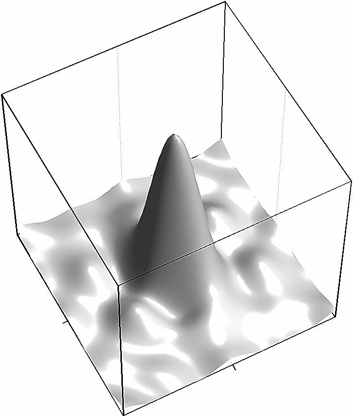
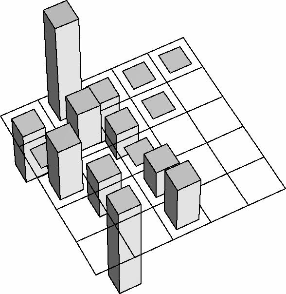
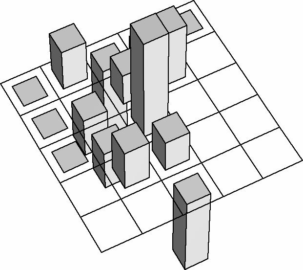
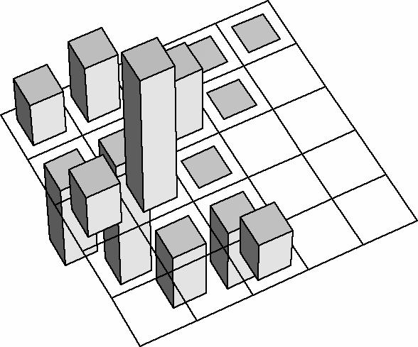
64 1.9. Conclusions to the chapter 47 DC element Orthonormal SA-DCT Figure 1.30: A complete orthonormal set of 15 SA-DCT basis elements and a DC (constant) element used for the mean subtraction (top). The respective Fourier-domain power spectrum is shown below each SA-DCT basis element and to the right of the DC element.

65 48 1. Pointwise Shape-Adaptive DCT denoising and deblocking facts are suppressed while salient image features are preserved. The luminancedriven shape-adaptive Þltering can faithfully reconstruct the missing structural information of the chrominances, thus correcting color-bleeding artifacts. The visual quality of the estimates is high, with sharp detail preservation, clean edges, and without unpleasant artifacts introduced by the Þtted transform. Moreover, this is achieved at a very competitive computational cost. Overall, the Pointwise SA-DCT Þltering algorithms demonstrate a remarkable performance, often outperforming all previous methods known to the authors.

66 Chapter 2 Pointwise SA-DCT regularized deconvolution In this chapter we extend the Pointwise SA-DCT denoising approach to image deblurring. First, let us generalize the observation model (1.1) given in Section 1.2, introducing an optical blurring into the observation process. This distortion is commonly modeled by the convolution y ~ v of the true image y with the pointspread function (PSF) v of the optical system. Thus, we wish to recover y from the blurred and noisy observations z (x) =(v ~ y)(x)+η (x), x X. (2.1) In the frequency domain the above equation becomes Z = YV + η, wherecapital letters are used for the discrete Fourier transform of the corresponding variables and η = F (η), η ( ) N 0, X σ 2. It is assumed that the PSF v is known. Note that the observation model (1.1) is a particular case of (2.1) where v is a Dirac function. The proposed deblurring algorithm is based on the anisotropic regularized inverse (RI) and regularized Wiener inverse (RWI) LPA-ICI deconvolution scheme developed in [94, 91]. The same deconvolution technique had also been used for inverse halftoning [56] and Poissonian deblurring [50]. The idea of the proposed SA-DCT domain deblurring is to combine the SA- DCT transform with the regularized inversion operators, using the adaptive supports deþned by the anisotropic LPA-ICI regularized deconvolution. The ßowchart of the overall deblurring algorithm is shown in Figure Regularized inverse The regularized inverse (RI) z RI is computed in the frequency domain as z RI = F 1 V (T RI Z), T RI = V 2 + ε 2, (2.2) 1 49

67 50 2. Pointwise SA-DCT regularized deconvolution Figure 2.1: Flowchart of the SA-DCT regularized Wiener inverse algorithm. In the upper part of the ßowchart a deblurred estimate ŷ RI is obtained by combining the regularizedinversion (RI) operator with the SA-DCT-domain hard-thresholding. This estimate is used as reference estimate for the regularized-wiener stage of the lower part of the ßowchart, where a regularized Wiener inverse (RWI) operator is combined with Wiener Þltering in SA-DCT domain. The intermediate ŷ RI and the Þnal ŷ RW I estimates are respectively obtained by averaging with adaptive weights (represented as Σ ) the local SA-DCT estimates ŷx RI and ŷx RW I, whose supports are deþned by the anisotropic LPA-ICI technique on the regularized inverse z RI and regularized Wiener inverse z RW I.Examples of the estimates obtained at the various stages of the algorithm are shown in Figure 2.2. where T RI is a (Tikhonov) regularized-inversion operator, ε 1 > 0 is a regularization parameter 1, and V is the complex conjugate of V. In what follows we make explicit use of the impulse response t RI of the regularized-inversion operator, t RI = F 1 (T RI ). 2.2 Adaptive anisotropic transform support The anisotropic neighborhood U x + is constructed from the adaptive scales {h + (x, θ k )} K k=1 obtained from the following procedure. The LPA is performed in the spatial domain as a convolution of the regularized inverse z RI against the LPA kernel g h,θk, öy h,θ RI k = z RI ~ g h,θk, for each speciþed direction θ k, k =1,...,K, and for every scale h H. All the varying-scale LPA estimates {öy h,θ RI k } h H obtained for each θ are fed (together with their standard deviations {σŷri = h,θ σ kt RI ~ g h,θ k 2 } h H ) into the ICI algorithm, which selects the pointwise-adaptive scale h + (x, θ k ). The adaptive scale selection is done independently for each direction θ k. 1 The regularized inverse estimate (2.2) corresponds to the least-squares problem with penalty on the / 2 norm of the estimate T RI Z =argmin Y kyv Zk ε2 1 ky k2 2. When ε 1 0, the regularized inverse converges to a pseudo-inverse, typically becoming unbounded.

68 2.3. Pointwise SA-DCT deblurring 51 z z RI z RW I ŷ RI ŷ RW I Figure 2.2: Examples of the estimates obtained at the various stages of the Pointwise SA-DCT regularized deconvolution algorithm (see also the ßowchart of the algorithm in Figure 2.1). The images correspond to the deblurring Experiment 3, described in Table 2.1. The ISNR of the ŷ RI and ŷ RW I estimatesis5.57and6.34db,respectively.observe the ampliþcation of the noise after the inversion of the blur. Some granularity typical of colored noise is also visible. The subimage at the bottom-right shows some of the anisotropic neighborhoods used as support for the SA-DCT in the Pointwise SA-DCT Wiener Þltering stage. Here H = {1, 2, 4}. 2.3 Pointwise SA-DCT deblurring A non-linear adaptive deblurring operator is obtained by combining the regularized inversion (2.2) with the shape-adaptive DCT domain shrinkage. While formally

69 52 2. Pointwise SA-DCT regularized deconvolution it is enough to replace z by z RI in (1.6), several further modiþcations to the basic denoising procedure of Section 1.5 are required in order to properly take into account the initial regularized inversion. The principal difference arises from the fact that, because of the blur inversion (2.2), the noise in z RI is colored. Therefore it is not possible anymore to guarantee that the noise variance in the SA-DCT domain is constant (as observed instead in Section 1.4.1). Because the noise variance can possibly vary signiþcantly from a transform coefficient to the other, a constant threshold like (1.7) cannot be used in order to determine which coefficients should be used for the reconstruction of the deblurred estimate. 2.4 Thresholding with adaptive variance in transform domain We consider the individual variance of the transform coefficients ϕ zri,x = TŨ + x (z RI Ũ + x mũ + x (z RI )) Let i VŨ + x be coordinates in SA-DCT domain and ψ (i) : Ũ U + x + x R the SA- DCT basis functions, as deþned in (1.12). Neglecting the correlating effect of the mean subtraction ( DC separation ), the variance σ 2 ϕ zri,x (i) of the i-th transform coefficient ϕ zri,x (i) is σ 2 ϕ zri,x (i) = σ 2 t RI ~ ψ (i) X 2 Ũ x + 2 = σ2 T X RI F(ψ (i) X ) 2 Ũ x + 2, (2.3) The appropriate threshold level for each transform coefficient is obtained by replacing the coefficient-invariant σ in the threshold (1.8) with the varying standard deviation σ ϕzri,x : VŨ + x R. In this way, we realize an adaptive hard-thresholding rule for the joint deblurring and Þltering in SA-DCT domain. Analogously to (1.6), a local deblurred estimate öy RI is obtained by inverse Ũ x + transformation of the thresholded coefficients. 2.5 Adaptive weights and global estimate Just as in Section 1.5.3, in order to obtain a global estimate öy RI the local estimates öy RI are averaged together using adaptive weights w Ũ x + x RI : X R all R in a convex combination analogous to (1.10). However, because of the different variances of the coefficients used in the reconstruction, the adaptive weights are deþned by a different formula. Ignoring the correlation between the noise in the transform domain, the corresponding expression of (1.11) for deblurring is 1 wx RI = ³ σ 2 m zri,x + P j S σ2 ϕ zri,x (j) U x +

70 2.6. Regularized Wiener inverse 53 where S VŨ + x and indicates the coefficients which are non-zero after thresholding σ 2 m zri,x = σ 2 t RI ~ χ Ũ x q + U x σ 2 = U T x + RI F(χŨ + X x ) 2 2 (2.4) is an extra term which accounts for the DC separation. In (2.3) we interpret the DC as calculated by a normalized basis element of the form χ Ũ x Ũ +, therefore x + var {m zri,x } = σ 2 m zri,x / U + x. 2.6 Regularized Wiener inverse The regularized Wiener inverse (RWI) z RW I is computed as z RW I = F 1 V Y 2 (T RW I Z), T RW I = VY 2 + ε 2, (2.5) 2 X σ2 where ε 2 > 0 is a regularization parameter 2. Since the spectrum Y 2 of the true image is unknown, the estimate öy RI from the RI stage is used quite naturally as a pilot estimate in the Wiener Þltering. It means that Y 2 in (2.5) is replaced by Y ö RI 2. Analogously to Section 2.2, the adaptive neighborhoods U x + are deþned by the anisotropic LPA-ICI technique applied to z RW I. On these neighborhoods we perform empirical Wiener Þltering in SA-DCT domain in a fashion similar to Section More precisely, for every x X, let ϕŷri,x : VŨ + x R be the SA-DCT (on U x + )coefficients of öy RI where the mean mũ + x (z RW I ) of z RW I is subtracted before applying the transform: ϕŷri,x = TŨ + x ³öy RI Ũ + x mũ + x (z RW I ). (2.6) The local Wiener estimate öy wi Ũ + x is deþned as öy wi Ũ + x = T 1 Ũ x + ωx ϕ zrw I,x + Nx mũ + x (zrw I ), (2.7) where the attenuation coefficients for this Þlter are ω x = ϕ 2 ŷri,x ϕ 2 ŷri,x + σ2 ϕ zrw I,x, N x = m 2 Ũ + x m 2 Ũ + x (öy RI ) (öy RI )+σ 2 m zrw I,x / U x +. 2 If ε 2 =1, the inverse operator! T RW I (2.5) " corresponds to the solution of the minimum MSE problem T RW I =argmin T E ktz Y k 2 2.Anε 2 6=1producesinverse operators with a balance between bias and variance different than the optimum one, obtained for ε 2 =1. In particular, the smaller is ε 2, the smaller is the bias and the larger is the variance (i.e. noise) in the inverse estimate z RW I. Since we are able to further suppress the noise exploiting the Pointwise SA-DCT Þlter, it is worth choosing ε 2 1. In this way we are able to achieve lower bias and in the end (after Pointwise SA-DCT Þltering) also lower variance (thus, lower MSE) than by the optimum Wiener inverse Þlter with ε 2 =1.

71 54 2. Pointwise SA-DCT regularized deconvolution The variances σ 2 ϕ zrw I,x and σ 2 m zrw I,x are deþned as in (2.3) and (2.4), but using the regularized Wiener inverse operator T RW I or its impulse response t RW I = F 1 (T RW I ) instead of T RI or t RI, respectively. These variances are also used to deþne the adaptive weights used for the aggregation of the local estimates (2.7): 1 wx RW I = ³N 2 xσ 2 mzrw I,x + P ω 2 VŨ+x xσ 2 ϕzrw I,x U. x Fast computation of coefficients variance The calculation of the variance of the transform coefficients as in (2.3) is a rather computationally intense procedure. In order to reduce complexity to an acceptable level, it is necessary to employ some approximations. Our implementation of (2.3) is based on processing in an undersampled (coarse) FFT domain of size Denoting by e F the corresponding transform, by e X a32 32 domain, and by L a decimator with preþltering, we have the following approximation of the variance of the i-th transform coefficient ϕ zri,x (i): σ 2 ϕ zri,x (i) ' σ2 X e L{ F(t RI ) 2 } F(ψ e (i) #X ) 2 Ũ x + 1, σ 2 σ 2 m zri,x ' U x + X e L{ F(t RI ) 2 } F(1 e #X Ũ x + ) 2 1. (2.8) An obvious modiþcation to the above formula allows to compute approximations of the variances σ 2 ϕ zrw I,x. Figures 2.3 and 2.4 show some SA-DCT basis functions ψ (i) and their corresponding power spectrum ef(ψ (i) #X ) 2, as used in (2.8). These Ũ x + Ũ x + examples, together with those in Figure 1.30, clearly show that the SA-DCT basis elements are well localized in the frequency plane. This property results in large differences in the variances σ 2 ϕ zri,x (i) when F(t RI ) is non-uniform (e.g., concentrated at particular frequencies). The approximations (2.8) have a signiþcant impact on the computational performance of the algorithm. On a 1.5-GHz Pentium M CPU, the current Matlab implementation can process a image in about 9 seconds and a image in about 38 seconds. This includes RI and RWI stages, comprehensive of LPA-ICI and transform-domain Þltering. If (2.3) were used instead of the approximate (2.8), the processing time would be of several minutes, without any noticeable improvement in the restoration quality. 2.8 Experiments In order to evaluate the restoration ability of the proposed deblurring algorithm, we consider the standard set of four blurred and noisy observations which has been used by many other authors. Table 2.1 presents the description of the observations parameters. The blur PSFs for these experiments are shown in Figure 2.5. Roughly speaking, these four experiments represent different combinations of

72 2.8. Experiments 55 # X 2 # Figure 2.3: Some SA-DCT basis elements ψ + and their power spectrum F(ψ ) + U x U x used in the fast computation of the coefficients variance (2.8). (i) (i) # X 2 # Figure 2.4: Some SA-DCT basis elements ψ + and their power spectrum F(ψ ) + U x U x used in the fast computation of the coefficients variance (2.8). (i) (i) blur and noise in a gradation from the strong blur with weak noise (comparable to quantization noise) of Experiment 1, to the mildly blurred image with noticeable noise of Experiment 4. The spectral characteristics of the blur PSFs used in the experiments can be seen in Figure 2.6. In the same Þgure, we show also the amplitudes T R I and T RW I of the Fourier-domain regularized inverse (2.2) and regularized Wiener inverse operators (2.5). The regularization parameters ε1 and ε2 have been chosen manually for each experiment3. For calculating the SA-DCT coefficients variance (2.8), we use the downsampled L{ T R I 2 } and L{ T RW I 2 }, 3 Adaptive procedures for the automatic selection of the regularization parameters can also be utilized (e.g., [121], [178], [162]).

73 56 2. Pointwise SA-DCT regularized deconvolution Exp. Image, Point-Spread Function v, noise 1 Cameraman BSNR= 40dB 9 9 boxcaruniformv (σ 2 ' 0.308) 2 Cameraman σ 2 =2 v (x 1,x 2 )=1/ 1+x x2 2, x1,x 2 = 7,...,7 3 Cameraman σ 2 =8 v (x 1,x 2 )=1/ 1+x x2 2, x1,x 2 = 7,...,7 4 Lena σ 2 =49 v =[1, 4, 6, 4, 1] T [1, 4, 6, 4, 1] /256 Table 2.1: Description of the observation parameters for the four deblurring experiments. Exp. 1 Exp. 2 & Exp. 3 Exp. 4 Figure 2.5: Point-spread functions v for the four deblurring experiments of Table 2.1. The amplitude of the Fourier transform of these PSFs is illustrated in Figure 2.6. showninfigure2.7. Moreprecisely,weintegratethepointwiseproductofthe power spectrum F(ψ e (i) #X ) 2 (shown in Figures 2.3 and 2.4) with the downsampled power spectrum of the noise L{ F(t RI ) 2 } (whose root is shown in Figure 2.7) Ũ x + or L{ F(t RW I ) 2 }. As already mentioned, the standard-deviation can vary signiþcant from a coefficient to the other. For example, at the RI stage of Experiment 4 and for the same anisotropic support of the basis functions shown in Figure 2.4, the computed standard deviations of the SA-DCT coefficients and of the mean are σ ϕzri,x = σ mzri,x = The improvement-in-snr (ISNR) results for these four experiments are given in Table 2.2. Figure 2.8 show details of the observations and the corresponding restored images. Similarly to denoising, both the objective and subjective quality of our estimates are high. In the case of deblurring, the Pointwise SA-DCT is particularly effective in coping with the ringing artifacts due to the regularization of the inverse operator. To the best of our knowledge, on these standard experiments, the proposed Pointwise SA-DCT regularized deconvolution outperforms all other methods to date.

74 2.8. Experiments 57 V T R I T RW I V T R I T RW I V T R I T RW I V T R I T RW I E X P. 1 E X P. 2 E X P. 3 E X P. 4 Figure 2.6: Amplitude of the Fourier transform V of the PSF v and of the regularized inverse and Wiener inverse operators T R I and T RW I for each of the four deconvolution experiments (Section 2.8).

75 58 2. Pointwise SA-DCT regularized deconvolution Figure 2.7: Square root of the downsampled power spectrum of the noise $ $ for the regularized inverse, L{ F(tR I ) 2 }, and for the regularized Wiener inverse, L{ F(tRW I ) 2 }, in each of the four deconvolution experiments (Section 2.8). These power spectra are used in (2.8). Compare with the corresponding undecimated functions in Figure 2.6. Method Experiment 1 Pointwise SA-DCT regularized deconvolution 8.57 Anisotropic LPA-ICI RI-RWI [91, 62] 8.29 BOA (Figueiredo and Nowak) [46] 8.16 GEM (Dias) [34] 8.10 Segmentation-based regularization (Mignotte) [115] 8.04 EM (Figueiredo and Nowak) [45] 7.59 ForWaRD (Neelamani et al.) [121] Table 2.2: ISNR (db) of the proposed deblurring algorithm and of other state-of-the-art methods for four standard experiments. 2.9 Some comments on the approach Let us give some comments and discussion of the general nature on the deconvolution approach used for the two stages of our algorithm. n o (i) ª ù Given a frame ψ (i) and its dual ψ, we can represent the original signal i i using the usual analysis-synthesis form y= X i ù y, ψ (i) (i) ψ. (2.9) Let us now be given not y but its blurred (noise-free) observation y ~ v. There are essentially two strategies which can be followed starting from Equation (2.9).

76 2.9. Some comments on the approach 59 Figure 2.8: From top to bottom: fragments of the observations z and of the corresponding Pointwise SA-DCT estimates ŷ RW I of four deblurring experiments. The ISNRs of these estimates are 8.57, 8.25, 6.34 and 4.52 db, respectively.

77 60 2. Pointwise SA-DCT regularized deconvolution Synthesis with ψ (i)ª i We would like to reconstruct y using the frame elements ψ (i) in the form y = X i c iψ (i), (2.10) where the coefficients c i are computed from y ~ v. Obviously, c i = y, ψ ù (i) is a solution of the equation (and is the unique solution if the frame is a basis). For a generic y, the problem can be formally solved under the often unrealistic hypothesis that the blur operator is invertible. In this case we have that y, ψ ù (i) 1 D = F (y), F ù (i) E ψ = 1 D E YV, F(ù ψ (i) ) = (2.11) X X V D = y ~ v,f 1 F( ψ ù (i) ) E = (2.12) V D = y ~ v, ψ ù (i) ~ F 1 E 1, (2.13) V where V is the complex conjugate of V.Sothecoefficients c i can be calculated as the inner product between the blurred observations and ψ ù (i) ³ ~ F 1 1. V Analysis with ù ψ (i)ªi An alternative approach to (2.10) is to seek a solution of the form y = X i y ~ v, ù ψ (i) ξ (i), (2.14) where the true signal is analyzed with respect to the dual frame ψ ù n (i)ªi and synthesized with an appropriate set of reconstructing functions ξ (i)o. In order n i to get an explicit form for ξ (i)o we convolve the left and right-hand side of the i above equation against v, obtaining y ~ v = X y ~ v, ù (i) ψ ξ i (i) ~ v. (2.15) n o This perfect reconstruction formula implies that ξ (i) ~ v is a dual frame of i ùψ (i)ª i. For example, ξ(i) ~ v = ψ (i), which gives (assuming invertibility of V ) ξ (i) = F 1³ F(ψ (i) ) V. (2.16) Ill-posedness and regularization Usually, blur operators are not invertible. In the case V has zeros, the simplest ( naïve ) approach is to use a generalized inverse of V, i.e. ½ V 1 0 if V ( ) =0 ( ) = 1/V ( ) if V ( ) 6= 0.

78 2.9. Some comments on the approach 61 However, even when V does not have zeros, the problem can still remain ill-posed, with the inverse operator V 1 being unbounded. Consequently, when approaching noisy observations of the form (2.1), the typical strategy is to employ regularization at some stage of the inversion procedure. The simplest form of regularization is the following (Tikhonov) regularized inverse [168],[40] V T RI = V 2 + ε 2, (2.17) where ε>0 is the regularization parameter. A larger regularization parameter corresponds to a more stable (lower variance) but also more biased inverse estimate. The regularization (2.17) has been used extensively for deblurring, in the spatial domain (e.g., [10], [91], [94], [50], [168]), as well as in the transform domain (e.g., [121], [53]). Similar forms of regularization combined with transform-domain Þltering can be found also in [7] and [120]. In all these approaches, the combination of Fourier-domain regularization with other Þltering techniques (e.g., adaptive smoothing, shrinkage, etc.) is shown to lead to an improved inverse estimate Intermediate cases; comments; vaguelettes In addition to the two strategies from Sections and 2.9.2, there are also inþnitely many intermediate cases. Exploiting in (2.9) the fact that formally y, ψ ù (i) D = 1 X YV α, F ψ ù (i) E n o α V, it is easy to show that ψ (i) ~ F 1 (V α ) n ³ i and ùψ (i) α o ~ F 1 V are also a pair of frames in duality, for any α R. i By using this new pair of frames instead of nψ (i)o and ù (i)ª ψ in (2.10) and by i i varying α, one can obtain the Þrst (α =0) and the second strategy (α =1), all intermediate cases (0 <α<1), as well as other decompositions (α <0, α>1). Although the two approaches might seem formally equivalent, they become in practice very different as soon as they are considered with respect to a predeþned meaningful frame. n Equation (2.10) implicitly assumes that ψ (i)o is a suitable frame to enable i a good approximation of y. Since the inverse operator is embedded in the analysis frame, the approach works according to the paradigm Þrstinverttheblur, and is suitable to approxi- n ξ (i)o. i then approximate this inverse. n On the contrary, Equation (2.14) assumes that ψ (i)o i mate y~v, with the inverse operator embedded in the reconstruction frame Thus, it essentially obeys to the paradigm Þrst approximate the blurred signal, and then invert this approximation. If not all coefficients are used for the reconstruction, the two approaches lead to signiþcantly different approximations of y. In our work, we consider frames corresponding to redundant shape-adaptive DCT transforms deþned on pointwise adaptive starshaped domains. Redundancy (overcompleteness) comes from the fact that multiple overlapping starshaped domains are used and that for each such domain a complete SA-DCT transform is

79 62 2. Pointwise SA-DCT regularized deconvolution n computed. Originally, this deconvolution approach was studied with ψ (i)o and i ùψ (i)ª being biorthogonal wavelet bases: the representations (2.10) and (2.14) are i respectively known within the wavelet community as wavelet-vaguelette [35, 107] and vaguelette-wavelet [1] decompositions. Vaguelette stands for the combination of the inverse of the blur with the corresponding dual wavelet, such as ξ (i) from (2.16). We refer the reader to [1] for a theoretically-oriented discussion and comparison of the asymptotical risk of estimators based on the two approaches. Letusnotethattheframe nψ (i)o and its dual ù (i)ª ψ i interchanged in all the above equations Practical aspects i can be obviously Pragmatically, if to be used in estimation from noisy observations, each one the two approaches has its own advantages and disadvantages. In particular, assuming a properly normalized frame and independent noise with constant variance, shrinkage of coefficients which are calculated directly from the blurred observations as in (2.15) is simpliþed. Note that (diagonal) shrinkage requires the knowledge of the standard-deviation of each coefficient, which can be calculated according to thesimpleformula std {hf,gi} = r D var {f}, g 2E, provided the independency of the noise in f. If var {f} is also constant, say, var {f} = σ 2,then std {hf,gi} = σ kgk 2. (2.18) Thus, as far as coefficient shrinkage is concerned, the approach is very similar to transform-based denoising from standard Gaussian noise. On thenother hand, the convolution against the (regularized) inverse of V can cause that ξ (i)o does not n i enjoy any of the good decorrelation properties of the original frame ψ (i)o.thus, i the approximation ability of the approach (2.14) can be seriously impaired. In (2.10) the original frame is used for reconstruction, however, even in the simplest case of noise with constant variance, the shrinkage of coefficients obtained by (2.13) is rather involved because the combination of dual frame with the inverse operator. Nevertheless in practice, since the main motivation to use a transform-based method is its ability of to represent the signal to be recovered with good approximation by using only few transform coefficients (i.e. sparsity), the approach from Section is more appropriate, despite the calculation of the standard-deviation (required for the shrinkage) is usually more involved Decoupling of the transform and the inversion As mentioned in Section 2.9.4, Equation (2.10) works according to the paradigm Þrst invert the blur, and then approximate this inverse.

80 2.9. Some comments on the approach 63 D E If in the term YV, F(ù ψ (i) ) from (2.11) we replace the noise-free data YV V with Z and the naive inverse 1 V with a regularized inverse (2.17), we obtain that the coefficients c i are calculated as 1 X DZ, F ù ψ (i) E V V 2 +ε 2 1 D = Z V X V 2 +ε, F ù (i) E ψ = 2 = z RI, ψ ù (i), ³ where z RI = F 1 ZV V 2 +ε is the regularized-inverse estimate of y. Although, 2 in principle, different forms of regularization (e.g., different regularization parameters) could be used for different coefficients, for computational reasons it is preferable to use a unique regularized inverse z RI for all i. Inthiswaythecalculation of the inner products is done exactly as for the analysis of z RI with the frame ùψ (i)ª. Thus, we come to the following approximation of y in terms of the frame n i ψ (i)o i y ' X i z RI, ù ψ (i) ψ (i). The coefficients z RI, ψ ù (i) are noisy and some shrinkage should be performed in order to obtain a good estimate. The noise in z RI is not white, but colored through inverse Þltering with T RI (2.17), thus the thresholds used in the shrinkage are different for different coefficients. n In order for this shrinkage to be effective it is important that the frame ψ (i)o represents well y. The redundant shape-adaptive i n DCT transform on adaptive supports is thus an excellent choice for ψ (i)o when i natural images are considered as the original signal to be reconstructed 4. Finally,theestimatehasthegenericform X öϕ (i) i ψ(i), (2.19) where öϕ are the Þltered coefficients obtained by shrinkage (e.g., hard-thresholding) of z RI, ψ ù (i) Global Fourier-domain inverse, periodicity, and localized processing In our approach, we explicitly use the impulse response t RI of the regularizedinversion operator, t RI = F 1 (T RI ). The inversion (2.2) is naturally computed globally, assuming periodicity of the processed signal and of the convolutions used in the corresponding space-domain operations. Obviously, such modeling does not 4 When comparing these equations with those from Section 1.5.3, one should observe that the role of ψ ù (i) and ψ (i) is reversed, as the emphasis is placed on two different parts of the analysisreconstruction paradigm. Here, we Þx the reconstruction frame, whereas there is the analysis frame that is Þxed. Overall, the aim is to reconstruct the deblurred signal using the same frame used for denoising.

81 64 2. Pointwise SA-DCT regularized deconvolution correspond to the reality, as the translation-invariant blur due to optics or rigid motion does not make the signal periodic. The application of the inverse (2.2) on anon-periodicz results in dramatic boundary artifacts, which often may cause the whole estimate to be degenerate. However, there are a number of efficient sectioning techniques (e.g., [3], [142]) which enable the proþtable useofthein- verse (2.2) on non-periodic signals. The key idea of these techniques is to force z to be periodic, replacing its original non-periodic boundaries with synthesized smoothed periodic boundaries (a procedure called apodization of the image). In a similar way, this allows to process large images in a localized or windowed fashion (which is necessary when severely limited memory or computational power is available). Whenever t RI has a fast enough decay, such sectioning techniques can be used without producing any visible distortions. Clearly, the same considerations as above apply to the regularized Wiener inverse (2.5) also Extensions The proposed deblurring algorithm can be easily extended to observation models more general than (2.1). In particular, we refer the reader to [31], where a straightforward modiþcation of the algorithm a modiþcation that permits the noise η to be colored instead of white, as in (2.1) is exploited for inverse-halftoning of errordiffused binary-halftone images.

82 Chapter 3 Signal-dependent noise removal This chapter presents a novel and efficient method for denoising of images corrupted by signal-dependent noise based on shrinkage in the shape-adaptive DCT (SA-DCT) domain. The use of an adaptive transform support enables both a simpler modelling of the noise in the transform domain and a sparser decomposition of the signal. Consequently, coefficient shrinkage is very effective and the reconstructed estimate s quality is high, in terms of both numerical error-criteria and visual appearance, with sharp detail preservation and clean edges. Simulation experiments demonstrate the superior performance of the proposed algorithm for a wide class of noise models with a signal-dependent variance, including Poissonian (photon-limited imaging), Þlm-grain, and speckle noise. 3.1 Introduction In many applications the observed signal is corrupted by a signal-dependent noise. The most widely encountered models are Poisson, Þlm-grain, multiplicative, and speckle noise. Their common feature is that the variance of the noise is directly related to the true-signal s intensity. In particular, because of the inherent photoncounting process within digital imaging sensors, the noise found in digital images is signal-dependent, with brighter parts of the image having a larger noise variance, and typically following a Poissonian distribution. These aspects will be discussed more in detail in the second part of the thesis. Starting with classical Þlters, such as those by Lee, Kuan, and Frost ([105], [106], [103], [66]), a number of adaptive approaches for signal-dependent noise removal have been developed and proposed, in spatial (e.g., [87], [140], [51]) as well as in transform domain (e.g., [164], [173], [111], [52]). In this chapter, we extend the Pointwise SA-DCT denoising Þlter, introduced in Chapter 1, to the Þltering of signal-dependent noise. Also in this case, denoising is performed by coefficient shrinkage in the SA-DCT [154] domain, with the Anisotropic Local Polynomial Approximation (LPA) - Intersection of ConÞdence 65

83 66 3. Signal-dependent noise removal Intervals (ICI) technique [91, 92] used to deþne the shape of the transform s support in a pointwise adaptive manner. On such adaptive supports the signal is smooth and nearly constant, allowing for a simpler modelling of the noise within each transform support and enabling a sparser decomposition of the signal in the transform domain. Thus, coefficient shrinkage (e.g., hard-thresholding and Wiener Þltering) can be employed directly, accurately, and very effectively. As a result, the reconstructed estimate s quality is high, in terms of both numerical errorcriteria and visual appearance. In particular, thanks to shape-adaptive transform supports, the estimates exhibit sharp detail preservation and clean edges. The key element of our approach to signal-dependent noise is the use of a locally adaptive estimate of the noise variance, an estimate which is progressively reþned during the various stages of the algorithm. The presented method generalizes and extends both the Pointwise SA-DCT Þlter for denoising of additive white Gaussian noise (AWGN) [58], presented in Chapter 1, and the Adaptive-Size Block-DCT (AS B-DCT) algorithm [52] for signal-dependent noise removal with adaptive-size block transforms, recently proposed by the authors. The rest of the chapter is organized as follows. In the next section we introduce the general signal-dependent noise model and the notation used throughout the chapter. The algorithm is then presented in detail: construction of the adaptiveshape support, hard-thresholding in SA-DCT-domain, aggregation of overlapping local estimates, and empirical Wiener Þltering in SA-DCT domain. The last section of the chapter is devoted to experimental results for removal of Poissonian (photon-limited imaging), Þlm-grain, and speckle noises. 3.2 Signal-dependent noise model We consider observations z(x), x X Z 2, with the expectations E{z(x)} = y(x) 0, where the errors (noise) η (x) =z (x) y (x) are independent and the variance of these observations is modeled as σ 2 z (x) =var{z(x)} =var{η(x)} = ρ(y(x)), (3.1) ρ : R + R + being a given positive function of y called the variance function. For example, ρ(y) =y, ρ(y) =y 2,andρ(y) =(Ky α ) 2 for the Poisson, gamma, and Þlm-grain observation models, respectively. The problem is to reconstruct the true image y from the noisy observations z. 3.3 Algorithm Similar to the algorithm for AWGN presented in Section 1.5, the following algorithm for signal-dependent noise comprises two stages: a Þrst stage (Sections ) based on hard-thresholding, and a second stage (Sections ) based on empirical Wiener Þltering, where the hard-thresholding estimate obtained in Section is used as a reference estimate. The Þrst step in each stage employs the Anisotropic LPA-ICI technique [47, 91, 92] in order to identify adaptive neighborhoods where the image can be assumed to be locally smooth (polynomial Þt) and nearly constant.

84 3.3. Algorithm 67 Figure 3.1: LPA-ICI anisotropic neighborhoods. Left: some examples of the anisotropic neighborhoods Ũ x + used for SA-DCT Þltering of the Peppers image corrupted by Poissonian noise (χ=0.1). Right: the corresponding cross-sections (column 87) of the true image y, of the noisy observation z, and of the Pointwise SA-DCT estimate ŷ wi. The signal-dependent nature of the noise is clearly visible Stage 1: Hard-thresholding in Pointwise SA-DCT domain Adaptive-shape neighborhood We initialize the algorithm with a simple, rough estimate öσ 2 z of the variance σ 2 z obtained as the variance function evaluated on the noisy data, öσ 2 z = ρ ( z ). For every speciþed direction θ k, k =1,...,K, a varying-scale family of 1-D directional-lpa convolution kernels {g h,θk } h H is used to obtain a corresponding set of directional varying-scale estimates {öy h,θk } h H, öy h,θk = z ~ g h,θk, h H, where H R + is the set of scales. For these 1-D kernels, the length of the support coincides with the value of the scale. The qpointwise standard-deviations of the estimates öy h,θk are estimated as öσŷh,θk = öσ 2 z ~ gh,θ 2 k, h H. Thus, for each point (pixel) x X we obtain a sequence of conþdence intervals nh io öy h,θk (x) Γöσŷh,θk (x), öy h,θk (x)+γöσŷh,θk (x) where Γ is a positive threshold parameter. These intervals are then compared according to the ICI rule [72, 90], and as a result an adaptive scale h + (x, θ k ) H is deþned for every x X. Precisely, the adaptive h + (x, θ k ) is deþned as the largest scale h such that the intersection of all conþdence intervals corresponding to scales smaller than h is non-empty. The procedure is repeated for all speciþed directions. Thus, for a Þxed x X we have K directional adaptive scales h + (x, θ k ),k= 1,...,K. In our implementation, like in Section 1.5.1, we use K =8directions and construct the adaptive neighborhood U x + of x as U x + = {v X :(x v) U x + }, where U x + is the polygonal hull of the supports of the adaptive-scale kernels ª 8 gh + (x,θ k ),θ k. Figure 3.1(left) shows some examples of these neighborhoods k=1 for a noisy image corrupted by Poissonian noise. Observe how these neighborhoods h H

85 68 3. Signal-dependent noise removal adapt to edges and variations in the image intensity and that in each neighborhood the underlying image is smooth and nearly constant. Hard-thresholding in SA-DCT domain: local estimates For every neighborhood U x +, x X, weconstructalocal estimate öyũ + x : U x + R of the signal y by hard-thresholding in SA-DCT domain. The typically encountered variance functions ρ, such as those mentioned in Section 3.2, are smooth functions of their argument y. As a consequence, on neighborhoods where the signal is nearly constant, so is its variance. It means that with a good approximation, the variance can be assumed to be constant when the transform s support is restricted to a region of signal uniformity such as the adaptive neighborhood U x +. Thus, locally, the hard-thresholding can be performed as in the standard case [58] where³ the variance is everywhere constant, provided that a locally adaptive estimate öσ 2 z U x + of the variance of the noise in U x + is used. ³ Such a locally adaptive öσ 2 z U x + can be obtained from the mean mũ + x (z) ³ through the variance function as öσ 2 z U + x = ρ ³ mũ + x (z). For any given neighborhood U x +, this adaptive variance is a constant. Hence, similar to ( ), the local estimate öyũ + x is calculated as öyũ + x = T ³Υ 1 Ũ x + x ³TŨ ³z +x Ũ +x m +x Ũ (z) + mũ + x (z), (3.2) where Υ x is a hard-thresholding operator with adaptive threshold γ thr röσ 2 z ³ ³ U + x 2ln U x + +1, γ thr > 0, (3.3) This threshold is again Donoho s universal threshold (1.8), with the same Þxed parameter γ thr > 0. However, ³ here, instead of an invariant σ 2,weusethelocally adaptive variance estimate öσ 2 z U + x. Global estimate as aggregation of local estimates The Anisotropic LPA-ICI provides an adaptive neighborhood U x + for every x X. Neighborhoods corresponding o to adjacent points are usually overlapping, thus the local estimates nöyũ (3.2) constitute an overcomplete representation of the +x x X image. In order to obtain a single global estimate öy : X R deþned on the whole image domain, all the local estimates (3.2) are averaged together using adaptive weights w x R in the following convex combination: öy = Px X w xöyũ +x X Px X w xχũ +x. (3.4) Analogously to Section 3.3.1, the weights w x depend on the total sample variance of öyũ + x thus, on the number Nx har of non-zero coefficients after thresholding and

86 3.3. Algorithm 69 on the local variance öσ 2 z ³ U + x and on the size of the neighborhood U + x : w x = ³ öσ 2 z U x + (1 + Nx har ) U x +. (3.5) Stage 2: Wiener Þltering in Pointwise SA-DCT domain Improved adaptive-shape neighborhood Theestimateofthevarianceöσ 2 z used in Section (calculated from z through the variance function ρ) is indeed rough. A better estimate öσ 2 z can now be calculated from the above öy as öσ 2 z = ρ ( öy ). The Anisotropic LPA-ICI approach is used once more to deliver more accurate adaptive scales. We modify slightly the procedure from Section 3.3.1, in that the LPA estimates {öy h,θk } h H are now calculated not from z but from öy (3.4), as the convolution öy h,θk =öy~g h,θk, h H. Thestandarddeviations needed qfor the construction of the conþdence intervals are calculated again as öσŷh,θk = öσ 2 z ~ gh,θ 2 k, h H, withöσ 2 z = ρ ( öy ). As a result of the ICI rule, we obtain, for each x X, the new directional adaptive scales h + (x, θ k ), k =1,...,K, and thus the corresponding adaptive-shape neighborhood U x +. Wiener Þltering in SA-DCT domain: local estimates Using the estimate öy (3.4), the empirical Wiener Þlter in the SA-DCT domain worksasfollows. ForaÞxed x, letϕ z,x : VŨ + x R and ϕŷ,x : VŨ + x R be, respectively, the SA-DCT (on U x + )coefficient of z and öy, calculatedas ³ (z) ϕ z,x = TŨ + x z Ũ x + m Ũ x +, (3.6) ³ (z) ϕŷ,x = TŨ + x öy Ũ x + m Ũ x +, (3.7) where the mean mũ + x (z) of z is subtracted before applying the transform. The local Wiener estimate öy wi is deþned as Ũ x + öy wi = T 1 Ũ x + Ũ x + ωx ϕ z,x + Nx mũ + (z), (3.8) x where ω x VŨ + x and N x R are respectively the Wiener attenuation factors for ϕ z,x and for the subtracted mean value mũ + x (z), ϕ2 ŷ,x ω x = ϕ 2 ŷ,x +, N x = σ2 x m 2 Ũ + x m 2 (öy) Ũ x + ³ (öy)+öσ 2 z U + x / U, (3.9) x + ³ and öσ 2 z U + x is a local adaptive estimate of the variance of z in U x + calculated as ρ ³ mũ + (öy). x

87 70 3. Signal-dependent noise removal Final global estimate as aggregation of local estimates The global estimate öy wi can be obtained analogously as in (3.4), using the convex combination with the adaptive weights w wi öy wi = Px X wwi x : x öy wi X Ũ x P +, w wi x X wwi x χũ + x x = ³ öσ 2 z U + x (N 2 x + P ω 2 VŨ+ x) U x +. (3.10) x ³ Similarly to (3.5), the term öσ 2 z U + N 2 x x + P ω VŨ + x 2 in the adaptive weights x corresponds to an estimate of the total sample variance of öy wi. Ũ x + The Pointwise SA-DCT results which we present in this chapter correspond to the öy wi estimate (3.10) Complexity Thepresentedmethodforsignal-dependentnoiseremovalinheritsthesamelow computational complexity of the standard Pointwise SA-DCT developed for AWGN (Section 1.8.5). In fact, the extra operations in this generalized algorithm are essentially only the convolutions needed to calculate öσŷh,θk,andtheanisotropic LPA-ICI in the second stage of the algorithm. Both are computationally negligible compared to the multiple forward and inverse SA-DCT transforms performed ³ in Sections and The locally adaptive variance estimates öσ 2 z U + x are also calculated almost for free, since the local means mũ + x (z) and mũ + x (öy) are anyway required by standard algorithm for AWGN (in order to accomplish the DC separation). 3.4 Experimental results We show experimental results for three common types of signal-dependent noise: the scaled Poisson noise, χz P (χy),χ R +, χ 6= 0,thegeneralized Þlmgrain noise, z = y +(K 0 + K 1 y α ) η, K 0,K 1,α R + and η ( ) N (0, 1), and the multiple-look speckle noise, z = L 1 P L i=1 y`i, `i E (β), β R +, β 6= 0. The calligraphic letters P, N, ande denote, respectively, the Poisson, Gaussian, and exponential distributions. For the above observation models, the variance functions ρ (y) =σ 2 z are ρ (y) =y/χ, ρ (y) =(K 0 + K 1 y α ) 2,andρ(y) =y 2 β/l, respectively. The true signal y is assumed to have range [0,255]. Firstly, in Table 3.1 we give a comparison for the simulations presented in [140] for the above noise models with parameters χ=0.1, K 0 =0, K 1 =3.3, α=0.5, L=4, and β=1. In the table our results are compared against the adaptive-neighborhood Þlter [140], the noise-updating repeated Wiener Þlter [87] (as quoted in [140]), the recursive anisotropic LPA-ICI technique [51, 62], and the AS B-DCT algorithm [52]. Next, in Table 3.2 we compare our results for removal of Poissonian noise (χ = , , , ) against those obtained by two other transform-based methods [164],[111] recently developed speciþcally for this type of noise, by the

88 3.4. Experimental results 71 noise type noisy [87] [140] [51, 62] [52] P. SA-DCT Poisson (χ=0.1) Film-grain Speckle Poisson (χ=0.1) Film-grain Speckle Table 3.1: MSE results for different noise types and denoising algorithms. χ noisy [164] [111] [51, 62] [52] P. SA-DCT 30 / / / / / / / / Table 3.2: MSE comparison against algorithms for Poissonian noise. recursive anisotropic LPA-ICI technique [51, 62], and by the AS B-DCT algorithm [52]. The results in the tables show that the proposed algorithm outperforms all other methods, for all considered noise models and noise levels. In terms of MSE, the improvement is signiþcant especially for higher noise. Figures 3.2 and 3.3 provide a demonstration of the visual quality of the proposed Pointwise SA-DCT technique. Edges and small details are restored quite sharply, with very few noticeable artifacts. Figure 3.3 presents also a comparison between denoised estimates obtained by the AS B-DCT and by the Pointwise SA- DCT algorithms. Although the numerical difference is marginal, the two estimates are visually quite different. The AS B-DCT estimate has visible artifacts in the vicinity of sharp edges, and especially along the diagonal ones; the Pointwise SA- DCT estimate presents instead clean-cut edges that are comparable with those of the original image (shown in Figure 3.3(top-left)), thanks to superior spatial adaptivity. Finally, we compare our Pointwise SA-DCT against the TLS algorithm [78], which is developed to deal with observations of the form z = y +(K 0 + K 1 y) η, K 0,K 1 R + (i.e., one of the above models, with Þxed α =1). In Tables 3.3 and 3.4 we present PSNR and SSIM [172] results for K 0 =25, K 1 =0.1 and for K 0 =25, K 1 =0.2, respectively. The Pointwise SA-DCT achieves the best results on all images, with the notable exception of Barbara, to which apply the same considerations made in Section Figure 3.4 provides an illustration of the visual quality of the estimates. In the Þgure one can see that the Pointwise SA-DCT estimates are sharper and with fewer visible artifacts.

89 72 3. Signal-dependent noise removal Pointwise SA-DCT TLS (Hirakawa & Parks) [78] Lena Boats Barbara House Peppers 512x x x x x Table 3.3: PSNR (db, in regular type) and SSIM index [172] (in italic type) comparison table for the denoising of images with signal-dependent noise, where the observations have the form z = y +(25+0.1y)η, η( ) N (0, 1). Pointwise SA-DCT TLS (Hirakawa & Parks) [78] Lena Boats Barbara House Peppers 512x x x x x Table 3.4: PSNR (db, in regular type) and SSIM index [172] (in italic type) comparison table for the denoising of images with signal-dependent noise, where the observations have the form z = y +(25+0.2y)η, η( ) N (0, 1). Illustrative examples of denoising raw-data of digital imaging sensors are presented at the end of this thesis. We remark that the proposed method based on locally adaptive variance estimates is superior to the simpler approach where the noisy observations are preprocessed by a non-linear variance-stabilizing transformation (see, e.g., [139]) and then Þltered by an algorithm for AWGN. In particular, let us consider the Poissonian noise case and the procedure where the Anscombe transformation [5] is employed to stabilize the variance and denoising is then performed by the Pointwise SA-DCT algorithm [58] for AWGN (presented in Section 1.5), followed by inverse Anscombe transformation. For this simpler approach the MSE results are as follows: χ = 0.1 Peppers MSE=103, Aerial MSE=153; χ = 30/255 Lena MSE=59, Cameraman MSE=105. A comparison with the Tables 3.1 and 3.2 shows the improvement achieved by the use of locally adaptive variances. 3.5 Deblurring of images corrupted by signal-dependent noise As a Þnal remark, we note that the denoising algorithm presented in this chapter can be combined with the deconvolution approach from Chapter 2, resulting in a deblurring algorithm for images corrupted by signal-dependent noise. We refer the reader to our publication [49], where we present a similar procedure based on the block-dct with adaptive block-size.

90 3.5. Deblurring of images corrupted by signal-dependent noise 73 Figure 3.2: Peppers image (left), from top to bottom: original image, noisy observation corrupted by speckle noise (MSE=4442, PSNR=11.6dB), and Pointwise Shape-Adaptive DCT estimate ŷ wi (MSE=193, PSNR=25.3dB). Aerial image (right), from top to bottom: original image, noisy observation corrupted by Þlm-grain noise (MSE=829, PSNR=18.9dB), and Pointwise Shape-Adaptive DCT estimate ŷ wi (MSE=142, PSNR=26.6dB).

91 74 3. Signal-dependent noise removal Figure 3.3: Cameraman image. Left column, from top to bottom: original image, noisy observation corrupted by Poissonian noise (χ =30/255, MSE=1015, PSNR=18.1dB), and Pointwise Shape-Adaptive DCT estimate ŷ wi (MSE=100, PSNR=28.1dB). Right column, middle: noisy observation corrupted by Poissonian noise (χ =60/255, MSE=504, PSNR=18.1dB); top: AS B-DCT estimate [52] (MSE=70, PSNR=29.7dB); bottom: Pointwise Shape-Adaptive DCT estimate ŷ wi (MSE=68, PSNR=29.8dB).

92 3.5. Deblurring of images corrupted by signal-dependent noise 75 Figure 3.4: Top: noisy Peppers image, z = y+(25+0.1y)η, and noisy Barbara (fragments shown), z = y +(25+0.2y)η, η( ) N (0, 1). Center: TLS [78] estimates. Bottom: Pointwise SA-DCT estimates. The corresponding PSNR and SSIM results are given in Tables 3.3 and 3.4.

93 76 3. Signal-dependent noise removal

94 Chapter 4 Shape-adapted bases by orthonormalization The shape-adaptive DCT proposed by Sikora et al. can be implemented very efficiently with a negligible computational overhead with respect to the usual separable 2-D DCT on a rectangular support. However, for video-coding applications Gilge s shape-adapted DCT [70, 71] based on orthonormalization with respect to shape is known to achieve superior results than the approach by Sikora et al. It is considered [155] as a kind of upper bound on the decorrelation ability of the faster method. Thus, if computational complexity is not of primary concern, Gilge s method may be utilized as an alternative method to achieve further improvement in denoising. 4.1 Construction of a shape-adapted basis We remark that the implementation of such shape-adapted bases is not trivial. If general enough shapes are allowed 1, precalculation of all possible shape-adapted bases is not feasible because the resulting look-up-table would be huge. Hence, the orthogonalization must be performed on-line. There are two more problems. First, when restricting a basis to a region smaller than the initial domain of its elements, linear independence is certainly lost. This makes orthonormalization ill-posed. Second, the resulting shape-adapted orthonormal basis signiþcantly depends on the order in which the initial elements are orthonormalized. In particular, since an increasing number of orthogonal complements are successively subtracted during the orthogonalization, the similarity (and thus the common decorrelating features) between the resulting orthonormal elements and the initial ones diminishes as the procedure progresses. The combination of these two problems can have a devastating impact, because the attempt to orthonormalize any linearly-dependent element results in a systematic introduction of ampliþed 1 In our implementation for example despite the rather simpliþed neighborhood structure (based on H =6scales and K =8directions, as described in Figure 1.7), a total of 6 8 = different shapes are possible. 77

95 78 4. Shape-adapted bases by orthonormalization rounding-errors in all subsequent elements, which are thus distorted. A rather profound study of these problems, for the case of cosine and polynomial bases, is given in [131], providing criteria for the pruning of the starting basis so to obtain a set of elements which are linearly independent on the smaller region. Unfortunately, such criteria do not fully apply to arbitrary-shaped regions and additional numerical tests for independence must be employed. We implement shape-adapted polynomial and cosine bases relying on the Gram-Schmidt QR-decomposition to perform the orthonormalization. It means that the starting rectangular basis is represented as a matrix A whose column vectors are the individual elements (vectorized, e.g., by raster scan of the support) and Q and R are, respectively, an orthogonal matrix and an upper-triangular matrix, such that QR = A. Depending on the particular starting basis, there exist faster (but equivalent) orthonormalization procedures than Gram-Schmidt (e.g., for polynomials see [132]). In order to overcome the difficulties discussed above, we use the criteria from [131] to prune the starting rectangular basis, sorted according to a zig-zag order, as shown in Figure 4.1. We note that our zig-zag order does not coincide with the natural order used in [132],[70]. Additionally, for computational efficiency and to make sure that no distorted elements are eventually used for the shape-adapted basis, we retain only the Þrst N x U x + columns of the orthogonal Q matrix for which the magnitude of the corresponding diagonal entry of the upper-triangular matrix R exceeds a predeþned threshold. If N x < U x +, then the resulting set of generators is not complete. However, from the practical point of view, it is still rich-enough to represent most considered signals which thanks to the LPA-ICI-driven adaptive support enjoy a particularly sparse decomposition. Let us remark that since the same shape-adapted basis is used for processing all neighborhoods which share the same shape, the above orthonormalization procedure needs to be performed only once for each unique shape. We process neighborhoods with identical shape one after another, simply by following the lexicographic order induced by the directional adaptive scales h + (x, θ k ) which deþne U x +. Therefore only a single shape-adapted basis needs to be kept in memory. Since the number of distinct shapes found in a image is usually much less than the total number of pixels, the computational drawback of Gilge s against Sikora s method is mostly due to the fact that the former transform is performed as multiplication against a N x U x + matrix, whereas the latter uses transformation by rows and by columns, just like a separable transform. Illustrations of bases obtained by the above orthogonalization on an arbitrarily shaped domain are given in Appendix B, where these bases are also compared with those corresponding to the shape-adaptive DCT. 4.2 ModiÞcations to the algorithms The Þltering algorithm described in Sections is valid also if Gilge s shape-adapted DCT or shape-adapted polynomials are used instead of the SA-DCT. However, since these shape-adapted bases have indeed a DC term which truly corresponds to a constant basis element, there is no mean-weighting defect (as described in Section 1.4.2) and the subtraction of the mean is not nec-

96 4.3. Experiments 79 Figure 4.1: Illustration of the particular zig-zag ordering of the basis elements used for the Gram-Schmidt orthonormalization procedure. essary. It means that for Gilge s shape-adapted DCT, formulas ( ) can take a simpler form, where the mean terms mũ + x (z) and mũ + x (öy) are replaced by zeros. Analogous simple modiþcations apply also to the deconvolution algorithm of Chapter Experiments Denoising experiments In Table 4.1 we provide PSNR results obtained using the shape-adapted DCT instead of the shape-adaptive DCT in the Pointwise SA-DCT denoising algorithm, applied on grayscale images corrupted by additive Gaussian white noise. This table can be directly compared with Table 1.2, which presents the PSNR results for the shape-adaptive DCT. In Table 4.2 we give the gain in PSNR achieved by using the shape-adapted DCT. The differences are small, typically about 0.1 db in favour of the shape-adapted DCT. In Figure 4.2 we show fragments of three estimates from the Table 4.1. From a comparison with Figure 1.20, it can be seen that the visual quality achieved by the two approaches is however practically the same. A similar conclusion can be drawn from comparing the estimates of Lena shown in Figures 4.3 and Obviously, the increased complexity of the shapeadapted approach cannot be justiþed by such a marginal quality gain. Moreover, for highly textured images, such as Barbara, the PSNR gain is even negative, i.e. the SA-DCT outperforms the shape-adapted DCT. Table 4.3 gives PSNR results for the denoising of a few standard images. We consider the basic and recursive Anisotropic LPA-ICI [91, 55, 47, 92] and three realizations of the presented approach using three different transforms for arbitrarilyshaped supports: shape-adapted orthonormal polynomials and cosines bases (obtained by successive orthogonalization), and the low-complexity shape-adaptive DCT (SA-DCT). The shape-adapted DCT provides the best results in all experiments, thus demonstrating a slightly better approximation ability for natural images than the shape-adapted orthonormal polynomials. The low-complexity

97 80 4. Shape-adapted bases by orthonormalization Lena Boats House Peppers C man Barbara Hill Lake σ 512x x x x x x x x Table 4.1: Grayscale image denoising performance as PSNR (db) for the Pointwise SA- DCT algorithm, using the shape-adapted DCT instead of the low-complexity shapeadaptive DCT. Lena Boats House Peppers C man Barbara Hill Lake σ 512x x x x x x x x Table 4.2: PSNR gain (db, ±0.01) obtained using the shape-adapted DCT instead of the low-complexity shape-adaptive DCT in the Pointwise SA-DCT algorithm. Figure 4.2: Fragments of the estimates of the Boats, Peppers, andhouse images, σ=25, obtained using the shape-adapted DCT instead of the low-complexity shape-adaptive DCT (SA-DCT). Compare with Figure 1.20.

98 4.3. Experiments 81 Figure 4.3: A fragment of the estimates of Lena (from the noisy observation with σ=25, shown in Figure 1.10) obtained using (left) the low-complexity SA-DCT (PSNR=31.66dB) and (right) using the shape-adapted DCT (PSNR=31.76dB). There are almost no visible differences between the two estimates. SA-DCT achieves a performance which is very close to that of the more complex transforms, but at a much lower computational cost. Table 4.4 shows results obtained by implementing the proposed approach with the second stage, with empirical Wiener Þltering. For this Wiener Þltering the reference estimate is the one obtained from the Þrst stage (whose PSNR is given in Table 4.3). The two-stage implementation signiþcantly improves the denoising performance for all three transforms. However, the differences between the estimates obtained using different transform are still small. Thus, we conclude that, in terms of quality of results, the differences between orthonormal polynomials, shape-adapted DCT, and SA-DCT is not signiþcant Deblurring experiments We consider the same four blurred experiments of Table 2.1. The improvementin-snr (ISNR) results achieved with Gilge s shape-adapted DCT for these four experiments are given in Table 4.5, where for convenience we also report the results obtained with the SA-DCT (Table 2.2). From the table we can see that in terms of ISNR the differences (which are in favour of the shape-adapted DCT) are negligible. The four estimates are shown in Figure 4.4. From a visual comparison between this Þgure and Figure 2.8 we can concluded that the are no relevant visual differences between the SA -DCT estimates and the SA-DCT estimates. All the estimates are visually very good, with accurate preservation of details and no disturbing artifacts.

99 82 4. Shape-adapted bases by orthonormalization Method (one-stage, hard-thresholding only) C man Peppers Lena Boats Anisotropic LPA-ICI (zero order) Recursive Anis. LPA-ICI (zero-þrst order mixture) P.wise shape-adapted orthon. polynomials P.wise shape-adapted DCT P.wise shape-adaptive DCT (SA-DCT) Table 4.3: PSNR (db) results for denoising from additive Gaussian white noise (σ=25) for a few test images with different algorithms for anisotropic nonparametric estimation. Method (two-stage, with empirical Wiener Þltering) C man Peppers Lena Boats P.wise shape-adapted orthon. polynomials P.wise shape-adapted DCT P.wise shape-adaptive DCT (SA-DCT) Table 4.4: PSNR (db) results for denoising with transform-domain empirical Wiener Þltering. The reference estimate used in Wiener Þltering is the one obtained by the respective algorithm, as shown in Table 4.3. The estimates obtained by this two-stage procedure are noticeably better than those obtained by just a single stage. Method Experiment Anis. LPA-ICI RI-RWI + Gilge s SA -DCT Anis. LPA-ICI RI-RWI + SA-DCT (i.e. P. SA-DCT) Table 4.5: ISNR (db) of the proposed Pointwise shape-adaptive DCT regularized deconvolution algorithm using either Gilge s shape-adapted DCT or the low-complexity SA-DCT. The four deblurring experiments are described in Table 2.1, Section 2.8. Figure 4.4: Fragments of the estimates ŷ RW I obtained using the shape-adapted DCT for the four deblurring experiments from Table 2.1, Section 2.8. Top: experiments 1 and 2; bottom: experiments 3 and 4 (ISNR = 8.58, 8.29, 6.34, and 4.55 db, respectively). Compare with the corresponding SA-DCT estimates shown in Figure 2.8.

100 4.3. Experiments 83 Let us remark that because of the need to go through the explicit expression of each one of the SA-DCT basis elements ψ (i), i Ũ x + VŨ + x, the computational advantage of Sikora s SA-DCT over Gilge s shape-adapted DCT is substantially reduced. Moreover, when using smaller neighborhoods (for deblurring we use shorter kernels with H = {1, 2, 4}), the differences between a low-complexity transform and an arbitrary non-separable transform are anyway minor. In fact, our implementations of the proposed deblurring algorithm based on Gilge s shape-adapted DCT and on the lower-complexity SA-DCT perform in about the same time.

101 84 4. Shape-adapted bases by orthonormalization

102 Appendix A: LPA-ICI For the readers less familiar with the LPA and ICI techniques utilized in the previous chapters, in this appendix we give more details on these techniques. For the sake of simplicity, we restrict ourself to the 1-D case (thus dropping the subscript θ k from notation). This simpliþcation is not essential, because as we described in Section in our implementation we use 1-D kernels supported on line segments. We refer the interested reader to [47],[92], for a complete and in-depth analysis of the LPA-ICI and related algorithms. Details of the various parameters used in the implementation of the LPA-ICI within the Pointwise Shape-Adaptive DCT algorithms can be seen in the publicly available codes at A.1 Local Polynomial Approximation (LPA) The Local Polynomial Approximation (LPA) (e.g., [42]) is a technique which is applied for nonparametric estimation using a polynomial data Þt inaslid- ing window. The polynomial order m and the window function w characterize the LPA. The LPA estimates are calculated by convolution against a kernel g = wφφ 1 [1 0 0] T,wherew= diagw is the diagonal matrix composed by the weights w, φ is a vector of m +1 polynomial functions (basis) φ n = vn n!, n =0,...,m, and Φ= φ T wφ is the Gramian matrix (formed by the inner products of the basis elements against each other). Starting from a basic window function w, one can obtain LPA s of different bandwidths/scales using scaled windows w h = w ( /h), whereh R + \{0} is the scale parameter. The corresponding kernels are denoted as g h.itiscommon practice to use compactly supported window functions. In this case, by using abasicwindoww of unit length, we obtain that h coincides with the length of the window w h. Hence, window length (size), scale, and bandwidth become interchangeable concepts. The choice of the scale parameter is crucial when dealing with noisy data, because it controls the amount of smoothing introduced by the local approximation. A large h corresponds to a larger window and therefore to smoother estimates, with lower variance and typically increased estimation bias. A small h corresponds to noisier estimates, less biased, and with higher variance. Thus, the scale parameter h controls the trade-off between bias and variance in the LPA estimates. In practice, the use of a Þxed order m can be relaxed, and polynomial order 85

103 86 Appendix A: LPA-ICI Figure A.1: The Intersection of ConÞdence Intervals (ICI) rule. mixtures [22],[47] are most often used, deþning LPA kernels of the form g h = Pm α h,mg [m] h,whereg[m] h is an LPA kernel of order m and the coefficients α h,m R are such that P m α h,m =1. The LPA kernels adopted in the Pointwise SA-DCT algorithms and shown in Figure 1.6 are mixtures of orders zero and one with uniform windows w h = χ {0,1,...,h 1}. A.2 Intersection of ConÞdence Intervals (ICI) rule The Intersection of ConÞdence Intervals (ICI) rule [72, 90] is a criterion used for the adaptive selection of the size (length/scale) of the LPA window. Let x be a Þxed estimation point/pixel. The LPA estimates öy hj (x) = z ~ g hj (x) are calculated for a set H = {h j } J j=1 of increasing scales h 1 < <h J. The goal of the ICI is to select among these given estimates öy hj (x) ª J j=1 an adaptive estimate öy h + (x) (x), h + (x) H, such that öy h + (x) (x) is close to an ideal estimate öy h (x) (x) which minimizes the MSE with respect to the variation of the scale h (note that h (x) does not necessarily belong to H). Roughly speaking, the estimate öy h+ (x) (x) is the best among the given ones. The ICI rule is as follows: Consider the intersection of conþdence intervals I j = T j i=1 D i,where h i D i = öy hi (x) Γσŷhi (x), öy hi (x)+γσŷhi (x), σŷhi (x) =std{öy hi (x)} is the standard deviation of öy hi (x), andγ > 0 is a threshold parameter. Let j + be the largest of the indexes j for which I j is non-empty, I j + 6= and I j+ +1 =. The adaptive scale h + (x) is deþned as h + (x) =h j + and the adaptive estimate is thus öy h + (x) (x). An illustration of the ICI is given in Figure A.1. The standard-deviations of the LPA estimates can be easily calculated from the ) 2 -norm of the corresponding kernel as σŷhj (x) =std öy hj (x) ª = σ g hj 2. Since the scales are increasing, the standard-deviations are decreasing and the conþdence intervals shrink as j increases. Therefore, in the intersections we are testing estimates with progressively lower variance. The rationale behind the ICI is that the estimation bias is not too large as long as the intersections are non-empty. In practice this means that the ICI adaptively allows the maximum level of smoothing, stopping before

104 A.2. Intersection of ConÞdence Intervals (ICI) rule 87 oversmoothing begins. Asymptotically, the LPA-ICI adaptive estimator allows to get a near-optimal quality of signal recovery [72].

105 88 Appendix A: LPA-ICI

106 AppendixB:Agalleryof basis elements In this appendix we show basis elements corresponding to few different bases de- Þned on arbitrarily shaped supports. In particular, we compare the SA-DCT basis elements with the basis elements of the shape-adapted DCT and shapeadapted polynomials. The starting generators used in the Gram-Schmidt orthonormalization which produces the shape-adapted bases are also shown. Besides giving a visual impression of the kind of bases used in our algorithms, these many Þgures have the purpose of demonstrating that these bases, despite constructed by very different procedures, enjoy a remarkable similarity. This similarity explains why the Þltering results obtained using these different bases are practically the same (see Tables 4.1, 4.2, 4.3 and 4.4). B.1 Supports The illustrations are given for six different supports, shown in Figure B.1, each of which is a subset of the 9 9 square. The coordinates within the 9 9 square support are denoted as (n 1,n 2 ), n 1,n 2 =0,...,8. Thus, the centre will have coordinates (4, 4). Figure B.1: The six supports used for the comparison between the different shapeadaptive and shape-adapted bases. All supports are subsets of a 9 9 square, on which the starting polynomial and cosine bases are deþned. 89

107 90 Appendix B: A gallery of basis elements B.2 Arrangement of the Þgures For each shape, the Þgures of the basis elements are arranged as in a long horizontal table (spanning four pages), where the rows are organized as follows: indicators (in transform domain) polynomial generators cosine (DCT) generators shape-adapted polynomials shape-adapted DCT shape-adaptive DCT (SA-DCT). In each column, the SA-DCT basis element is obtained by applying the inverse SA-DCT on the indicator. Whereas for the shape-adapted bases, the indicator coincides with that of the last generator used in the linear combination that yields the orthonormalized basis element. In accordance with the zig-zag scan (Figure 4.1 of Section 4.1), these generators are arranged column by column in the following manner (for polynomials and DCT): 1 1 cos n 1 4 ³ π(2n1 +1) 18 cos n 2 4 ³ π(2n2 +1) 18 cos (n 1 4) 2 ³ 2π(2n1 +1) 18 cos (n 2 4) 2 ³ 2π(2n2 +1) 18 cos (n 1 4) (n 2 4) ³ ³ π(2n1+1) 18 cos π(2n2+1) 18 cos (n 1 4) 3 ³ 3π(2n1 +1) 18 cos (n 2 4) 3 ³ 3π(2n2+1) 18 cos (n 1 4) 2 (n 2 4) ³ ³ 2π(2n1+1) 18 cos π(2n2+1) 18 In the above formulas we neglected all scaling factors (which are irrelevant since within the Gram-Schmidt procedure each generator is automatically scaled as necessary). For the Þgures in this appendix, we did not exploit any special alignment of the coefficients of the SA-DCT and resorted instead to the basic alignment (see Section 1.4.3). Further, the SA-DCT is applied in non-adaptive RC mode (see Sections and 1.5.1).

108 B.3. Interesting sights in the gallery 91 All the images are drawn with the same scale (given by the unit indicators on the top row). For this reason, some polynomial generators of high degree may appear as identically zero in a neighborhood of the origin, or even globally (e.g., the restricted polynomial generators on p. 103). For each shape of the support, we show the Þrst ten and the last two basis elements, according to the zig-zag ordering shown in Figure 4.1 (see also Section 4.1). Roughly speaking, these are the ten elements with the lowest frequency/degree and the two elements with the highest frequency/degree. Only the last three rows present, in general, elements of orthonormal bases. However, we note that in the special case of the 9 9 square support (pp ), for which the support-restriction is trivial, the restricted DCT is itself obviously already orthonormal as it coincides with the DCT, the shape-adapted DCT, as well as with the shape-adaptive DCT. B.3 Interesting sights in the gallery We list here some important aspects portrayed by the many Þgures on the following pages. Even though the polynomial and cosine generators are often radically different, the resultant orthonormal bases (obtained after orthonormalization) are always very similar, and sometimes almost identical, with a clear one-toone correspondence between the basis elements. This is possible thanks to the zig-zag ordering followed in the Gram-Schmidt orthonormalization (see Section 4.1, esp. Figure 4.1). Square support (pp ): (as anticipated above) restricted B-DCT, SA - DCT, and SA-DCT coincide because restriction is trivial; orthonormalized polynomials are nearly identical to DCT bases. Differences between CR and RC processing: the Þrst parallelogram coincides with the second parallelogram transposed (as can be clearly seen in Figure B.1), but the SA-DCT basis elements obtained for the Þrst parallelogram (pp ) are different from those obtained for the second parallelogram (pp ) as well as from their transposed copies. Mean weighting defect is clearly visible in the Þrst SA-DCT basis elements (bottom left on pp. 100, 112, 96, 108) for all supports except the square (p. 92) and the Þrst parallelogram (p. 104). Observe also the different structure of the domain of the transform coefficients (top row).

109 92 Appendix B: A gallery of basis elements B.4 The gallery

110 B.4. The gallery 93

111 94 Appendix B: A gallery of basis elements

112 B.4. The gallery 95

113 96 Appendix B: A gallery of basis elements

114 B.4. The gallery 97

115 98 Appendix B: A gallery of basis elements

116 B.4. The gallery 99

117 100 Appendix B: A gallery of basis elements

118 B.4. The gallery 101

119 102 Appendix B: A gallery of basis elements

120 B.4. The gallery 103

121 104 Appendix B: A gallery of basis elements

122 B.4. The gallery 105

123 106 Appendix B: A gallery of basis elements

124 B.4. The gallery 107

125 108 Appendix B: A gallery of basis elements

126 B.4. The gallery 109

127 110 Appendix B: A gallery of basis elements

128 B.4. The gallery 111

129 112 Appendix B: A gallery of basis elements

130 B.4. The gallery 113

131 114 Appendix B: A gallery of basis elements

132 B.4. The gallery 115

133 116 Appendix B: A gallery of basis elements

134 Part II Signal-dependent noise measurement, modeling, and Þtting for digital imaging sensors 117

135

136 119 Preface Progress in hardware design and manufacturing has introduced digital imaging sensors having a dramatically increased resolution. This is mainly achieved by an increase of the pixel density. Although the electrical and thermal characteristics of the sensors have noticeably improved in the last decade [175],[143], with the size of each pixel becoming smaller and smaller the sensor output signal s susceptibility to photon noise has become greater and greater. As of now, this source of noise appears as the most signiþcant contributor of the overall noise in a digital imaging sensor [14]. This makes the noise component of the raw-data output of the sensor markedly signal-dependent, thus far from the conventional additive white Gaussian noise (AWGN) modeling so widely used in image processing. Further, with the intention of making full use of the rather limited dynamic range of digital sensors, pictures are usually taken with some areas purposely overexposed or clipped, i.e. accumulating charge beyond the full-well capacity of the individual pixels. These pixels obviously present highly nonlinear noise characteristics, which are completely differentthanthatofnormallyexposedpixels. The raw-data which comes from a sensor always undergoes various processing stages (e.g., denoising, demosaicking, deblurring, white-balancing, gammacorrection, compression) before the Þnal cooked image reaches the user. In order to process the data and/or to attenuate the noise in the most efficient and effective way, it is vital that a proper modeling of the noise is considered during the various stages of digital image processing. However, on the one hand, the technical datasheets of the devices usually provide vague and inadequate Þgures for the noise that are of a global nature (i.e., average values which are meant to be valid for the whole sensor) [161]. One the other hand, the existing models for the sensor noise (e.g., [13], [28], [65], [85], [163], [170]) are not directly applicable to the raw-data, as they depend on multiple parameters which are unknown and need to be estimated. Consequently, raw-data Þltering algorithms either assume independent stationary noise models or, if a signal-dependent model is assumed, the correct parameters for the noise are often not speciþed. Such rough noise estimates are inadequate for the high-quality image processing Þlters which are rapidly becoming an integral part of the imaging chain. The strong market demand for low-cost high-resolution sensors ( Higher resolutions, initially featured in smartphones, will trickle down into lower-tier products, emulating the trends witnessed in the digital still camera market [21]), and the

137 120 ever growing consumer attention towards high-quality imaging, makes the development of efficient and noise-resilient digital image processing Þlters (for color interpolation, color balance, contrast enhancement, sharpening, etc.) very important. In many occasions denoising algorithms need to be inserted in the imaging chain for the image quality to be acceptable. A need therefore exists for an accurate and especially practical noise model for the raw-data which can be exploited in the imaging chain. In the next two chapters we present two different approaches to raw-data noise estimation. First, in Chapter 5, we introduce a nonparametric method for estimating the standard-deviation function (i.e., the function which gives the standarddeviation of the noise as a function of the expectation of the pixel raw-data output). This method relies on the analysis of several images captured under the same Þxed acquisition and illumination conditions. In contrast with other similar techniques (including the established standards [133],[134]), our developed procedure does not require an ideal uniform target. On the contrary, our method beneþts from the target non-uniformity, as this allows to estimate at once the standard-deviation function over a large range of output values. However, the most signiþcant contributions in this second part of the thesis are given in Chapter 6. There, we propose a simple parametric model for the raw-data noise. The model includes a Poissonian and a Gaussian component and it explicitly considers the nonlinearity of the sensor response due to under- and over-exposure. An algorithm for the fully automatic estimation of the model parameters from a single noisy image is also developed. Experiments with synthetic images and real raw-data from camera sensors demonstrate the effectiveness and accuracy of the algorithm in estimating the model parameters and conþrm the validity of the proposed model. A remark on the availability and use of raw data The algorithms presented in what follows are meant to be applied on the raw data, i.e. the unprocessed digital output of the imaging sensor, and not on the processed images (typically stored as TIFF or JPEG Þles) that are obtained at the end of the digital image processing chain which takes place within the camera. Nearly all professional or high-end consumer digital cameras do provide the user with direct access to the raw data. Low-end cameras and cameraphones do not usually provide this feature and only processed images can be downloaded from the device. The availability or unavailability of a raw-data saving feature in a device is dictated mainly by market-positioning strategies, a not by hardware limitations. As a matter of fact, raw data does always exists inside the device and can be accessed using special software provided by the manufacturer. There exist also a number of hacked Þrmwares (see, e.g., [17]) which can be installed on consumer cameras enabling various hidden features, including raw-data saving. These unofficial Þrmwares have been developed by enthusiasts through reverse engineering of the official camera Þrmwares and are neither supported nor endorsed by the manufacturer. Even though the use of hacked Þrmwares voids the warranty of the camera, they are rather popular because accurate processing of the raw-data allows

138 121 the users to obtain high-quality images that would not otherwise be obtainable by postprocessing the standard processed output TIFF or JPEG Þles. Plugins for raw-data processing exist for the common consumer image processing softwares like Adobe Photoshop or GIMP. Thus, even though the algorithms presented in this chapter have been developed mainly for a scientiþc or industrial usage, they are directly relevant also for end-user applications.

139 122

140 Chapter 5 Noise measurement for raw-data by automatic segmentation of non-uniform targets 5.1 Introduction Since the sensor noise is signal-dependent, when measuring the standard-deviation from the recorded data it is necessary to either have uniform data, or take into account for the data non-uniformity. However, in practice, it is very difficult (sometimes even impossible) to guarantee uniform recordings. Even with perfectly uniform targets and illumination, the lens of the camera introduce a systematic vignetting effect where the center of the image is much brighter (and hence noisier) than the peripheral area. As a result, the measurements taken under these assumptions are inherently biased. Unfortunately, the current international standards ISO and ISO [134],[133] and proposed approaches (e.g., [14],[13],[82]) for measuring the noise assume known uniform targets and thus provide results that are of a global nature (i.e., average values which are meant to be valid for the whole sensor). In this chapter we present an approach for measuring the temporal noise in the raw-data of digital imaging sensors. The method is specially designed to estimate the curve which describes the standard-deviation of the noise as a function of the expectation of the pixel raw-data output. Based on an automatic segmentation of the recorded images, we separate samples with different expected output and calculate their standard-deviations. Thus, while other techniques require or assume a uniform target, in our approach we beneþt from the target non-uniformity by simultaneously estimating the variance function over a large range of output values. Because of the automatic segmentation embedded in the procedure, our approach has a number of advantages over current noise measurement standards: 123

141 Noise measurement for raw-data by automatic segmentation Our approach does not require a speciþc target (i.e., a test chart). In fact, any Þxed target or scene can be used for performing the noise measurements. The target and illumination do not need to be known in advance, i.e., no calibration is required before performing the measurements. The method is not inßuenced by the focusing or by the presence of the lens of the camera. Illumination does not need to be uniform in space. It is sufficient that the illumination is constant in time. The method is applicable without modiþcations for gray as well as for color sensors (Bayer pattern). Fixed-pattern noise does not inßuence the measured temporal noise. With a single experiment (consisting of multiple shots) we measure a whole standard-deviation vs. expectation curve, whereas previous techniques aimed at estimating only a single standard-deviation value for a given uniform intensity. Overall the method is simple, easy to implement, and allows for accurate measurement with much simpliþed laboratory equipment. It is thus a cost-effective alternative to other noise measurement techniques. We emphasize that our method is not intended to characterize the sensor s response (e.g., to derive a camera response function [74]), but rather the temporal noise in the sensor output. In this sense, if the sensor output is interpreted as an estimate of the scene radiance, we consider only the variance of this estimate, and not its bias. 5.2 Observation model We consider an observation model of the form z (x) =y (x)+σ (y (x)) ξ (x), x X, (5.1) where X is the set of the sensor s active pixel positions, z is the actual raw-data output, y is the ideal output, ξ is zero-mean random noise with standard deviation equal to 1, andσ is a function of y, deþning the standard-deviation of the overall noise component. The function σ is called standard-deviation function or standarddeviation curve. The function σ 2 is called variance function. SinceE {ξ (x)} =0 we have E {z (x)} = y (x) and std {z (x)} = σ (E {z (x)}). There are no additional restrictions on the distribution of ξ (x), and different points may have different distributions. In practice, z (x) is the recorded value of the raw-data at the pixel x, and y (x) is the ideal value to be recorded if no quantization or noise were present. The (signal-dependent) signal-to-noise ratio (SNR) of the imaging sensor can be expressed as SNR(y) = y σ(y).

142 5.3. The method 125 Agoodestimateofy (x) can be obtained as the pointwise average of a large enough number N of observations z n (x), n =1,...,N,oftheform(5.1): 1 X N N z n (x), z n (x) =y (x)+σ(y(x)) ξ n (x). (5.2) n=1 5.3 The method The experimental realization of the approach described by (5.2) requires that the deterministic terms of the equation are truly invariant with respect to the replication index n. That is, the underlying true signal y (x) must not change over time. In practice this means that during the acquisition process the camera must not move, the acquisition parameters (e.g., exposure, aperture, gain) must be Þxed and the illumination is constant in time Acquisition and averaging Under these conditions, we record a number N of images in raw-data format. These shots are averaged, to obtain an approximation øz of the noise-free y, øz (x) = 1 N X N n=1 z n (x) =y (x)+ σ (y (x)) N ξ (x), x X. (5.3) Here ξ (x) is again some zero-mean noise with unitary variance. It is recommended to take a large number of images, so that the factor 1/ N in (5.3) is small. In what followsweassumethatn is large enough and we consider øz (x) =E {z (x)} = y (x), for all x Segmentation The average image øz is segmented into a number of uniform regions {S}, orsegments. Ideally, within these regions the value of øz (x) should be constant: S (y) ={x :øz (x) =y}. However, this may lead to uncertain results as there may be too few (or maybe none) samples (i.e., pixels) that satisfy the equality øz (x) =y. Pragmatically, it is convenient to consider a larger estimation set of the form S (y) ={x :øz (x) [y /2,y+ /2)}, where > 0. Let y and be Þxed and denote by x m, m =1,...,M, the coordinates of the M pixels that constitute the segment S (y), {x m } M m=1 = S (y). On this segment we have that the observations (5.2) satisfy z n (x m ) = y (x m )+σ(y(x m )) ξ n (x m )= = y + d n,m + σ (y (x m )) ξ n (x m ), (5.4)

143 Noise measurement for raw-data by automatic segmentation where d n,m [ 1/2, 1/2). It is reasonable to assume that d n,m are uniformly distributed. Hence, Equation (5.4) can be rewritten as r 2 z n (x m )=y σ2 (y (x m ))ξ 0 n (x m), (5.5) where ξ 0 n is again some zero-mean random noise with standard deviation equal to Measurement of the standard deviation For any Þxed y we proceed as follows in order to compute the estimate öσ (y) of σ (y). Variance for a single image and output value To contain memory requirements, the variances are Þrst computed independently for each shot z n. The variance svar n (y) corresponding to expected output y and shot n is calculated as the unbiased sample variance estimator on the segment, P M m=1 svar n (y) = (z n (x m ) z n (y)) 2, (5.6) M 1 where {x m } M m=1 = S (y) ={x :øz (x) [y /2,y+ /2)} and z n (y) is the average of z n over S (y), z n (y) = 1 P M M m=1 z n (x m ). By (5.5), and assuming that within the segment σ (y (x m )) can be well approximated by σ (y), weobtain Averaging over the shots E {svar n (y)} = σ2 (y). (5.7) The estimate öσ (y) of the standard deviation σ (y) is given according to (5.7) by the average of the above N estimates: r 1 X N öσ (y) = N svar n(y) 2 n=1 12. (5.8) Here we assume that the expectation under the square-root is non-negative. In practice, one can neglect the extra term due to in (5.7) and (5.8) by choosing signiþcantly smaller than σ (y). Inthiscasewesimplyhave r 1 X N öσ (y) = N svar n(y). n=1 We remark that while the recorded raw-data has a certain Þxed precision (e.g., 10 bits), the values attained by øz are much denser because of the averaging. Therefore can be taken much smaller than the quantization step of the raw-data. In Section 5.4 we show results obtained for much different choices of which demonstrate that the proposed technique is very stable with respect to this parameter.

144 5.4. Experimental results 127 Figure 5.1: Experimental setup. Standard-deviation curve The procedure described by the previous two steps is repeated for different values of y. In this way the standard-deviation curve is found. Typically, one would use discrete values y {y i,i=1, 2...} = { j, j N} [min {øz}, max {øz}], which ensures that the segments are nonoverlapping and hence that the measurements for different values of y are independent. The estimate of the variance function is simply öσ 2 (y), y [min {øz}, max {øz}]. 5.4 Experimental results The standard-deviation curves σ (y), as from Equation (5.1), have been measured from the raw-data of two different CMOS sensors used in Nokia cameraphones. We denote them here as sensor/cameraphone U and V. They are, respectively, an older (VGA) 1/4" sensor (5.4µm pixel pitch) with global shutter, and a newer (1.3 Mpixel) 1/3.3" sensor (3.3µm pixel pitch) with rolling shutter. Both sensors have a Bayer pattern color Þlter array (CFA) with red, green, and blue Þlters (R, G 1, G 2,andB) Setup The sensors had not been separated from the phones, which were held clamped in a vice. We used a non-uniform target composed by grayscale vertical ramps going from white to black 1. This simple setup is shown in Figures 5.1 and The target was printed on normal paper using a common office printer and then enlarged to A3-size using a copy machine. Graininess or texture, which may be present in such a target, do not constitute a problem, since the estimation procedure does not rely on any sort of neigh-

145 Noise measurement for raw-data by automatic segmentation Figure 5.2: Experimental setup. To ensure constant-in-time (ßicker-free) illumination, measurements where taken in a darkroom where the only source of light was an array of white LED lights powered by stabilized DC power supplies. The devices were conþgured to take multiple shots automatically and without user intervention (as this would introduce mechanical vibration). A total of 50 shots were taken for each experiment. In Figure 5.3 we show an example of the shots which were taken. Enlarged details of this shot and of the average image øz (5.3) are shown in Figure 5.4. The raw-data had 10-bit precision, which we normalize on the range [0, 1] dividing by 2 10 =1024. The exposure time, gain, and illumination were Þxed in such a way that the recordings were not saturated (i.e., clipped) and thus our raw-data output is typically concentrated inside the range [0, 0.5]. Furthermore, because of pedestal offset, the output is always larger than a certain minimum value, which for the two considered devices is about Segmentation In Figures 5.5 and 5.6 we show examples of a segment S (y) obtained for =0.01 and = These values are respectively about ten times and one tenth of the quantization step 1/1024. Observe that the segment corresponding to the smaller is a subset of the other one. It is interesting to observe that despite the target was composed by vertical ramps, because of the nonuniform illumination and the vignetting, the segments do not have a particular horizontal/vertical shape. Especially for small values of the segments are usually composed of separated (i.e., disconnected) pixels. borhood operation in the spatial domain (e.g., smoothing or local Þltering). In this respect, we emphasize that the segments S (y) are not connected sets.

146 5.4. Experimental results 129 Figure 5.3: One of the acquired shots z n Standard-deviation curves In Figure 5.7, we show the standard-deviation curves obtained for =0.005, 0.001, , It can be seen that, although the curve becomes noisier for very small, the three plots are essentially the same. This demonstrates the accuracy of ( ) and the stability of our procedure with respect to the choice of. We remark also that the noisiness of the plot obtained for = is well compensated by its higher sampling density (there are about samples in the plot) which allows for very accurate smoothing or parametric Þtting. Due to the automatic segmentation, the standard-deviation vs. expectation curve can been measured using the whole sensor at once as well as using each color channel separately. The two approaches are in general equivalent. In Figure 5.8 we show the plots obtained separately for each one of the four color channels (R, G 1, G 2,andB), whereas the plots shown in Figure 5.7 are due to measurements using the whole sensor. The four color channels exhibit the same behavior shown in Figure 5.7. We note that the sharp vertical drops in the estimated standard-deviation öσ visible in the plots (e.g., for the blue and for the red channels in Figure 5.8(left)) do not correspond to a real drop in the standard deviation of the noise. Instead, they are only due to the segments S (y) becoming singletons or empty sets when y approaches or exceeds the bounds of the interval [min {øz}, max {øz}]. Forempty or singleton segments S (y), the Equation (5.6) loses its meaning. Such drops in the estimated standard-deviation are therefore to be ignored when analyzing the estimated curve öσ (y).

147 Noise measurement for raw-data by automatic segmentation Figure 5.4: Enlarged detail of the acquired shot z n shown in Figure 5.3 and the corresponding fragment of the image z, which is obtained by averaging N such z n s. Figure 5.5: Two segments S (y) obtained for =0.01 (left) and = (right). The value of y is the same for both segments. Figure 5.6: Enlarged details of the segments S (y) obtained for =0.01 and =0.0001, shown in Figure 5.5. These details correspond to the same enlarged location shown in Figure 5.4.

148 5.4. Experimental results 131 Figure 5.7: Standard-deviation curves for the raw-data from CMOS sensor V measured for different values of the segmentation parameter =0.005, 0.001, , The curves are calculated using Equation (5.8) and give an estimate ˆσ of the standarddeviation of the temporal noise in the raw-data as function of the expected (i.e., noisefree) output raw-data value y = E{z}. Figure 5.8: Measured standard-deviation curves (and corresponding Þtted model) for the raw-data from CMOS sensor V (left) and U (right). Plots for the different color channels (R, G 1, G 2, B) are drawn in their corresponding colors. The model Þts equally well all color channels. A comparison between the two curves shows that for the same expected raw-data values the newer sensor is noisier than the older one A parametric model The following parametric model based on the Poissonian (photon-limited) nature of the sensor (see next chapter and [63]) achieves a near-perfect Þt to the experi-

149 Noise measurement for raw-data by automatic segmentation mentally measured data: σ (y) =q p max (0,y p), q U =0.0060, p U =0.050, q V =0.0092, p V =0.021, (5.9) Theplotsofthesefunctionsareshown,superimposed,inFigure5.8. Weremark again that the same curve σ (y) Þts equally well all four color channels. It can be seen that the newer sensor V presents a lower SNR, a peculiarity that can be justiþed by the increased pixel density 2. Weighted least-squares Þtting The above model has been obtained by a weighted least-squares Þtting of the variance in the form σ 2 (y) =öay + ö b,where h öa ö i b =argmin [ab] Φ T ˆv W [ab] Φ T ˆv T = (5.10) a,b = ˆvWΦ Φ T WΦ 1, Φ = y 1 1 y w 1 0, ˆv = öσ 2 (y 1 ) öσ 2 (y 2 ), W =. 0 w and where the weight w i = M i, i.e. w i is equal to the number of pixels in the segment S (y i ). Equation (5.10) is thus equivalent to n öa, ö o X b =argmin ayi + b öσ 2 (y i ) 2 wi, a,b and the parameters q and p are obtained from öa and ö b as i q = öa, p = b a. A much more sophisticated model Þtting procedure is presented in the next chapter. 5.5 Conclusions to the chapter We have presented a novel method for the accurate measurement of the standarddeviation of the temporal noise in the raw-data of digital imaging sensors. The 2 Note that this does not imply that a picture of the same scene taken with sensor V is going to be noisier than that taken with sensor U. Plots such as those in Figure 5.8 may serve for a direct, practical, and meaningful comparison of the noisiness of two sensors only if they correspond to measurements taken with a pair of matching analog gain parameters. We say that the analog gain parameters match if, when acquiring two images (one with each of the sensors) of the same scene with same exposure time and the same optical aperture, the two raw images cover the same range of normalized raw-data values (or, equivalently, the two normalized histograms match).,

150 5.5. Conclusions to the chapter 133 method is based on an automatic segmentation of the recorded images. It allows to use non-uniform targets and illumination, thus can be implemented easily without special calibrated test charts and lighting. While previous techniques estimate only a single value for the standard deviation for a given uniform raw-data, the proposed method can measure a complete standard-deviation vs. expectation curve in a single experiment. The measured standard-deviation curve is nonparametric (pointwise estimation for every value of y). However, as seen from the examples in Figures 5.7 and 5.8, the curve allows for a simple and accurate parametric Þt. In the next chapter, we present a parametric model for raw-data noise and an algorithm which can estimate the model parameters from a single noisy image. In this way we overcome the main drawback of the method proposed in the present chapter, i.e., the the need of multiple shots.

151 Noise measurement for raw-data by automatic segmentation

152 Chapter 6 Practical Poissonian-Gaussian noise modeling and Þtting for single image raw-data We present a simple noise model which can accurately be used for the raw-data. Based on the above considerations, it is a signal-dependent noise model based on a Poissonian part, modeling the photon sensing, and Gaussian part, for the remaining stationary disturbances in the output data. We explicitly take into account the problem of clipping (over- and underexposure), faithfully reproducing the nonlinear response of the sensor. Only two parameters are sufficient to fully describe the model. These parameters are explained in relation to the sensor s hardware characteristics (quantum efficiency, pedestal, gain). As a second and most important contribution, we propose an algorithm for the fully automatic estimation of the model parameters given a single noisy image. The chapter is organized as follows. In Section 6.1 we present the model in its basic form, which ignores the clipping. The parameter estimation algorithm is then presented in Section 6.2. The general model with clipping requires more involved mathematics, and it is given in Section 6.3, followed by the modiþed estimation algorithm in Sections 6.4 and 6.5. Throughout these sections, we demonstrate the accuracy of the algorithm with synthetic test images, for which the exact noise parameters are known. Experiments with real raw-data are presented in Section 6.6; these experiments prove the practical applicability of the method and conþrm that the raw-data noise can indeed be accurately modeled as a clipped Poissonian-Gaussian process. Further comments and details on the algorithm and its implementation are given in Section

153 Poissonian-Gaussian noise modeling and Þtting 6.1 Poissonian-Gaussian modeling Let us consider again the generic signal-dependent noise observation model of the form z (x) =y (x)+σ(y(x)) ξ (x) (6.1) where x X is the pixel position in the domain X, z is the observed (recorded) signal, y is the original (unknown) signal, ξ is zero-mean independent random noise with standard deviation equal to 1, andσ : R R + is a function of y that gives the standard deviation of the overall noise component. Throughout the chapter, we denote the expected value (or mathematical expectation) of a random variable as E { }, its variance as var { }, and its standard deviation as std { } = p var { }; when any of these operators is applied to a sequence (resp. matrix) of random variables, its output is deþned as the sequence (resp. matrix) of the operator s outputs for the individual random variables. The symbol σ is used exclusively to denote this function of the model (6.1). From E {ξ (x)} =0follows that E {z (x)} = y (x), i.e. the original signal can be deþned as the expected value of the noisy observations. Consequently, we have that std {z (x)} = σ (E {z (x)}), i.e. the standard deviation of the noise is a function, namely σ, of the expectation of the noisy signal. In our modeling, we assume that the noise term is composed of two mutually independent parts, a Poissonian signal-dependent component η p and a Gaussian signal-independent component η g : σ (y (x)) ξ (x) =η p (y (x)) + η g (x). (6.2) In terms of distributions, these two components are characterized as follows, χ y (x)+η p (y (x)) P (χy (x)), η g (x) N (0,b), where χ>0 and b 0 are scalar parameters and P and N denote the Poisson and normal (i.e., Gaussian) distributions. From the elementary properties of the Poisson distribution, we obtain the following equation for the mean and variance Since and it follows that E χ y (x)+η p (y (x)) ª =var χ y (x)+η p (y (x)) ª = χy (x). E χ y (x)+η p (y (x)) ª = χy (x)+χe η p (y (x)) ª χ 2 var η p (y (x)) ª = χy (x), E η p (y (x)) ª =0 and var η p (y (x)) ª = y (x) /χ. Thus, the Poissonian η p has varying variance that depends on the value of y (x), var η p (y (x)) ª = ay (x), wherea = χ 1. The Gaussian component η g has instead constant variance equal to b. Consequently, the overall variance of z in (6.1) has the affine form σ 2 (y (x)) = ay (x)+b, (6.3)

154 6.1. Poissonian-Gaussian modeling 137 Figure 6.1: Some examples of the standard-deviation functions σ (solid lines) from the model (6.1) for different combinations of the constants a and b of Equation (6.4): (top) a =0.02 2, , , b = and (bottom) a =0.4 2, b =0.02 2, , The dashed lines show the corresponding functions σ of the clipped observation model (6.30), as functions of the clipped ỹ (see Section 6.3). The small black triangles indicate the points (ỹ, σ (ỹ)) which correspond to y =0and y =1. which gives the standard deviation σ as the square root σ (y (x)) = p ay (x)+b, (6.4) and, in particular, σ (0) = b and σ (1) = a + b. Some examples of standard-deviation functions σ for different combinations of the constants a and b are shown, as an illustration, in Figure 6.1 (solid lines). Figure 6.2 presents a simple piecewise smooth image which is degraded by Poissonian and Gaussian noise with parameters χ = 100 (a = 0.01) and b = As illustrated in Figure 6.1, these parameters imply that the noise standarddeviation in the brightest parts of the image is more than twice as large as in the darker ones Raw-data modeling The Poissonian-Gaussian model ( ) is naturally suited for the raw-data of digital imaging sensors. The Poissonian component η p models the signal-dependent part of the errors, which is essentially due to the photon-counting process, while

155 Poissonian-Gaussian noise modeling and Þtting Figure 6.2: A piecewise smooth test image of size : originaly and observation z degraded by Poissonian and Gaussian noise with parameters χ = 100 (a =0.01) and b = the Gaussian η g accounts for the signal-independent errors such as electric and thermal noise. We brießy mention how the above model parameters relate to elementary aspects of the digital sensor s hardware. Quantum efficiency The parameter χ of η p is related to the quantum efficiency of the sensor: the larger the number of photons necessary to produce a response of the sensor (generation of an electron), the smaller the χ. Pedestal parameter In digital imaging sensors, the collected charge is always added to some base pedestal level p 0 R +. This constitutes an offset-from-zero of the output data and it can be rewritten as a shift in the argument of the signal-dependent part of the noise: Analog gain z (x) = y (x)+σ(y(x) p 0 ) ξ (x) = = y (x)+η p (y (x) p 0 )+η g (x). We model the analog gain as an ampliþcation of the collected charge. denote the variables before ampliþcation by the circle superscript û, Let us ûz (x) =ûy (x)+ûη p (ûy (x) p 0 )+ûη g (x). We formalize the ampliþcation Θ of ûz as the multiplication of the noise-free signal, of the Poissonian noise, and of a part of the Gaussian noise, by a scaling constant θ>1, z(x)=θ (ûz(x)) = θ ûy(x)+ûη p (ûy(x) p 0 )+ûη 0 g(x) +ûη 00 g(x).

156 6.1. Poissonian-Gaussian modeling 139 Figure 6.3: Some examples of the standard-deviation functions σ (solid lines) which are often found for the raw data. In these three examples the parameters (a, b) from Equation (6.4) are! , 10 4",! , ",and! 10 4, ". The dashed lines show the corresponding functions σ of the clipped observation model (6.30), as functions of the clipped ỹ (see Section 6.3). The small black triangles indicate the points (ỹ, σ (ỹ)) whichcorrespondtoy =0and y =1. Here, the Gaussian noise term ûη g has been split in two components ûη 0 g and ûη 00 g, ûη 0 g +ûη 00 g = η g,whereûη 00 g represents the portion of the noise that is introduced after the ampliþcation and thus not affected by the factor θ. The expectation and variance for z are E {z (x)} = y (x) =θûy (x), var {z (x)} = θ 2 χ 1 (ûy (x) p 0 )+θ 2 var ûη 0 g (x) ª +var ûη 00 g (x) ª. Hence, we come again to a model of the form (6.3)-(6.4) with a = χ 1 θ, b = θ 2 var ûη 0 g (x) ª +var ûη 00 g (x) ª θ 2 χ 1 p 0. Note that now this b can be negative, provided a large pedestal p 0 and a small variance of ûη g. This does not mean that there is a negative variance. Indeed, because of the pedestal, y θp 0 and therefore ay + b 0. In digital cameras, the analog gain (i.e., θ) is usually controlled by the choice of the ISO sensitivity setting. This can be done manually by the user, or automatically by the camera ( auto mode ). Large ISO numbers (e.g., 800 or 1600) correspond to large θ, and thus worse signal-to-noise ratio (SNR). Lower values (e.g., ISO 50) yield a better SNR but at the same time produce darker images, unless these are taken with a longer exposure time (which corresponds to having larger values of ûy before the multiplication by θ). Figure 6.3 shows few examples of the standard-deviation functions σ which can typically be found for the raw data. Two of these examples have b<0, which corresponds to a pedestal p 0 > Heteroskedastic normal approximation Throughout the following sections, we need to derive a few results and relations which depend not only on the mean and variance, but also on the particular

157 Poissonian-Gaussian noise modeling and Þtting Figure 6.4: Probability densities (top) and distributions (bottom) for Poisson P (λ) and Gaussian N (λ, λ) random variables, λ =2, 10, 20, 40. Since the Poisson distribution is discrete, in the top chart are shown scaled Dirac-impulses (discrete weights) and not the density itself (which is not deþned as an ordinary function). distribution of the processed samples. For the sake of simpliþcation, we exploit the usual normal approximation of the Poisson distribution, which gives P (λ) N (λ, λ). (6.5) The accuracy of this approximation increases with the parameter λ andinpractice, for large enough 1 λ, a Poissonian process can be treated as a special heteroskedastic Gaussian one. We thus obtain the following normal approximations of the errors σ (y (x)) ξ (x) = p ay (x)+bξ (x) ' η h (y (x)), (6.6) where η h (x) N (0,ay(x)+b). Figure 6.4 illustrates the normal approximation (6.5) for a few values of the parameter λ. 1 How large λ is enough really depends on the considered application and desired accuracy. The fact that the Poisson distribution is discrete is a secondary aspect, because quantization of the digital data makes anyway discrete also the errors due to continuous distributions. For the considered standard-deviation estimation problem, we found experimentally that already with λ =10(corresponding to χ =20for the middle intensity y =0.5) there is virtually no difference between the estimation accuracy of a truly Poissonian variable and that of its Gaussian approximation.

158 6.2. The algorithm The algorithm Our goal is to estimate the function σ : R R + of the observation model (6.1) from a noisy image z. The proposed algorithm is divided in two main stages: local estimation of multiple expectation/standard-deviation pairs and global parametric model Þtting to these local estimates. An initial preprocessing stage, in which the data is transformed to the wavelet domain and then segmented into nonoverlapping level sets where the data is smooth, precedes the estimation Wavelet domain analysis Similar to [36], we facilitate the noise analysis by considering wavelet detail coef- Þcients z wdet deþned as the downsampled convolution z wdet = 2 (z ~ ψ), where ψ is a 2-D wavelet function with zero mean and unity ) 2 -norm, P ψ =0, kψk 2 =1,and 2 denotes the decimation operator that discards every second row and every second column. Analogously, we deþne the normalized approximation coefficients as z wapp = 2 (z ~ ϕ), where ϕ is the corresponding 2-D wavelet scaling function, which we specially normalize so that P ϕ =1. For noisy images, the detail coefficients z wdet contain mostly noise and, due to the normalizations of the convolution kernels, we have std z wdetª µq = 2 (std {z ~ ψ}) = 2 var {z} ~ ψ 2 ' (6.7) ' 2 (std {z}kψk 2 )= 2 (std {z}) = = 2 (σ (y)) = σ ( 2 y)=σ ( 2 (y P ϕ)) ' ' σ ( 2 (y ~ ϕ)) = σ (E {z wapp }), (6.8) with the approximate equalities ' becoming accurate at points in regions where y (and hence std {z}) is uniform, as we can assume that the distribution of z does not change over the small support of the wavelets. Thus, in particular, at a point x in such uniform regions, we can assume that z wdet (x) N (0,σ(E {z wapp (x)})), (6.9) and, because of decimation and orthogonality properties of wavelet functions, that the noise degrading z wdet, as well as the noise degrading z wapp, are independent ones. Note that, always, kϕk 2 6=1. Therefore, when considering std {z wapp },the above equations can be repeated, replacing ψ with ϕ, only provided that the factor kϕk 2 is kept. Thus, we come to std {z wapp }'kϕk 2 σ (z wapp ).

159 Poissonian-Gaussian noise modeling and Þtting Figure 6.5: Wavelet approximation and detail coefficients z wapp and z wdet,restrictedon the set of smoothness X smo. The scale of this Þgure is half that of Fig In our implementation, we use separable kernels ψ = ψ 1 ~ψ T 1 and ϕ = ϕ 1 ~ϕ T 1 where ψ 1 and ϕ 1 are 1-D Daubechies wavelet and scaling functions ψ 1 = [ ], (6.10) ϕ 1 = [ ] Segmentation Like in our previous work [48], we segment the data into level sets, in each of which the image can be reasonably assumed to be uniformly close to a certain value. Having nothing but a noisy image at our disposal, we shall employ spatial smoothing (as opposed to temporal smoothing, used in [48]) in order to attenuate the noise and an edge-detector in order to stay clear from edges when analyzing the data, thus enabling the conditions (6.7)-(6.8). There exist a myriad of different methods which can be used for smoothing or for edge detection. However, for our purposes, the following simple and nonadaptive methods proved adequate for all considered experimental cases. Smoothed approximation From z wapp, we compute a smoothed (low-pass) image z smo, z smo = z wapp ~ N, (6.11) where N is positive smoothing kernel, N 0 and knk 1 =1. The smoothing action of the kernel should be especially strong, so to effectively suppress most of the noise. In our implementation, we use a uniform 7 7 kernel for N. In the corresponding regions where y itself is smooth, z smo is approximately equal to E {z wapp }, and thus to 2 y. This is a reasonable assumption provided that the support of N does not intersect edges during the calculation of the convolution (6.11).

160 6.2. The algorithm 143 Edges and set of smoothness To detect edges, we use the conventional approach where some smoothed derivatives of the image are thresholded against an estimate of the local standard deviation. Exploiting the fact that the mean of the absolute deviations of N (0, 1) is equal to p 2/π [88], we can deþne a rough estimate of the local standard-deviations of z wdet as the map r π s = z wdet ~ N. 2 We deþne the set of smoothness X smo as X smo = {x 2 X : (Λ (z wapp )) (x) + Λ (z wapp )(x) <τ s (x)}, (6.12) Λ (z wapp )= 2 medþlt (z wapp ), where and 2 are, respectively, gradient and Laplacian operators, medþlt denotes a 3 3 median Þlter, 2 X is the decimated domain of the wavelet coefficients z wapp,andτ > 0 is positive threshold constant. We realize both the Laplacian operator 2 and the gradient operator as convolutions against 9 9 kernels. Thresholding the sum of the moduli of the Laplacian and of its gradient is a heuristic way to obtain thickened edges. In Figure 6.5, we show the wavelet approximation and detail coefficients z wapp and z wdet, restricted on the set of smoothness X smo (whose complement thus appears as white in the Þgure), calculated for the test image z of Figure 6.2. Note that some of the weakest edges have not been detected as such. Level sets (segments) In the set of smoothness X smo, we can assume that edges of the image did not interfere with the smoothing (6.11), hence, that the conditions (6.7)-(6.8) hold and that, for x X smo, z smo (x) =E {z wapp (x)} = E {( 2 z)(x)} =( 2 y)(x), std z wdet (x) ª =std{( 2 z)(x)} =( 2 (σ (y)))(x). We identify in the smoothness set X smo a collection of non-overlapping level sets (segments) S i X smo, i =1,...,N of the smoothed image z smo.eachlevel set, characterized by its centre value u i and allowed deviation i > 0, isdeþned as S i = {x X smo : z smo (x) [u i i /2,u i + i /2)}. (6.13) By non-overlapping we mean that S i S j = if i 6= j. In practice, one can take Þxed i and equispaced u i j, j =1,..., N ø = 1 ª.Further,we require that the level sets are non-trivial, in the sense that each set S i must contain at least two samples 2 ;thus,n N ø and S N i=1 S i X smo 2 X. Figure 6.6 shows two of the level sets computed for the example in Figure 6.2 for = 1/300. Observe that these sets are meager and quite fragmented. 2 The smoothness threshold τ (6.12) can be automatically increased in the rare event of N<2, i.e. when there are not enough non-trivial level sets for the estimation. Note that X smo is monotonically enlarging to 2 X with τ, X smo % 2 X. τ

161 Poissonian-Gaussian noise modeling and Þtting Figure 6.6: Two level-sets S i (6.13) computed for i = =1/300. The scale of this Þgure is the same as that Fig Local estimation of expectation/standard-deviation pairs For each level set S i,wedeþne the (unknown) variable y i = 1 n i Xn i j=1 E {z wapp (x j )}, {x j } n i j=1 = S i. (6.14) Note that y i and u i might not coincide. The level set S i is used as a one domain for the computation of a pair of estimates (öy i, öσ i ),whereöy i is an estimate of y i and öσ i is an estimate of σ (y i ). In what follows, although we shall refer explicitly to y i, this variable is always used implicitly and, in the Þnal estimation of the function y 7 σ (y), themanyy i, i,...,n, remain hidden variables which are modeled as unknown. Similarly, the smoothed data z smo and the values u i and i used for the construction of S i do not appear in the following estimation, where only z wdet, z wapp and S i are used in order to compute the estimates öy i and öσ i. Estimation of y i We estimate y i as the sample mean of the approximation coefficients z wapp on S i öy i = 1 n i Xn i j=1 z wapp (x j ), {x j } n i j=1 = S i. (6.15) Estimation of σ (y i ) The estimate öσ i is calculated as the unbiased sample standard-deviation of the detail coefficients z wdet on S i s öσ i = 1 Pni j=1 z wdet (x j ) øz wdet 2 i, (6.16) κ ni n i 1 where øz wdet i = 1 P ni n i j=1 zwdet (x j ) and the factor κ 1 n i is deþned [88] r 2 κ n = n 1 Γ n 2 Γ n 1 2 =1 1 4n 7 µ 1 32n 2 + O n 3. (6.17)

162 6.2. The algorithm 145 This factor, which comes from the mean of the chi-distribution with n 1 degrees of freedom, makes the estimate unbiased for normally and identically independently distributed (i.i.d.) z wdet (x j ). Unbiasedness Clearly from the deþnition (6.14), öy i is an unbiased estimator of y i. The unbiasedness of öσ i as an estimator of σ (y i ) is a more complex issue. As observed above, öσ i is an unbiased estimator of σ (y i ) provided that z wdet is normally i.i.d. on the level set S i. However, we cannot claim, in general, that z wdet is identically distributed on S i. We remark that the assumed validity of (6.7)-(6.8) concerns individual points. It does not mean that std z wdetª is constant over S i. As a matter of fact, especially for large i, E {z wapp (x)} is not constant for x S i, which implies that the standard deviations of the wavelet detail coefficients (6.8) are not constant over S i. Lacking any particular hypothesis on the image y, itis nevertheless reasonable to assume that {E {z wapp (x)}, x S i } has a symmetric (discrete) distribution centred at y i (with diameter bounded by i ). Because of (6.3) and (6.9), we have that {var z wdet (x) ª, x S i } has also a symmetrical distribution, which is centred at var {y i }.Thismakesκ 2 n i öσ 2 i an unbiased 3 estimator of var {y i } and, since κ n 1, öσ i is an asymptotically unbiased estimator of n σ (y i ). This asymptotic unbiasedness is relevant in the practice, since a large i corresponds to large n i. We further note that, despite the segmentation and removal of edges, the presence of sharp image features, singularities, or even texture in the segment S i is not completely ruled out. This can be effectively compensated by means of nonlinear robust estimators of the standard deviation, such as the well-known median of absolute deviations (MAD) [119]. For the sake of expository simplicity, in the currentandinthenextsectionwerestrictourself to the basic estimator (6.16) and postpone considerations on robust estimation of the standard-deviation to Section 6.5. Variance of the estimates Thevarianceoftheestimatesöy i and öσ i depends directly on the variances of the samples used for the estimation, which are degraded by independent noise. With arguments similar to Section 6.2.3, the variances of the estimates can be expressed as var {öy i } = σ 2 (y i ) c i, var {öσ i } = σ 2 (y i ) d i, (6.18) c i = kϕk2 2, d i = 1 κ2 n i n i κ 2 = µ 1 n i 2n i 8n 2 + O i n 3, (6.19) i where these expressions coincide with those for the perfect case when var z wdetª and var {z wapp } are constant on S i [88]. 3 This can be proved easily since, for x X smo,wecantreate $ z wdet (x) % as zero.

163 Poissonian-Gaussian noise modeling and Þtting Figure 6.7: Each dot of the scatter plot corresponds to a pair (ŷ i, ˆσ i) of estimates of y i and σ (y i ). The solid line shows the maximum-likelihood estimate ˆσ Þ t of the true standard-deviation function σ. The plot of ˆσ Þ t overlaps perfectly with that of the true σ (shown in Figure 6.1). The estimated parameters are â = (ˆχ =99.20) and ˆb = ( %ˆb = ). The initialization parameters, found as the least-squares solution (6.26), were â 0 = (ˆχ 0 =100.62) andˆb 0 = (%ˆb0 = ). Distribution of the estimates The estimates öy i and öσ i are distributed, respectively, following a normal distribution and a scaled non-central chi-distribution, which can also be approximated, very accurately for large n i, as a normal distribution [88]. Thus, in what follows, we treat both öy i and öσ i as normally distributed random variables and, in particular, as öy i N y i,σ 2 (y i ) c i, öσi N σ (y i ),σ 2 (y i ) d i, (6.20) where c i and d i are deþned as in (6.19) Maximum-likelihood Þtting of a global parametric model The maximum-likelihood (ML) approach is used to Þt a global parametric model of the function σ on the estimates {öy i, öσ i } N i=1. Depending on the parameters a and b, wehaveσ 2 (y) =ay + b. For reasons of numerical consistency (note that formally this σ 2 (y) may be zero or negative), for the Þtting we deþne a simple regularized variance-function σ 2 reg as σ 2 reg (y) =max ε 2 reg,σ 2 (y) =max ε 2 reg,ay+ b, (6.21) where ε reg > 0 is a q small regularization parameter. Hence, the regularized standarddeviation σ reg = σ 2 reg (y) is always well deþned, for any choice of a, b, andy. As discussed in Section 6.2.3, we can assume normality and unbiasedness for both öy i and öσ i. Thus, the conditional probability densities of öy i and öσ i given

164 6.2. The algorithm 147 y i = y are, respectively, 1 (öy i y i = y) = e 1 2σ 2 reg (y)c i (ŷi y)2, 2πσ 2 reg (y)c i 1 (öσ i y i = y) = e 1 2σ 2 (ˆσ i σ reg (y)d reg (y)) 2 i. 2πσ 2 reg (y)d i Further, we observe that, because of the orthogonality of the wavelets, öy i and öσ i are mutually independent 4. Hence, ((öy i, öσ i ) y i = y) = (öy i y i = y) (öσ i y i = y) = (6.22)! 1 1 = 2π 1 (ŷi y) 2 c i d i σ 2 reg (y) e 2σ 2 reg (y) c + (ˆσ i σ reg (y)) 2 " i d i. Let us remark that (6.22) is a function of the parameters a and b, which de- Þne the regularized variance function σ 2 reg (6.21). The posterior likelihood L is obtained by considering all measurements {(öy i, öσ i )} N i=1 and by integrating the densities ((öy i, öσ i ) y i = y) with respect to a prior probability density 0 (y) of y, L (a, b) = NY i=1 Z ((öy i, öσ i ) y i = y) 0 (y) dy. (6.23) The integration copes with the fact that y i and y are unknown. For images in the range [0, 1], the simplest and most obvious choice is 0 to be uniform on [0, 1], which implies that (6.23) becomes L (a, b) = Q N R 1 i=1 0 ((öy i, öσ i ) y i = y) dy. In our experiments with synthetic images we use this prior. However, we wish to note that other prior statistics have beenshowntobemorerepresentativeof the histograms of natural images [80]. Let us observe that (öy i, öσ i ) and (öy j, öσ j ), i 6= j, are mutually independent because the corresponding level sets S i and S j are non-overlapping. From (6.23), the sought parameter estimates öa and ö b are deþned as the solution of ³ öa, ö b = argmax a,b = argmin a,b L (a, b) = argmin ln L (a, b) = (6.24) a,b NX i=1 Z ln ((öy i, öσ i ) y i = y) 0 (y) dy. Hence, our Þnal estimate of the function σ is r ³ öσ Þt (y) = max 0, öay + ö b. (6.25) Figure 6.7 shows the result of the above optimization for the test example shown in Figure 6.2. It can be seen that the procedure estimates the parameters of the noise with great accuracy. 4 This independence is a general property of the sample mean and sample standard-deviation, which property holds also when the estimates are computed from the very same samples [88]. However, by sampling two independent sets of wavelet coefficients, we have that the two estimates are necessarily independent, regardless of the particular mean and standard-deviation estimators used, a fact that comes useful for the forthcoming sections.

165 Poissonian-Gaussian noise modeling and Þtting Iterative solution and initialization In our implementation, we solve the problem (6.24) numerically, using the Nelder- Mead iterative downhill simplex method [122],[125] and evaluating the integrals as Þnite sums. As initial parameters öa 0, ö b 0 for this iterative optimization we take the least-squares solution h öa 0 ö b0 i =argmin a,b [ab] Φ T ˆv [ab] Φ T ˆv T = (6.26) = ˆvΦ Φ T Φ 1, (6.27) where öy 1 1 Φ = öy 2 1, ˆv = ÿκ 2 n 1 öσ 2 1 ÿκ 2 n 2 öσ 2 2, (6.28).. with the factors ÿκ n deþned as ÿκ n = κ n. The linear problem (6.26) allows a simple direct solution by means of the normal equations (6.27). While in (6.24) we aim at Þtting the standard-deviation curve σ reg to the estimates {(öy i, öσ i )} N i=1,equation (6.26) minimizes the residuals with respect to the variances öσ 2, treated as a linear function of the parameters a and b. Here, the factor ÿκ 2 n i makes ÿκ 2 n i öσ 2 i an unbiased estimate of the variance (contrary to öσ i (6.16), which is an unbiased estimate of the standard deviation). 6.3 Clipping (censoring) Clipped observations model In practice, the data range, or dynamic range, of acquisition, transmission, and storage systems is always limited. Without loss of generality, we consider data given on the normalized range [0, 1], where the extremes correspond to the maximum and minimum pixel values for the considered noisy image (e.g., raw data) format. Even if the noise-free image y is within the [0, 1] range, the noise can cause z to exceed these bounds. We shall assume that values exceeding these bounds are replaced by the bounds themselves, as this corresponds to the behavior of digital imaging sensors in the case of over- or underexposure. Thus, we deþne the clipped (or censored 5 )observations z as z (x) =max(0, min (z (x), 1)), x X, (6.29) where z is given by the signal-dependent noise model (6.1). Let y (x) =E { z (x)}. The corresponding noise model for the clipped observations (6.29) is z (x) = y (x)+ σ ( y (x)) ξ (x), (6.30) 5 Strictly speaking, the form of the so-called censored samples [23] is really z = z if 0 z 1 and no sample (i.e., censoring) if z<0or z>1. Usually, the amount of censored samples below and above the extrema are assumed as known (Type-1 censoring). Thus, clipped (6.29) and censored observations can, in a sense, be considered as equivalent. However, the formulas and estimators for censored variables which can be found in the literature cannot be used directly in the case of the clipped observations (6.29).

166 6.3. Clipping (censoring) 149 n o n o where again E ξ (x) =0, var ξ (x) =1, and the function σ :[0, 1] R + is deþned as σ ( y (x)) = std { z (x)}. In general, y (x) =E { z (x)} 6= E {z (x)} n = y o(x), σ ( y (x)) = std { z (x)} 6= std {z (x)} = σ (y (x)), and, even though var ξ (x) =var{ξ (x)} =1,thedistributions of ξ and ξ are different. In Figure 6.1 one can compare the standard-deviation functions σ (dashed line) and σ (solid line) for different combinations of the constants a and b in (6.4). In the next sections, we rely on the heteroskedastic normal approximation (6.6) and hence treat z as a purely Gaussian variable. Consequently, we model z as a clipped (censored) normal variable. We note that this normal approximation is especially relevant for values of y = E {z} close to 0 or 1, where the clipping effects may be dominant. For y close to 1, we have that (6.5) holds with the largest values of λ, hence is for this values of y that the Gaussianization of the Poissonian component η p (y (x)) is most accurate. For y close to 0, althoughλ in (6.5) might not be large, the approximation holds because the variance ay (x) of η p (y (x)) becomes negligible compared to the variance b of the Gaussian part η g (x). Thisistrueprovidedthatb 6= 0. However, if b =0the noise has only the Poissonian component η p, which is always positive. It means that z 0 and, thus, z =min(1,z). Therefore, if b =0, for our purposes it is sufficient to consider only the normal approximation for y close to 1, as no clipping happens at Expectations, standard deviations, and their transformations To simplify the calculations, we shall assume that the two clippings, the one from below (z <0, z =0) and the one from above (z >1, z =1), are not mixed by the randomness of the noise, and can thus be computed independently 6.Inother words, this means that, in practice, ify is close enough to 0 so that it is possible that z<0, then it is impossible that z>1; similarly, if y is close enough to 1, so that z can be larger than 1, thenz cannot be smaller than 0; for intermediate values of y, with0 y 1, wehavethat0 <z<1, i.e. clipping is not happening. In what follows, we therefore treat separately the two cases: clipping from below (left single censoring): y and z are near 0 and z<1, thus, z =max(0,z); clipping from above (right single censoring): y and z are near 1 and z>0, thus, z =min(z,1). 6 Formally, this corresponds to assuming that, for a given y (x), the product probability P (z (x) > 1) P (z (x) < 0) is negligibly small. This condition is satisþed provided, e.g., the stronger condition that P (z (x) < 0 y (x) > 1?) and P (z (x) > 1 y (x) <?) are both negligibly small for? =0.5. These conditions are all surely met in the practical cases, since there the standard deviation σ (y (x)) of z (x) is always much smaller (in fact, several orders smaller) than 0.5 and its distribution does not have heavy tails (note that [y γσ (y),y+ γσ (y)] with γ 4 can be a rather safe conþdence interval for z, with higher than 99.99% conþdence for Gaussian distributions).

167 Poissonian-Gaussian noise modeling and Þtting Figure 6.8: The probability density function of ν =max(0,ν), asdeþned by Equation (6.31). In this illustration µ =1. The height of the impulse at 0 is equal to the area under the bell curve between and 0. Further, we combine the results for the two cases, so to obtain formulas which are valid for the case z =max(0, min (z,1)), where clipping can happen from above or below (double censoring). Clipping from below (left single censoring) Since z =max(0,z), wehavethate { z} E {z} = y. Let ν N (µ, 1) be a normally distributed random variable with mean E {ν} = µ and unitary variance and ν =max(0,ν). The probability density f ν of ν is a generalized function deþned as follows ½ φ (t µ)+φ ( µ) δ0 (t) t 0, f ν (t) = (6.31) 0 t<0, where φ and Φ are the probability density and cumulative distribution functions (p.d.f. and c.d.f.) of the standard normal N (0, 1) and δ 0 is the Dirac delta impulse. This function is illustrated in Figure 6.8. Tedious but simple calculations (see, e.g., [88], or [73], Chapter 20) show that the expectation E { ν} and the variance var { ν} of the clipped ν are E { ν} = Φ (µ) µ + φ (µ), (6.32) var { ν} = Φ (µ)+φ(µ) µ φ 2 (µ)+ (6.33) + Φ (µ) µ (µ Φ (µ) µ 2φ (µ)). The p plots of the expectation E { ν} and of the standard deviation std { ν} = var { ν} as functions Em and S m of µ = E {ν} are shown in Figure 6.9. Observe that E { ν} is strictly positive even for negative values of µ; itisconvexand increasing, E { ν} 0 as µ and E { ν} is asymptotic to µ = E {ν} as µ +. The standard deviation std { ν} approaches 1=std{ν} as µ + andgoestozeroasµ decreases. The normal approximation (6.6) gives that z N y, σ 2 (y). Standardization of ³ the 1 noise is obtained dividing the variables by σ (y), which gives z σ(y) N y σ(y),. It means that, by taking µ = y σ(y),wecanwritez = σ (y) ν, z = σ (y) ν. It follows that y (x) =E { z (x)} = σ (y) E { ν} and σ ( y) =std{ z} = σ (y)std{ ν}. Exploiting this standardization, we can formulate the direct and inverse transformations which link σ and y to y and σ.

168 6.3. Clipping (censoring) 151 Figure 6.9: Expectation E { ν} and standard deviation std { ν} of the clipped ν = max (0,ν) as functions E m and S m of µ, whereµ = E {ν} and ν N (µ, 1). Direct transformation ( y and σ from y and σ) From the above formulas we obtain µ y y = σ (y) E m, (6.34) σ (y) µ y σ ( y) = σ (y) S m, (6.35) σ (y) which give an explicit expression for the clipped observation model (6.30), provided that σ (y) from the basic model (6.1) is known. In particular, (6.34) and (6.35) deþne the transformations that bring the standard deviation curve (y,σ (y)) to its clipped counterpart ( y, σ ( y)). ThetwoplotsinFigure6.9canbeuniÞed, plotting std { ν} as a function of E { ν}. ThisisshownbythefunctionS e in Figure Naturally, between S m and S e there is only a change of the independent variables, µ E { ν}, hence, from (6.35) follows that µ y σ ( y) =σ (y) S e, (6.36) σ (y) where y can be obtained from (6.34).

169 Poissonian-Gaussian noise modeling and Þtting Figure 6.10: Standard deviation std { ν} of the clipped ν =max(0,ν) as function S e of its expectation E { ν}. The numbers in italic indicate the corresponding value of µ, where µ = E {ν} and ν N (µ, 1). Inverse transformation (σ and y from σ and y) As clearly seen in Figure 6.9, the plot of S e is strictly convex, which implies that the (incremental) ratio ρ = E{ ν} std{ ν} = E{ ν} 0 std{ ν} 0 is in bijection with µ. This means that µ can be univocally determined given ρ. Note that this ratio is scale-invariant and that, in particular, ρ = E{ ν} std{ ν} = ỹσ 1 (y) σ(ỹ)σ 1 (y) = ỹ σ(ỹ). Therefore, given both y and σ ( y), we can obtain µ and hence also E { ν} and std { ν}. µ In Figure 6.11 we show the plots of E r and S r which represent E{ ν} = E{ν} E{ ν} and std { ν} as functions of ρ, respectively. From the deþnition of E r follows that y = E {z} = σ (y) E {ν} = σ (y) µ = σ (y) E { ν}e r (ρ). Substituting y = E { z} = σ (y) E { ν} in the previous equation (observe that, at this stage, σ (y) is considered as unknown) we obtain µ y y = ye r (ρ) = ye r. (6.37) σ ( y) Analogously for the standard deviation, σ (y) =std{z} = σ (y)std{ν} = σ (y) std{ ν} S r(ρ). Substituting σ ( y) =std{ z} = σ (y)std{ ν} we have σ (y) =std{z} = σ ( y) S r (ρ) = σ ( y) S r ³ ỹ σ(ỹ). (6.38) The Equations (6.37) and (6.38) deþne the transformation that brings the clipped standard deviation curve ( y, σ ( y)) to its non-clipped counterpart (y, σ (y)). Clipping from above (right single censoring) The case of clipping from above, z =min(1,z), can be treated exactly as the clipping from below, provided simple manipulations and the following obvious

170 6.3. Clipping (censoring) 153 Figure 6.11: Expectation E { ν} and standard deviation std { ν} of the clipped ν = max (0,ν) as functions E r and S r of ρ = E{ ν}. The numbers in italic indicate the std{ ν} corresponding value of µ. change of variables: y 1 y, z 1 z, y 1 y, z 1 z. Direct transformation ( y and σ from y and σ) µ 1 y y = 1 σ (y) E m, (6.39) σ (y) µ 1 y σ ( y) = σ (y) S m, (6.40) σ (y) σ ( y) = σ (y) S e µ 1 y σ (y). (6.41)

171 Poissonian-Gaussian noise modeling and Þtting Inverse transformation (σ and y from σ and y) µ 1 y y = 1 (1 y) E r, (6.42) σ ( y) σ ( y) σ (y) = std{z} = ³, (6.43) S 1 ỹ r σ(ỹ) Combined clipping from above and below (double censoring) The formulas for the two separate clippings, the one from below and the one from above, can be combined into universal formulas which can be applied to data which is clipped in any of the two ways. Here, we undertake the assumption, discussed in Section 6.3.2, that the product probability of z being clipped both from above and from below is negligibly small. Direct transformation ( y and σ from y and σ) Since only one kind of clipping can happen for a given y, it means that either (6.34) or (6.39) is equal to y. Therefore, Equations (6.37) and (6.42) can be combined by summing the two right-hand sides and subtracting y, µ µ y 1 y y = σ (y) E m y +1 σ (y) E m. (6.44) σ (y) σ (y) Similarly, (6.35) and (6.40) cannot be simultaneously different than σ (y). Sodo (6.36) and (6.41). It means that their combinations are simply the products of the respective factors in the right-hand sides: µ µ y 1 y σ ( y) = σ (y) S m S m, (6.45) σ (y) σ ( y) = σ (y) S e µ y σ (y) σ (y) µ 1 y S e σ (y). (6.46) Inverse transformation (σ and y from σ and y) Analogous considerations hold also for combining of Equation (6.37) with (6.42) and Equation (6.38) with (6.43). Consequently, we have µ µ y 1 y y = ye r y +1 (1 y) E r, (6.47) σ ( y) σ ( y) σ ( y) σ (y) =std{z} = ³ ³. (6.48) S ỹ r σ(ỹ) S 1 ỹ r σ(ỹ) Expectation and standard deviation in the wavelet domain All the above results are valid also in the more general case where the mean and the standard deviation are not calculated for ν, but rather from the corresponding

172 6.4. Algorithm: clipped case 155 detail or approximation wavelet coefficients, respectively. More precisely, E { ν} = E { ν ~ ϕ}, std { ν} =std{ ν ~ ψ}, P since these equalities follow from the independence of ν and on the normalizations ϕ =1and kψk2 =1. Therefore, in the next section, we consider the wavelet coefficients calculated from the clipped observations: z wdet = 2 ( z ~ ψ), z wapp = 2 ( z ~ ϕ). 6.4 Algorithm: clipped case Our goal is to estimate the functions σ and σ which correspond to the clipped observation model (6.30) from the clipped image z. Pragmatically, we approach the problem using the estimators öy i (6.15) and öσ i (6.16) of mean and standard-deviation, without any particular modiþcation. Because of clipping, these are no longer unbiased estimators of y i and σ (y i ). However, as discussed below, they can be treated as unbiased estimators of the unknown variable y i,deþned analogously to (6.14) as y i = 1 Xn i E { z wapp (x j )}, n i j=1 {x j } n i j=1 = S i, and of its associated standard deviation σ ( y i ). Exploiting the transformations deþned in the previous section and by modeling the statistics of the estimates computed from the wavelet coefficients of clipped variables, we modify the likelihood function (6.22) and the least-squares normal equations (Section 6.2.4). Thus, we come to the desired estimates öσ Þt of σ and b σ Þt of σ Local estimation of expectation/standard-deviation pairs Estimate of σ ( y i ) The standard-deviation estimator (6.16) is an asymptotically (for large samples) unbiased estimator of the standard deviation regardless of their particular distribution. However, for Þnite samples, we can guarantee unbiasedness only when the samples are normally distributed. On this respect, applying the estimator on the wavelet detail coefficients z wdet (rather than directly on z) has the important beneþcial effect of Gaussianizing the analyzed data, essentially by the central-limit theorem. In practice, the larger is the support of the Þlter ψ, the closer to a normal is the distribution of z wdet. To make the issue transparent, let us consider the example of a constant y (x) y, x X, and restrict our attention to the clipping from below (single left censoring). According to the models (6.1) and (6.30), var {z (x)} = σ 2 (y) and var { z (x)} = σ 2 ( y) are also obviously constant. Then, provided that ψ has zero mean and kψk 2 =1,wehavethat z wdet has a distribution that approaches, for an

173 Poissonian-Gaussian noise modeling and Þtting Figure 6.12: Probability densities of the clipped (from below) ν = z/σ (y) (thin lines) and of its wavelet detail coefficients ν wdet = z wdet /σ (y) = 2 ( z ~ ψ) /σ (y) (thick lines) for different values of µ = y/σ (y), whenψ is the 2-D Daubechies wavelet. The Dirac peaks at 0, characteristic of these densities, appear here as vertical asymptotes at 0 and cannotthusbeseeninthedrawing. enlarging support of ψ, the normal distribution N 0, σ 2. Indeed, the probability density f z wdet of z wdet can be calculated as the generalized cascaded convolutions of the densities f ψ(j) z, j =1,...,n ψ of n ψ clipped normal distributions, where n ψ is the number of non-zero elements ψ ( ) of the wavelet ψ. Weremarkthatallthese densities are generalized functions with a scaled Dirac impulse at 0. From (6.31), we have that the impulse in f ψ(j) z is Φ ( y/σ (y)) δ 0 (note that the scale of the impulse does not depend on ψ). Because of the independence of z, the probability P z wdet =0 is the product probability Q j P (ψ (j) z =0)=Φ ( y/σ (y))n ψ,thus the impulse in f z wdet is Φ ( y/σ (y)) n ψ δ 0, showing that the discrete part of the distribution vanishes at exponential rate with n ψ. The convergence to a normal distribution is rather fast, and even for small wavelet kernels such as ψ = ψ 1 ~ ψ T 1 with ψ 1 deþned as (6.10), for which n ψ =36, the distribution of z wdet is very similartoanormalforvaluesµ = y σ(y) as low as 0 (observe that the larger is µ, the closer is the normal approximation), as shown in Figure Note that for µ = 0.5, 0, 0.5, 1 and n ψ =36, the amplitudes of the step discontinuity at 0 in the distribution of z wdet are Φ (µ) n ψ ' , , , , respectively, thus all these distributions are practically continuous and therefore the plots in the Þgure are a faithful illustration of the generalized probability densities f z wdet. The described Gaussianization is important, because it ensures that the bias due to ÞnitesamplesisnotsigniÞcant, allowing to use the same constant κ n (6.17) as in the non-clipped case. As a rough quantitative Þgure of the error which may come from this simpliþcation, in Table 6.1 we give the values of the expectation 7 E {öσ i } /σ (y i ) for different combinations of µ = y/σ (y) and n i. 7 The Þnite-sample numbers in Tables 6.1 and 6.3 are obtained by Monte Carlo simulations. The simulations were computed with enough replications to have a sample standard-deviation of the averages lower than Thus, the numbers given in the tables can be considered as precise for all shown digits. The taken samples z wdet were contiguous in the set S i, therefore some dependence was present (exact independence is found only for samples farther than the diameter of the support of ψ, because in this case the distribution of z is not normal), however, as n i grows the dependence becomes negligible, since z wdet can be split in at most n ψ /4=9

174 6.4. Algorithm: clipped case 157 E {ˆσ i } /σ (y i ) for n<, σ (ỹ) /σ (y) =std{ z} /σ (y) =S m (y/σ (y)) for n = n i µ = 1 µ= 0.5 µ =0 µ =0.5 µ =1 µ =1.5 µ =2 µ =2.5 µ =3 µ = Table 6.1: Expectation E {ˆσ i} /σ (y i) for different combinations of µ = y i/σ (y i) and n i. The cases n i = correspond to the true values of the standard deviation σ (ỹ) /σ (y) = std { z} /σ (y) =std{ ν} = S m (µ) =S m (y/σ (y)) of the clipped data, calculated from (6.33) and plotted in Figure 6.9. The cases n i = correspond to the true values of the standard deviation σ ( y) /σ (y) =std{ z} /σ (y) =std{ ν} = S m (µ) =S m (y/σ (y)) of the clipped data, calculated from (6.33) and plotted in Figure 6.9. From the table one can see that a handful of samples are sufficient for the Þnite-sample estimation bias E {öσ i } std { ν} to be negligible. Estimate of y i Let us now consider the estimates of the mean. Clearly, being a sample average, öy i is an unbiased estimate of y i, regardless of the number of samples n i or of the distribution of z. The central-limit theorem and similar arguments as above show that z wapp and öy i are both normally distributed with mean y i. Variance of the estimates Ignoring the possible dependence of the noise in the wavelet coefficients (due to non-gaussianity of the clipped variables), simple estimates of the variances of öy i and öσ i can be obtained from the variances kϕk 2 2 σ2 ( y i ) and σ 2 ( y i ) of the wavelet coefficients z wapp and z wdet, respectively, as in Section Distribution of the estimates In conclusion, similar to Section 6.2.3, we model the distributions of the estimates öy i and öσ i as the normal öy i N y i, σ 2 ( y i ) c i, öσi N σ ( y i ), σ 2 ( y i ) d i, (6.49) where the factors c i and d i are deþned as in (6.19) Maximum-likelihood Þtting of the clipped model It is straightforward to exploit the above analysis for the estimation of the functions σ (6.30) and σ (6.1) from the clipped data z =max(0, min (z, 1)). In fact, for subsets, each with a growing number of fully independent samples.

175 Poissonian-Gaussian noise modeling and Þtting the ML solution (6.24), it suffices to introduce the functions E m and S m into the deþnition of the function to be Þtted to the measured data, which are pairs (öy i, öσ i ) centered according to (6.49) at ( y i, σ ( y i )). From (6.45) follows that we can deþne σ reg ( y) as µ µ y 1 y σ reg ( y) =σ reg (y) S m S m, (6.50) σ reg (y) σ reg (y) where the argument y is, according to (6.44), ³ ³ y = σ reg (y) E y m σ reg(y) y +1 σ reg (y) E 1 y m σ reg(y). (6.51) The conditional probability density (6.22) is thus modiþed into ((öy i, öσ i ) y i = y) = (öy i y i = y) (öσ i y i = y) = (6.52)! 1 1 = 2π 1 (ŷi ỹ) 2 c i d i σ 2 reg ( y) e 2 σ 2 reg (ỹ) c + (ˆσ i σ reg (ỹ)) 2 " i d i. Analogously to (6.23), the posterior likelihood L is obtained by considering all measurements {(öy i, öσ i )} N i=1 and by integrating the densities ((öy i, öσ i ) y i = y) with respect to a prior 0 (y) as NY Z L (a, b) = i=1 ((öy i, öσ i ) y i = y) 0 (y) dy. (6.53) The integration in (6.53) is still with respect to y and ((öy i, öσ i ) y i = y) is itself an explicit function of y, as it is clear from Equations ( ). Therefore, (6.53) allows for direct calculation, and by solving (6.24) with the likelihood L (a, b) in place of L (a, b) (6.23) we obtain the parameters öa and ö b, which deþne both the ML estimate öσ Þt of σ, exactly as in (6.25), and the ML estimate ö σ Þt of σ, which can be obtained from öσ Þt by application of the transformations (6.44) and (6.45). Note that for the clipped raw-data it is unnatural to assume that 0 is uniform on [0, 1], because in the case of overexposure the true signal could be much larger than 1. Therefore, for the clipped raw-data, we assume that all positive values of y are equiprobable and we maximize 8 L Q (a, b) = N R + i=1 ((öy 0 i, öσ i ) y i = y) dy. Least-squares initialization Similarly to the non-clipped case, we use a simple least-squares solution as the initial condition for the iterative maximization of the likelihood function. We exploit the inverse transformations (6.47)-(6.48) from Section to attain a Þt of σ 2 with respect to the non-clipped variables. Hence, the initial parameters are 8 Equivalently, we maximize L (a, b) = lim N, j + i=1 0-1+j ((ŷ i, ˆσ i ) ỹ i =ỹ) j (y)(1+j) dy, where j is a uniform density on [0, 1+j] and the normalization factor (1 + j) enables the convergence of the sequence of integrals.

176 6.5. Robust estimates 159 Figure 6.13: Estimation with clipped observations z (Fig. 6.2): Least-squares initialization. Each dot of the scatter plot corresponds to a pair (ŷ i, ˆσ i) of estimates of ỹ i and σ (ỹ i ). The circles indicate these pairs of estimates after inverse-transformation (see Eqs. (6.55) and (6.56)). The solid line shows the square root of the least-squares estimate of thevariancefunctionσ 2 (see Section 6.4.2), â 0 = (ˆχ 0 =105.82), ˆb 0 = (%ˆb0 = ). The dotted line is the true σ, while the dashed-line is the function σ reg with parameters â 0, ˆb 0 used as initial condition for the iterative maximization of the likelihood (6.53). i given as höa 0 ö b0 = ˆvΦ Φ T Φ 1, with the dependent and independent variables transformed as s µ s 2 µ1 2 ρ reg i,0 = öyi + ε öσ 2 reg, ρ reg i,1 = öyi + ε i öσ 2 reg, (6.54) i öy 1 E r ρ reg 1,0 öy1 +1 (1 öy 1 ) E r ρ reg 1,1 1 Φ = öy 2 E r ρ reg 2,0 öy2 +1 (1 öy 2 ) E r ρ reg 2,1 1, (6.55) ˆv = ÿκ 2 n 1 ˆσ 2 1 (S r(ρ reg 1,0)S r(ρ reg 1,1)) 2. ÿκ 2 n 2 ˆσ 2 2 (S r(ρ reg 2,0)S r(ρ reg 2,1)) 2.. (6.56) Figures 6.13 and 6.14 respectively show the initial σ reg, which corresponds to the parameters öa 0, ö b 0,andtheMLestimatesöσ Þt and ö σ Þt found using σ reg as initialization in the iterative maximization of the likelihood. In Figure 6.13 we can see that the inverse transformations (6.47)-(6.48) used in (6.55) and (6.56) effectively move the clipped estimates pairs near to their respective non-clipped positions. Note also the increased accuracy of the ML estimates compared to that of the least-squares ones. 6.5 Robust estimates Despite the removal of edges from X smo, small singularities or Þne textures and edges of the image can still be present in z wdet, within S i. The accuracy of the sample standard-deviation estimator (6.16) is consequently degraded, since

177 Poissonian-Gaussian noise modeling and Þtting Figure 6.14: Estimation with clipped observations z (Fig. 6.2): ML solution. Each dot of the scatter plot corresponds to a pair (ŷ i, ˆσ i ) of estimates of ỹ i and σ (ỹ i ). The solid line and dashed line show the maximum-likelihood estimates ˆσ Þ t and ˆ σ Þ t of the standarddeviation functions σ and σ, respectively. â = (ˆχ = ), ˆb = (%ˆb = ). The plot of ˆσÞ t overlaps perfectly with that of the true σ. n κ mad n Table 6.2: Bias factor κ mad n for the MAD estimator (6.57) for small Þnite samples of n independent normal variables; κ mad 2n = κ mad 2n 1. z wdet would contain wild errors of large amplitude, which can cause the distribution of z wdet to become heavy-tailed. This typically leads to an over-estimate of the standard-deviation. It is well-known that robust estimators based on orderstatistics can effectively deal with these situations Robust standard-deviation estimates To reduce the inßuence of these wild errors, we replace the sample standarddeviation estimator (6.16) with the robust estimator based on the median of the absolute deviations (MAD) [119],[76] 9 öσ mad i = 1 κ mad median zwdet (x j ) ª, (6.57) n x j S i i where κ mad n i is again a scaling factor to make the estimator unbiased. It is well known that, for large normally i.i.d. samples, κ mad n approaches Φ 1 (3/4) = , where Φ 1 is the inverse c.d.f. of the standard normal. For small Þnite samples, the values of κ mad n are larger and up to p 2/π = (mean of absolute deviations 9 In its general form, this estimator is deþned as 1 # median κ ni x j S i. zwdet (x j ) median z wdet (x j )&..... x j S i However, when used on wavelet detail coefficients, the subtraction of the median in the deviation is often discarded, since its expected value for these coefficients is typically zero.

178 6.5. Robust estimates 161 of N (0, 1));inTable6.2wegivethevaluesofκ mad n for n =1,...,20. Forlargern, we can approximate κ mad n as κ mad n ' 1 5n +Φ 1 (3/4). Notethatκ mad 2n = κ mad 2n 1; this is because in a set of 2n independent random variables, any individual variable has probability 0.5 of belonging to the subset of n variables smaller (or larger) than the median value. Tables similar to Table 6.2 can be found in [145] for a few other estimators of the standard deviation. Variance and distribution of the standard-deviation estimates The variance of the robust estimates (6.57) can be approximated 10 as n o var öσ mad i = σ 2 (y i ) d mad i, d mad i ' 1.35 n i (6.58) Thus, we pay the increased robustness with respect to outliers with a more than twice as large variance of the estimates, in comparison to (6.19) (this larger variance can be seen clearly by visual comparison of Figures 6.14 and 6.16). However, in practice, when working with many-megapixels images, the variance (6.58) is often quite low, due to the large number of samples n i. Hence, the use of the robust estimator is ordinarily recommendable. Like the sample standard-deviation estimates, also the MAD estimates (6.57) have a distribution which can be approximated by a normal 11. In particular (and analogous to (6.20)), öσ mad i N σ (y i ),σ 2 (y i ) d mad i. Estimates of the variance An unbiased robust estimate of the variance (as used by the least-squares initialization (6.26)) can be obtained from the squared öσ mad 2 ³ i (6.57), provided multiplication with a bias correction factor. Using the same symbols of Section ³ 2, 6.2.4, we denote this estimate of the variance as ÿκ mad n i öσ mad i where the factor ÿκ mad 2 n can be approximated as ÿκ mad 2 n ' n Maximum-likelihood Þtting (non-clipped) The ML solution is found exactly as in Section 6.2.4, provided that the estimates and factors öσ i, d i, ÿκ ni are replaced by their respective mad counterpartsöσ mad i,, ÿκ mad n i in Equations ( ) and (6.28). d mad i 10 The approximation of d mad i in (6.58) can be obtained by Monte Carlo simulations. A table with few of these values is found also in [145]. 11 ThenormalapproximationcanbeeasilyveriÞed by numerical simulations. Despite all the necessary ingredients for an analytical proof can be found in [88], it seems that that this result is not explicitly reported in the literature.

179 Poissonian-Gaussian noise modeling and Þtting $ E ˆσ mad i % /σ (y i ) n i µ = 1 µ= 0.5 µ =0 µ =0.5 µ =1 µ =1.5 µ =2 µ =2.5 µ =3 µ = ' mad Table 6.3: Expectation E &ˆσ i /σ (yi ) for different combinations of µ = y i /σ (y i ) and n i Clipped observations Let us now apply the MAD estimator (6.57) to the wavelet coefficients z wdet = 2 ( z ~ ψ) of the clipped observations z, öσ mad i = 1 κ mad median z wdet (x j ) ª. (6.59) n x j S i i Although robust with respect to outliers of large amplitude, the MAD estimator is sensitive to the asymmetry in the distribution of the samples [145] and even the limiting value Φ 1 (3/4) is, as one can expect from the presence of the inverse c.d.f. of the normal distribution, essentially correct for normally distributed samples only. Thus, contrary to the sample standard-deviation, the MAD estimator is not asymptotically unbiased: n lim E n i öσ mad i o 6= std z wdetª = lim n i E {öσ i}. (6.60) Let us investigate this estimation bias for large as well as for small Þnite samples. As in Section 6.4.1, we restrict ourselves to the case of clipping from below for a constant y (x) y, x X, and apply the estimator n (6.57) o to the corresponding z wdet. In Table 6.3, we give the expectations E öσ mad i /σ (y i ) for different combinations of µ = y i /σ (y i ) and n i. The same considerations which we made commenting Table 6.1 can be repeated also for Table 6.3. We use the expectations of large-sample estimates n (values o with n i = in Table 6.3) as a numerical deþnition of lim ni E öσ mad i.inthisway,wedeþne n o the function Sm mad which gives lim ni E öσ mad i as a function of E { ν}. Hence, are also deþned Se mad, Sr mad,ander mad and the corresponding analogs of the direct and inverse transformation formulas (6.45)-(6.48). In particular, we deþne σ mad by ³ ³ σ mad ( y) =σ (y) Sm mad y σ(y) Sm mad 1 y σ(y). In Figure 6.15, we show the plot of Se mad superimposed on the plot of S e (dashed line). The vertical difference between the two plots in the Figure is the bias 12 of 12 Although it is not insigniþcant, this asymptotic bias is as not large as it would be

180 6.5. Robust estimates 163 ' mad Figure 6.15: Large-sample asymptotic expectation lim ni E &ˆσ i of the median of the absolute deviations (6.57) as a function Se mad of the expectation E { ν} =ỹ i /σ (y i ) of the clipped variables. The dashed line corresponds to the function S e from Fig. (6.10). (6.57) as an estimator of std { ν} =std z wdetª /σ (y). These differences can also be seen (as a function of µ) by comparing the last rows of the Tables 6.1 and 6.3, for the cases n i = and n i = , respectively. For the case of the MAD estimator, formula (6.49) needs therefore to be modiþed as follows: öσ mad i ³ N σ mad ( y i ), σ mad ( y i ) 2 d mad i The speciþc S mad m allows us to take into account of the difference σ mad ( y i ) σ ( y i ) (6.60) here and in the following ML estimation of the functions σ and σ. Maximum-likelihood Þtting (clipped) The ML solution is found exactly as in Section 6.4.2, provided that the functions Sm mad, Sr mad,ander mad deþned above and estimates and factors öσ mad i, d mad i., ÿκ mad n i are used, in place of their respective non-robust counterparts, in the Equations (6.50), (6.52), (6.53), (6.54), (6.55), and (6.56). The found parameters öa and ö b deþne simultaneously three functions: from (6.25) we obtain öσ Þt, a ML estimate of σ; ö σ Þt, a ML estimate of σ; andö σ mad Þt, a ML estimate of σ mad, σ mad ( y) =σ (y) S mad m ³ y σ(y) S mad m ³ 1 y σ(y) around which are scattered the estimates ³ öy i, öσ mad i. In Figure 6.16 we show the ML estimates öσ Þt and ö σ mad Þt obtained for the clipped z from Figure 6.2 using the MAD. We can see that, despite the larger variance of the estimates öσ mad i (as compared to öσ i in Figure 6.14), the Þnal estimated parameters and the corresponding öσ Þt are essentially the same as those obtained if applying the MAD (6.57) directly on z instead of z wdet. In fact, it is easy to realize that median { ν} = 0 for µ 0. Since obviously median { ν } = median{ ν}, we have that median { ν } =median{ ν median { ν} } =0for µ 0.,

181 Poissonian-Gaussian noise modeling and Þtting Figure 6.16: Estimation with clipped observations z and MAD estimator (6.59) (Fig. 6.2): Maximum-likelihood solution. Each dot of the scatter plot corresponds to a pair (ŷ i, ˆσ i) of estimates of ỹ i and σ (ỹ i ). The solid line and dashed line show the maximum-likelihood estimates ˆσ Þ t and ˆ σ mad Þ t of the standard-deviation functions σ and σ, respectively. The plot of ˆσ Þ t overlaps perfectly with that of the true σ (shown in Figure 6.1). The estimated parameters are â = (ˆχ = ) andˆb = (%ˆb = ). using the sample standard-deviation. In the Figure, note the slightly different shape of the plot of ö σ mad Þt compared to ö σ Þt. Figure 6.17: The piecewise smooth test image of Fig. 6.2 with thin text superimposed: original y and observation z degraded by Poissonian and Gaussian noise with parameters χ =100(a =0.01) andb = Another example To demonstrate a situation where the robust estimates are remarkably more accurate than the non-robust ones, we introduce a number of thin and sharp discontinuities in the test image, as shown in Figure At many places, due to low contrast (and also due to the simplicity of our edge-detector), these discontinuities cannot be detected properly and are thus eventually incorporated in the smoothness set X smo. In Figure 6.18, we show the estimates öσ Þt and b σ Þt obtained using

182 6.6. Experiments with raw data 165 Figure 6.18: Robust (bottom) vs. non-robust (top) estimation with clipped observations z (Fig. 6.17): ML solutions. Each dot of the scatter plot corresponds to a pair (ŷ i, ˆσ i) of estimates of ỹ i and σ (ỹ i ). The solid line and dashed line show the maximum-likelihood estimates ˆσ Þ t and ˆ σ mad Þ t of the standard-deviation functions σ and σ, respectively. The dotted line is the true σ. The parameters estimated by the two methods are â = (ˆχ =70.68), ˆb = (%ˆb = ) andâ = (ˆχ =90.29), ˆb = (%ˆb = ), respectively. the robust and the non-robust estimator. As easily expected, the estimates öσ i are inaccurate and typically biased in favour of larger standard-deviation values. As aresult,theöσ Þt curvedoesnotmatchwiththetrueσ. The result obtained from the robust estimates öσ mad i is essentially better, with only a mild overestimation of the signal-dependent component of the noise. 6.6 Experiments with raw data We performed extensive experiments with raw data 13 of various digital imaging sensors under different acquisition parameters. The devices included three CMOS 13 We reorder the raw-data pixels from color Þlter array (e.g., Bayer pattern) sensors in such a way to pack pixels of the same color channel together. Thus, the processed frame z is composed by four (Bayer pattern) or three (FujiÞlm SuperCCD) subimages, which portray the different chromatic components. The boundaries between the subimages are usually detected as edges, as can be seen in Figure 6.20.

183 Poissonian-Gaussian noise modeling and Þtting Figure 6.19: Out-of-focus image with under- and overexposure (Canon EOS 350D, ISO 100). Figure 6.20: Natural image (Canon EOS 350D, ISO 1600) and the wavelet detail coefficients z w d et (of its raw-data) restricted on the set of smoothness X sm o. The four subimages are arranged as [R,B;G1,G2 ]. sensors from Nokia cameraphones (300 Kpixel, 1.3 Mpixel, 5 Mpixel), a SuperCCD HR [160] from a FujiÞlm FinePix S5600 camera (5.1 Mpixel), and two CMOS from Canon EOS 350D and 400D SLR cameras (8 Mpixel, 10 Mpixel). In all experiments we found near-perfect Þt of our proposed clipped Poissonian-Gaussian model to ö Þt, estimated from a single the data. We also compared the parametric curves σ image by the proposed algorithm, with the nonparametric curves estimated by the algorithm [48] using 50 images; we found the agreement to be very good, with minor differences due to the fact that the present algorithm includes the Þx-pattern noise (FPN) in the noise estimate, whereas [48], being a pixelwise procedure, estimates only the temporal noise. Because of length limitation, we present here only few most signiþcant examples of the obtained results. First, we show the estimated curves for the raw-data of Canon EOS 350D with ISO 100 and 1600 (lowest and highest user-selectable analog-gain options). An outof-focus, hence smooth, target (shown in Figure 6.19 was used, with under- and overexposed parts, thus providing a complete and reliable coverage of the dynamic range and beyond. Besides the excellent match between the Þtted parametric ³ mad mad ö curve σ Þt and the local estimates yöi, σ öi, one should observe that the curve accurately follows the estimates as these approach (1, 0), in agreement with our

184 6.6. Experiments with raw data 167 Figure 6.21: Estimation of the standard-deviation function σ from the raw-data of the out-of-focus image (Fig. 6.19,left). clipped data modeling. Nearly identical curves are found when the smooth out-offocus target is replaced by one, shown in Figure 6.20(left), which presents various complex structures that may potentially impair the estimation. The wavelet coefficients z wdet are shown in Figure 6.20(right). The estimated curves are shown in ³ Figure 6.22, where one can also observe the wider dispersion of the estimates öy i, öσ mad i (due to the much smaller number n i of usable samples in the level sets S i ) and that the öy i are not distributed over the full data-range. In Figure 6.23 we show a remarkable example of clipping from above and from below within the same frame, as it can be found with the FujiÞlm FinePix S5600 using ISO Observe that the Þt of the model to the data is again nearly perfect. A comparison with the nonparametric estimate öσ np obtained by the method [48] is given in Figure 6.24 The curve öσ np was computed analyzing 50 shots of the same target, whereas only one of these 50 images has been used to estimate the function öσ Þt with the proposed algorithm. The shots were acquired by a 1.3-Mpixel CMOS sensor of a cameraphone, with an analog gain of 10 db. We note that the nonparametric method provides an estimate of σ (y) only for the range of values y covered by the used images. Moreover, it produces erroneous results approaching the extrema of this range (about 0.07 and 0.41), due to lack of samples. Within these extrema (i.e., 0.07 <y<0.41) the two plots are however very close, with minor differences due to the lack of FPN contribution to the öσ np estimate.

185 Poissonian-Gaussian noise modeling and Þtting Figure 6.22: Estimation of the function σ from the raw-data of the natural image (Fig. 6.19,center). Compare with the corresponding plots in Fig Figure 6.23: Estimation from raw-data which exhibits both clipping from above (overexposure) and from below (underexposure). 6.7 Comments Different parametric models for the σ function We remark that the proposed algorithm is not restricted to the particular model (6.4). In fact, the parameters of any other parametric model can be estimated in the same way. It is sufficient to modify the expression of the function σ reg in

186 6.7. Comments 169 Figure 6.24: Comparison between the parametric ˆσ Þ t, estimated from a single image, and the nonparametric curve ˆσ np [48] computed from 50 images. S m S e E r S r p p p p p p p p p p p Table 6.4: Coefficients of the polynomial p (t) = ( k p kt k used for indirect interpolation of the functions S m, S e, S r, E r as in (6.62). the likelihood (6.23) according to the assumed parametric model. Therefore, our algorithm has a broader scope of application than shown here and can be applied for parameter estimation of other signal-dependent noise models, which can be approximated as heteroskedastic normal. Heuristic models for σ, such as those found using the principal component analysis in [110], can also be exploited in our estimation framework Multiple images If two or more independent realizations of the image z are available, they can be easily exploited in a fashion similar to [48]. Let us denote the different realizations as z 1,...,z J. From (6.1), we have z j (x) =y (x)+σ (y (x)) ξ j (x) x X, j =1,...,J, where ξ 1,...,ξ J are mutually independent and, for a Þxed x, ξ 1 (x),...,ξ J (x) are i.i.d. random variables, each with variance equal to one. Thus, by averaging we obtain z ave (x) = JX j=1 z j (x) J = y (x)+ σ (y(x)) J ξ 0 (x), x X, (6.61)

187 Poissonian-Gaussian noise modeling and Þtting S mad m S mad e E mad r S mad r p p p p p p p p p p p Table 6.5: Coefficients of the polynomial p (t) = ( k p kt k used for indirect interpolation of the functions Sm mad, Se mad, Sr mad, Er mad as in (6.62). where ξ 0 (x) is another random variable with variance equal to one. Applying the proposed estimation procedure on z ave permits to estimate the function J 1 2 σ and hence σ. In principle, the advantage of the averaging (6.61) lies in the lower variance of the observation z ave, which allows for better edge-removal and results in estimates (öy i, öσ i ) with lower variance. However, in practice, J cannot be taken arbitrarily large because a very large J would render the noise-to-signal ratio of z ave too low for the noise J 1 2 σξ 0 to be measured accurately. Hence, the averaging (6.61) is valuable only provided that the true y is sufficiently smooth and that the computational precision is high Denoising clipped signals A generic denoising procedure can be modeled as an operator whose output is an estimate of the expectation of the noisy input. It means that when we denoise z, as the output we do not get an estimate of y, but rather an estimate of y. However, by applying (6.47) on the output, we can transform it to an estimate of y. Inthe same way, we can take advantage of the noise to obtain an image with a higher dynamic range, since the range of z and y is always smaller than that of y. An example of such a procedure is shown at the end of this thesis Interpolation of the functions S m, S e, S r, E r In our algorithm, we use interpolated values for the functions S m, S e, S r, E r, Sm mad, Se mad, Sr mad,ander mad as no closed-form expression is available. For practicality, we resort to indirect (nonlinear) polynomial interpolation with exponential or logarithmic functions. The particular expressions of the used interpolant are as follows, S m (µ) 1+tanh(p(µ)) 2, S e (ξ) 1 e p( ξ), E r (ρ) 1 e p(log(ρ)), S r (ρ) 1 e p(ρ) (6.62), where p (t) = P k p kt k is a polynomial with coefficients p k as given in Table 6.4. For the MAD estimates öσ mad i (6.57) and related functions Sm mad, Se mad, Sr mad, and Er mad, we use the same interpolant expressions as in (6.62) but with different polynomial coefficients, which are given in Table 6.5.

188 6.8. Conclusions to the chapter 171 Standard approximations of Φ, or of the Gauss error function erf (being Φ (x) = erf x/ 2 ), which are found in nearly all numerical software, can be used for the functions E m and S m. We note that, with (6.62) and the coefficients in Tables 6.4 and 6.5, the interpolation achieved for Er mad and S r is diverging at ρ ' 0.5 and ρ ' 11.5, respectively. However, the interpolation is accurate for 0.65 ρ 11. Therefore, in our experiments we constrain ρ within these bounds. Since ρ, Er mad,ors r are used only for the weighted least-squares problem (6.26) and not for the likelihood equation (6.23), the restriction on ρ does not affect the Þnal estimation of the noise model parameters. The interpolants and tables presented in this thesis complement and extend similar (although not equivalent) numerical data found in the literature [23] (and references therein), [24], [25], [26], [27], [149], [130], [148], [99]. To the best of the authors knowledge, no other studies of indirect (e.g., in the wavelet domain) and robust (e.g., median-based) estimators of clipped samples have appeared to date and, although limited, the results in Table 6.5 are therefore valuable on their own. Further, we wish to emphasize that the various estimators proposed in the cited publications are developed for censored Gaussian processes with Þxed mean and variance, and are thus not applicable to the more general estimation problem considered by us Alternatives to the MAD estimator Alternative robust estimators, such as the S n or the Q n estimators [29, 145] can also be used instead of (6.57). Finally, we suggest the possibility of robust Þtting of the function σ reg, replacing the quadratic residuals (öy i y) 2 or (öσ i σ reg (y)) 2 in (6.22) with, the corresponding, e.g., absolute or Winsorized difference. However, in such cases, one should take care in ensuring that the mean and standard deviation estimators are unbiased with respect to the corresponding metric; in the case of the absolute difference of the residuals, this means that the estimates öy i and öσ i should be median-unbiased rather than (mean-)unbiased Alternatives to least-squares initialization The orthogonal (error-in-variables) least-squares may also be used in place of the standard least-squares. However, this results in only marginal differences in the solution höa 0, ö i b 0,becausetheerrorsinthevarianceestimatesÿκ 2 n i öσ 2 i are usually much larger than those in the expectation estimates öy i. Weighted least-squares solutions are not practical in this case, since the variance of the estimates, on which the weights should depend, is unknown. 6.8 Conclusions to the chapter We presented and analyzed a Poissonian-Gaussian noise model for clipped (and non clipped) raw-data. An algorithm for the estimation of the model parameters from a single noisy image is proposed. The algorithm utilizes a special ML Þtting

189 Poissonian-Gaussian noise modeling and Þtting of the parametric model on a collection of local wavelet-domain estimates of mean and standard-deviation. Experiments with synthetic images and real raw-data from camera sensors demonstrate the effectiveness and accuracy of the algorithm in estimating the model parameters and conþrm the validity of the proposed model.

190 Conclusions to the thesis C.1 Overview In the Þrstpartofthethesiswehavepresented averyefficient and ßexible image Þltering approach based on shape-adaptive transforms. The key idea is to perform transform-domain shrinkage (i.e., hard-thresholding and Wiener Þltering) with an arbitrarily-shaped transform s support which is adaptively deþned for every point in the image. This ensures that the image is represented sparsely in the transform domain, allowing to effectively separate signal from noise. It results in high-quality denoising, with sharp detail preservation and without unpleasant artifacts introduced by the transform. Several extensions of this Þltering approach have been shown, including color image Þltering, deringing and deblocking for block-dct compressed images, deconvolution (i.e. deblurring), as well as signaldependent noise removal. As demonstrated by the extensive experiments, the proposed Pointwise Shape-Adaptive DCT Þlter achieves state-of-the-art results in all these diverse application scenarios. It is remarkable that these results are obtained using a low-complexity local transform, which makes the overall approach particularly attractive. The second part of the thesis concerned noise modeling and estimation for the raw-data of digital imaging sensors. We presented a nonparametric method for estimation of the standard-deviation function from a set of images captured under the same Þxed acquisition and illumination conditions. The target and the illumination are allowed to be non-uniform and the method does not require any calibration. Based on an automatic segmentation of the images, we separate samples with different expected output and estimate their standard-deviations. In this way, we exploit the non-uniformity by estimating the standard-deviation function over a large range of output values. Further, we proposed a Poissonian-Gaussian parametric model for raw-data noise and an algorithm which can estimate the model parameters automatically from a single noisy image. The proposed noise model explicitly considers the nonlinear response of the sensor in case of underand over- exposure of the pixels. Experiments with synthetic images and real raw-data from camera sensors demonstrate the effectiveness and accuracy of the algorithm in estimating the model parameters and conþrm that the raw-data can indeed be modeled as a clipped Poissonian-Gaussian process. 173

191 174 Conclusions to the thesis Figure C.1: Fragments of raw-data from CCD sensor before and after Pointwise SA-DCT denoising with noise parameters estimated automatically. C.2 Future research The Pointwise SA-DCT Þltering algorithms presented in the Þrst part of the thesis represent the current state-of-the-art for what concerns the methods based on local transform-domain estimation. Further extensions of the shape-adaptive approach shall involve non-local estimation, as in the Non-local means algorithm by Buades et al. [15], the Patch-based estimator by Kervrann and Boulanger [98], and our Block-Matching 3D (BM3D) Þltering algorithm [32], which is based on simple Þxed-size block-transforms. In terms of applications, as shown by the diverse experiments shown in the thesis, the proposed Þltering approach is rather versatile and it can be useful in many other situations than those considered in our work. In particular, a

192 C.2. Future research 175 Figure C.2: Fragments of raw-data from CCD sensor before and after Pointwise SA-DCT denoising with noise parameters estimated automatically. straightforward extension of our Pointwise SA-DCT algorithm to 3-D data 14 has been developed by Lie et al. and successfully applied for the Þltering of tensorvalued magnetic resonance imaging (MRI) data [9], [108]. The proposed Poissonian-Gaussian noise model for clipped raw-data is particularly suitable for describing the sensor response in the image composition stage of high dynamic range (HDR) imaging applications. In such scenario, multiple images acquired under different exposure conditions are combined (i.e., composed) in order to produce a HDR image. A peculiarity of these images is that they include vast underexposed and overexposed portions. It is known [135] that noise has a 14 We note that the anisotropic LPA-ICI is applicable to multidimensional data and that 3-D implementations have been already exploited for video-denoising [47],[41]. The 2-D SA-DCT can also be naturally generalized to an arbitrary number of dimensions; in particular, the 3-D SA-DCT has been used in the past [113] for the coding of multispectral images.

193 176 Conclusions to the thesis Figure C.3: Fragments of raw-data from CCD sensor before and after Pointwise SA-DCT denoising with noise parameters estimated automatically. crucial impact on the composition process, as it affects the adaptive weights in the convex combinations used for composing the images. We expect that the accurate modeling of the noise and of the clipping will lead to an optimized design of the HDR composition process and eventually to higher quality in HDR imaging. C.3 Automatic noise analysis and removal for rawdata We conclude the thesis with illustrative examples, which show the methods proposedinpartiandinpartiiintegratedwithinasingleprocedurewhere: 1. the raw-data is analyzed and its noise parameters öa and ö b are estimated,

194 C.3. Automatic noise analysis and removal for raw-data 177 Figure C.4: Fragments of raw-data from CMOS sensor before and after Pointwise SA- DCT denoising with noise parameters estimated automatically. yielding the standard deviation functions öσ Þt and ö σ Þt (algorithm from Section 6.5); 2. the raw-data is denoised according to the signal-dependent noise model with thevariancefunctionρ = ö σ 2 Þt (algorithm from Section 3.3). For these last examples, to avoid the complications due to color Þlter array interpolation (CFAI), we consider only a single color channel of the raw data 15,thus 15 i.e., we work on a decimated subset of the sensor s pixels. For example, in the case of the G traditional Bayer pattern [8] (where the pixel array has a periodic 1 B G R conþguration), it 2 meansthatwetakeafourthofthesamples,decimating-by-twoontherowsandonthecolumns. With a Fuji s Super CCD [160] the pixel conþguration is octagonal and the whole green channel is already given on a rectangular grid.

195 178 Conclusions to the thesis Figure C.5: Fragments of raw-data from CMOS sensor before and after Pointwise SA- DCT denoising with noise parameters estimated automatically. restricting ourself essentially to grayscale applications 16. In Figures C.1, C.2, and C.3 we show fragments of raw-data from the 5.1- Mpixel SuperCCD HR sensor of a FujiÞlm FinePix S5600 camera before and after Pointwise SA-DCT denoising with noise parameters estimated automatically. Figures C.4 and C.5 provide analogous image pairs with raw-data from the 1.3-Mpixel CMOS sensor of a Nokia cameraphone. Finally, in Figure C.6, we give an illustration of the denoising of clipped raw-data, as suggested in Section More precisely, in the Þgure, we show z, the Pointwise SA-DCT estimate öy wi (3.10) of Section 3.3.2, and the inverse- 16 We refer the interested reader to [128] and [129], where LPA-ICI techniques for CFAI of noise-free as well as of noisy raw-data are presented. We note that CFAI algorithms that exploit the SA-DCT can be developed based on these LPA-ICI CFAI techniques.

196 C.3. Automatic noise analysis and removal for raw-data 179 Figure C.6: Top left: fragment of noisy image z with some details overexposed. Observe the clipping of the noise visible in the brightest areas. Bottom: Pointwise SA-DCT estimate before (ŷ wi ) and after compensation (C.1) of the bias due to clipped noise. Top right: cross-section of the three other subþgures. The compensation stretches the portions of the denoised signal which correspond to overexposed details. transformed estimate öy wi E r µ öy wi ö σ Þt (öy wi ) öy wi +1 1 öy wi E r µ 1 öy wi ö σ Þt (öy wi ), (C.1) which is obtained applying (6.47) of Section on the estimate öy wi,withthe standard-deviation function ö σ Þt from Section in place of the true σ. Note that the dynamic range of the inverse-transformed estimate (C.1) is about 11% wider than that of image öy wi or z.