Transcription

1 1. Introduction 1.1 Course Outline Goals The goal is that you will: 1. Have fundamental knowledge of fluids: a. compressible and incompressible; b. their properties, basic dimensions and units;. Know the fundamental laws of mechanics as applied to fluids. 3. Understand the limitations of theoretical analysis and the determination of correction factors, friction factors, etc from experiments. 4. Be capable of applying the relevant theory to solve problems. 7

2 Syllabus Basics: Definition of a fluid: concept of ideal and real fluids, both compressible and incompressible. Properties of fluids and their variation with temperature and pressure and the dimensions of these properties. Hydrostatics: The variation of pressure with depth of liquid. The measurement of pressure and forces on immersed surfaces. Hydrodynamics: Description of various types of fluid flow; laminar and turbulent flow; Reynolds s number, critical Reynolds s number for pipe flow. Conservation of energy and Bernoulli s theorem. Simple applications of the continuity and momentum equations. Flow measurement e.g. Venturi meter, orifice plate, Pitot tube, notches and weirs. Hagen-Poiseuille equation: its use and application. Concept of major and minor losses in pipe flow, shear stress, friction factor, and friction head loss in pipe flow. Darcy-Weisbach equation, hydraulic gradient and total energy lines. Series and parallel pipe flow. Flow under varying head. Chezy equation (theoretical and empirical) for flow in an open channel. Practical application of fluid mechanics in civil engineering. 8

3 1.4 Fluid Mechanics in Civil/Structural Engineering Every civil/structural engineering graduate needs to have a thorough understanding of fluids. This is more obvious for civil engineers but is equally valid for structural engineers: Drainage for developments; Attenuation of surface water for city centre sites; Sea and river (flood) defences; Water distribution/sewerage (sanitation) networks; Hydraulic design of water/sewage treatment works; Dams; Irrigation; Pumps and Turbines; Water retaining structures. Flow of air in / around buildings; Bridge piers in rivers; Ground-water flow. As these mostly involve water, we will mostly examine fluid mechanics with this in mind. Remember: it is estimated that drainage and sewage systems as designed by civil engineers have saved more lives than all of medical science. Fluid mechanics is integral to our work. 11

4 . Introduction to Fluids.1 Background and Definition Background There are three states of matter: solids, liquids and gases. Both liquids and gases are classified as fluids. Fluids do not resist a change in shape. Therefore fluids assume the shape of the container they occupy. Liquids may be considered to have a fixed volume and therefore can have a free surface. Liquids are almost incompressible. Conversely, gases are easily compressed and will expand to fill a container they occupy. We will usually be interested in liquids, either at rest or in motion. Liquid showing free surface Gas filling volume Behaviour of fluids in containers 1

5 Definition The strict definition of a fluid is: A fluid is a substance which conforms continuously under the action of shearing forces. To understand this, remind ourselves of what a shear force is: Application and effect of shear force on a book Definition Applied to Static Fluids According to this definition, if we apply a shear force to a fluid it will deform and take up a state in which no shear force exists. Therefore, we can say: If a fluid is at rest there can be no shearing forces acting and therefore all forces in the fluid must be perpendicular to the planes in which they act. Note here that we specify that the fluid must be at rest. This is because, it is found experimentally that fluids in motion can have slight resistance to shear force. This is the source of viscosity. 13

6 Definition Applied to Fluids in Motion For example, consider the fluid shown flowing along a fixed surface. At the surface there will be little movement of the fluid (it will stick to the surface), whilst further away from the surface the fluid flows faster (has greater velocity): If one layer of is moving faster than another layer of fluid, there must be shear forces acting between them. For example, if we have fluid in contact with a conveyor belt that is moving we will get the behaviour shown: Ideal fluid Real (Viscous) Fluid When fluid is in motion, any difference in velocity between adjacent layers has the same effect as the conveyor belt does. Therefore, to represent real fluids in motion we must consider the action of shear forces. 14

7 Consider the small element of fluid shown, which is subject to shear force and has a dimension s into the page. The force F acts over an area A = BC s. Hence we have a shear stress applied: Force Stress = Area F τ = A Any stress causes a deformation, or strain, and a shear stress causes a shear strain. This shear strain is measured by the angle φ. Remember that a fluid continuously deforms when under the action of shear. This is different to a solid: a solid has a single value of φ for each value of τ. So the longer a shear stress is applied to a fluid, the more shear strain occurs. However, what is known from experiments is that the rate of shear strain (shear strain per unit time) is related to the shear stress: Shear stress Rate of shear strain Shear stress = Constant Rate of shear strain 15

8 We need to know the rate of shear strain. From the diagram, the shear strain is: φ = x y If we suppose that the particle of fluid at E moves a distance x in time t, then, using S = Rθ for small angles, the rate of shear strain is: φ x x 1 = t = t y t y u = y Where u is the velocity of the fluid. This term is also the change in velocity with height. When we consider infinitesimally small changes in height we can write this in differential form, du dy. Therefore we have: du τ = constant dy This constant is a property of the fluid called its dynamic viscosity (dynamic because the fluid is in motion, and viscosity because it is resisting shear stress). It is denoted µ which then gives us: Newton s Law of Viscosity: du τ = µ dy 16

9 Generalized Laws of Viscosity We have derived a law for the behaviour of fluids that of Newtonian fluids. However, experiments show that there are non-newtonian fluids that follow a generalized law of viscosity: du τ = A+ B dy n Where A, B and n are constants found experimentally. When plotted these fluids show much different behaviour to a Newtonian fluid: Behaviour of Fluids and Solids 17

10 In this graph the Newtonian fluid is represent by a straight line, the slope of which is µ. Some of the other fluids are: Plastic: Shear stress must reach a certain minimum before flow commences. Pseudo-plastic: No minimum shear stress necessary and the viscosity decreases with rate of shear, e.g. substances like clay, milk and cement. Dilatant substances; Viscosity increases with rate of shear, e.g. quicksand. Viscoelastic materials: Similar to Newtonian but if there is a sudden large change in shear they behave like plastic. Solids: Real solids do have a slight change of shear strain with time, whereas ideal solids (those we idealise for our theories) do not. Lastly, we also consider the ideal fluid. This is a fluid which is assumed to have no viscosity and is very useful for developing theoretical solutions. It helps achieve some practically useful solutions. 18

11 . Units Fluid mechanics deals with the measurement of many variables of many different types of units. Hence we need to be very careful to be consistent. Dimensions and Base Units The dimension of a measure is independent of any particular system of units. For example, velocity may be in metres per second or miles per hour, but dimensionally, it is always length per time, or LT= LT 1. The dimensions of the relevant base units of the Système International (SI) system are: Unit-Free SI Units Dimension Symbol Unit Symbol Mass M kilogram kg Length L metre m Time T second s Temperature θ kelvin K Derived Units From these we have some relevant derived units (shown on the next page). Checking the dimensions or units of an equation is very useful to minimize errors. For example, if when calculating a force and you find a pressure then you know you ve made a mistake. 19

12 Quantity Dimension SI Unit Derived Base 1 Velocity LT m/s ms 1 Acceleration LT m/s ms Force MLT Newton, N kg m s Pressure Stress -1 ML T Pascal, Pa N/m -1 kg m s -3 Density ML kg/m 3 kg m -3 - Specific weight ML T N/m 3 kg m - s Relative density Ratio Ratio Ratio -1 1 Viscosity ML T Ns/m kg m -1 s 1 Energy (work) ML T 3 Power ML T Joule, J Nm Watt, W Nm/s kg m s 3 kg m s Note: The acceleration due to gravity will always be taken as 9.81 m/s. 0

13 SI Prefixes SI units use prefixes to reduce the number of digits required to display a quantity. The prefixes and multiples are: Prefix Name Prefix Unit Multiple Tera Giga Mega Kilo Hecto Deka Deci Centi Milli Micro Nano Pico T G M k h da d c m µ n p Be very particular about units and prefixes. For example: kn means kilo-newton, 1000 Newtons; Kn is the symbol for knots an imperial measure of speed; KN has no meaning; kn means kilo-nano essentially meaningless. Further Reading Sections 1.6 to 1.10 of Fluid Mechanics by Cengel & Cimbala. 1

14 .3 Properties Further Reading Here we consider only the relevant properties of fluids for our purposes. Find out about surface tension and capillary action elsewhere. Note that capillary action only features in pipes of 10 mm diameter. Mass Density The mass per unit volume of a substance, usually denoted as ρ. Typical values are: Water: 1000 kg/m 3 ; Mercury: kg/m 3 ; Air: 1.3 kg/m 3 ; Paraffin: 800 kg/m 3. Specific Weight The weight of a unit volume a substance, usually denoted as γ. Essentially density times the acceleration due to gravity: γ = ρg Relative Density (Specific Gravity) A dimensionless measure of the density of a substance with reference to the density of some standard substance, usually water at 4 C: density of substance relative density = density of water specific weight of substance = specific weight of water ρs γs = = ρ γ w w

15 Bulk Modulus In analogy with solids, the bulk modulus is the modulus of elasticity for a fluid. It is the ratio of the change in unit pressure to the corresponding volume change per unit volume, expressed as: Hence: Change in Volume Chnage in pressure = Original Volume Bulk Modulus dv dp = V K dp K = V dv In which the negative sign indicates that the volume reduces as the pressure increases. The bulk modulus changes with the pressure and density of the fluid, but for liquids can be considered constant for normal usage. Typical values are: Water:.05 GN/m 3 ; Oil: 1.6 GN/m 3. The units are the same as those of stress or pressure. Viscosity The viscosity of a fluid determines the amount of resistance to shear force. Viscosities of liquids decrease as temperature increases and are usually not affected by pressure changes. From Newton s Law of Viscosity: τ µ = = du dy shear stress rate of shear strain Hence the units of viscosity are Pa s or N s m. This measure of viscosity is known as dynamic viscosity and some typical values are given: 3

16 4

17 Problems - Properties a) If 6 m 3 of oil weighs 47 kn, find its specific weight, density, and relative density. (Ans kn/m 3, 798 kg/m 3, 0.800) b) At a certain depth in the ocean, the pressure is 80 MPa. Assume that the specific weight at the surface is 10 kn/m 3 and the average bulk modulus is.340 GPa. Find: a) the change in specific volume between the surface and the large depth; b) the specific volume at the depth, and; c) the specific weight at the depth. (Ans m 3 /kg, m 3 /kg, kn/m 3 ) c) A 100 mm deep stream of water is flowing over a boundary. It is considered to have zero velocity at the boundary and 1.5 m/s at the free surface. Assuming a linear velocity profile, what is the shear stress in the water? (Ans N/m ) d) The viscosity of a fluid is to be measured using a viscometer constructed of two 750 mm long concentric cylinders. The outer diameter of the inner cylinder is 150 mm and the gap between the two cylinders is 1. mm. The inner cylinder is rotated at 00 rpm and the torque is measured to be 10 Nm. a) Derive a generals expression for the viscosity of a fluid using this type of viscometer, and; b) Determine the viscosity of the fluid for the experiment above. (Ans Ns/m ) 5

18 3. Hydrostatics 3.1 Introduction Pressure In fluids we use the term pressure to mean: The perpendicular force exerted by a fluid per unit area. This is equivalent to stress in solids, but we shall keep the term pressure. Mathematically, because pressure may vary from place to place, we have: p = lim F 0 A As we saw, force per unit area is measured in N/m which is the same as a pascal (Pa). The units used in practice vary: 1 kpa = 1000 Pa = 1000 N/m 1 MPa = 1000 kpa = N/m 1 bar = 10 5 Pa = 100 kpa = 0.1 MPa 1 atm = 101,35 Pa = kpa = bars = millibars For reference to pressures encountered on the street which are often imperial: 1 atm = psi (i.e. pounds per square inch) 1 psi = Pa 6.89 kpa MPa 6

19 Pressure Reference Levels The pressure that exists anywhere in the universe is called the absolute pressure, P abs. This then is the amount of pressure greater than a pure vacuum. The atmosphere on earth exerts atmospheric pressure, P atm, on everything in it. Often when measuring pressures we will calibrate the instrument to read zero in the open air. Any measured pressure, P meas, is then a positive or negative deviation from atmospheric pressure. We call such deviations a gauge pressure, P gauge. Sometimes when a gauge pressure is negative it is termed a vacuum pressure, P vac. The above diagram shows: (a) the case when the measured pressure is below atmospheric pressure and so is a negative gauge pressure or a vacuum pressure; (b) the more usual case when the measured pressure is greater than atmospheric pressure by the gauge pressure. 7

20 3. Pressure in a Fluid Statics of Definition We applied the definition of a fluid to the static case previously and determined that there must be no shear forces acting and thus only forces normal to a surface act in a fluid. For a flat surface at arbitrary angle we have: A curved surface can be examined in sections: 8

21 And we are not restricted to actual solid-fluid interfaces. We can consider imaginary planes through a fluid: Pascal s Law This law states: The pressure at a point in a fluid at rest is the same in all directions. To show this, we will consider a very small wedge of fluid surrounding the point. This wedge is unit thickness into the page: 9

22 As with all static objects the forces in the x and y directions should balance. Hence: F x = 0 : py y ps s sinθ = 0 y But sinθ =, therefore: s y py y ps s = 0 s py y= ps y p = p y s F y = 0: px x ps s cosθ = 0 x But cosθ =, therefore: s x px x ps s = 0 s px x= ps x p = p x s Hence for any angle: py = px = ps And so the pressure at a point is the same in any direction. Note that we neglected the weight of the small wedge of fluid because it is infinitesimally small. This is why Pascal s Law is restricted to the pressure at a point. 30

23 Pressure Variation with Depth Pressure in a static fluid does not change in the horizontal direction as the horizontal forces balance each other out. However, pressure in a static fluid does change with depth, due to the extra weight of fluid on top of a layer as we move downwards. Consider a column of fluid of arbitrary cross section of area, A: Column of Fluid Pressure Diagram Considering the weight of the column of water, we have: F y = 0: pa+ γ A( h h) pa=

24 Obviously the area of the column cancels out: we can just consider pressures. If we say the height of the column is h= h h1 and substitute in for the specific weight, we see the difference in pressure from the bottom to the top of the column is: p p = ρgh 1 This difference in pressure varies linearly in h, as shown by the Area 3 of the pressure diagram. If we let h 1 = 0 and consider a gauge pressure, then p 1 = 0 and we have: p = ρgh Where h remains the height of the column. For the fluid on top of the column, this is the source of p 1 and is shown as Area 1 of the pressure diagram. Area of the pressure diagram is this same pressure carried downwards, to which is added more pressure due to the extra fluid. To summarize: The gauge pressure at any depth from the surface of a fluid is: p = ρgh 3

25 Summary 1. Pressure acts normal to any surface in a static fluid;. Pressure is the same at a point in a fluid and acts in all directions; 3. Pressure varies linearly with depth in a fluid. By applying these rules to a simple swimming pool, the pressure distribution around the edges is as shown: Note: 1. Along the bottom the pressure is constant due to a constant depth;. Along the vertical wall the pressure varies linearly with depth and acts in the horizontal direction; 3. Along the sloped wall the pressure again varies linearly with depth but also acts normal to the surface; 4. At the junctions of the walls and the bottom the pressure is the same. 33

26 Problems - Pressure 1. Sketch the pressure distribution applied to the container by the fluid:. For the dam shown, sketch the pressure distribution on line AB and on the surface of the dam, BC. Sketch the resultant force on the dam. 34

27 3. For the canal gate shown, sketch the pressure distributions applied to it. Sketch the resultant force on the gate? If h 1 = 6.0 m and h = 4.0 m, sketch the pressure distribution to the gate. Also, what is the value of the resultant force on the gate and at what height above the bottom of the gate is it applied? 35

28 3.3 Pressure Measurement Pressure Head Pressure in fluids may arise from many sources, for example pumps, gravity, momentum etc. Since p = ρgh, a height of liquid column can be associated with the pressure p arising from such sources. This height, h, is known as the pressure head. Example: The gauge pressure in a water mains is 50 kn/m, what is the pressure head? The pressure head equivalent to the pressure in the pipe is just: p = ρgh p h = ρg = m So the pressure at the bottom of a 5.1 m deep swimming pool is the same as the pressure in this pipe. Manometers A manometer (or liquid gauge) is a pressure measurement device which uses the relationship between pressure and head to give readings. In the following, we wish to measure the pressure of a fluid in a pipe. 36

29 Piezometer This is the simplest gauge. A small vertical tube is connected to the pipe and its top is left open to the atmosphere, as shown. The pressure at A is equal to the pressure due to the column of liquid of height h 1 : pa = ρgh 1 Similarly, pb = ρgh 37

30 The problem with this type of gauge is that for usual civil engineering applications the pressure is large (e.g. 100 kn/m ) and so the height of the column is impractical (e.g.10 m). Also, obviously, such a gauge is useless for measuring gas pressures. U-tube Manometer To overcome the problems with the piezometer, the U-tube manometer seals the fluid by using a measuring (manometric) liquid: Choosing the line BC as the interface between the measuring liquid and the fluid, we know: Pressure at B, p B = Pressure at C, p C For the left-hand side of the U-tube: 38

31 p = p + ρgh B A 1 For the right hand side: p C = ρ man gh Where we have ignored atmospheric pressure and are thus dealing with gauge pressures. Thus: A p B = p p + ρgh = ρ gh C 1 man And so: p = ρ gh ρgh A man 1 Notice that we have used the fact that in any continuous fluid, the pressure is the same at any horizontal level. 39

32 Differential Manometer To measure the pressure difference between two points we use a u-tube as shown: Using the same approach as before: Pressure at C, p C = Pressure at D, p D ( ) p + ρga = p + ρg b h + ρ gh A B man Hence the pressure difference is: ( ) ( ) p p = ρg b a + hg ρ ρ A B man 40

33 Problems Pressure Measurement 1. What is the pressure head, in metres of water, exerted by the atmosphere? (Ans m). What is the maximum gauge pressure of water that can be measured using a piezometer.5 m high? (Ans. 4.5 kn/m ) 3. A U-tube manometer is used to measure the pressure of a fluid of density 800 kg/m 3. If the density of the manometric liquid is kg/m 3, what is the gauge pressure in the pipe if (a) h 1 = 0.5 m and D is 0.9 m above BC; (b) h 1 = 0.1 m and D is 0. m below BC? (Ans kn/m, kn/m ) 4. A differential manometer is used to measure the pressure difference between two points in a pipe carrying water. The manometric liquid is mercury and the points have a 0.3 m height difference. Calculate the pressure difference when h = 0.7 m. (Ans kn/m ) 5. For the configuration shown, calculate the weight of the piston if the gauge pressure reading is 70 kpa. 41

34 (Ans kn) 6. A hydraulic jack having a ram 150 mm in diameter lifts a weight W = 0 kn under the action of a 30 mm plunger. What force is required on the plunger to lift the weight? (Ans. 800 N) 4

35 3.4 Fluid Action on Surfaces Plane Surfaces We consider a plane surface, PQ, of area A, totally immersed in a liquid of density ρ and inclined at an angle φ to the free surface: Side Elevation Front Elevation 43

36 If the plane area is symmetrical about the vertical axis OG, then d = 0. We will assume that this is normally the case. Find Resultant Force: The force acting on the small element of area, δ A, is: δ R = p δa= ρgy δa The total force acting on the surface is the sum of all such small forces. We can integrate to get the force on the entire area, but remember that y is not constant: R = ρgy δ A = ρg y δ A But y δ A is just the first moment of area about the surface. Hence: R = ρgay Where y is the distance to the centroid of the area (point G) from the surface. Vertical Point Where Resultant Acts: The resultant force acts perpendicular to the plane and so makes an angle 90 φ to the horizontal. It also acts through point C, the centre of pressure, a distance D below the free surface. To determine the location of this point we know: Moment of R about O = Sum of moments of forces on all elements about O 44

37 Examining a small element first, and since y= ssinφ, the moment is: ( ) Moment of δr about O= ρg ssinφ δa s = ρgsinφ s δa ( ) In which the constants are taken outside the bracket. The total moment is thus: Moment of about ρ sinφ δ R O= g s A But s δ A is the second moment of area about point O or just O I. Hence we have: Moment of R about O= ρgsinφ I ρgay OC = ρg sinφ I D Ay = sinφ I sinφ O IO D = sin φ Ay O O If we introduce the parallel axis theorem: Hence we have: O G ( ) I = I + A OG y = IG + A sinφ IG + Ay sin φ D = Ay sin φ = y + IG Ay Hence, the centre of pressure, point C, always lies below the centroid of the area, G. 45

38 Plane Surface Properties 46

39 Plane Surfaces Example Problem Calculate the forces on the hinges supporting the canal gates as shown. The hinges are located 0.6 m from the top and bottom of each gate. Plan Elevation 47

40 Solution We will consider gate AB, but all arguments will equally apply to gate BC. The length of the gate is L = 3.0 sin30 = m. The resultant pressure on the gate from the high water side is: P1 = ρgay = ( ) = 344 kn Similarly for the low water side: P = ρga y = ( ) = 153 kn The net resultant force on the gate is: P= P1 P = = 191 kn To find the height at which this acts, take moments about the bottom of the gate: Hence: Ph = Ph + P h = = 363 knm h = = m 191 Examining a free-body diagram of the gate, we see that the interaction force between the gates, R B, is shown along with the total hinge reactions, R A and the net applied hydrostatic force, P. Relevant angles are also shown. We make one assumption: the 48

41 interaction force between the gates acts perpendicular on the contact surface between the gates. Hence R B acts vertically downwards on plan. From statics we have Moments about A = 0: L P + ( RB sin30 ) L= 0 1 P RB = R = P B Hence R B = 191 kn and the component of R B perpendicular to the gate is 95.5 kn. By the sum of forces perpendicular to the gate, the component of R A perpendicular to the gate must also equal 95.5 kn. Further, taking the sum of forces along the gate, the components of both R A and R B must balance and so R A = R = 191 kn. B The resultant forces R A and R B must act at the same height as P in order to have static equilibrium. To find the force on each hinge at A, consider the following figure: 49

42 Taking moments about the bottom hinge: ( ) A, top( ) 191( ) R h 0.6 R = 0 R A Atop, = = 51.7 kn 4.8 And summing the horizontal forces: R = R + R A A, top A, btm RAbtm, = = kn It makes intuitive sense that the lower hinge has a larger force. To design the bolts connecting the hinge to the lock wall the direct tension and shear forces are required. Calculate these for the lower hinge. (Ans. T = 10.6 kn, V = 69.7 kn) 50

43 Curved Surfaces For curved surfaces the fluid pressure on the infinitesimal areas are not parallel and so must be combined vectorially. It is usual to consider the total horizontal and vertical force components of the resultant. Surface Containing Liquid Consider the surface AB which contains liquid as shown below: Horizontal Component Using the imaginary plane ACD we can immediately see that the horizontal component of force on the surface must balance with the horizontal force F AC. Hence: F x = Force on projection of surface onto a vertical plane 51

44 F x must also act at the same level as F AC and so it acts through the centre of pressure of the projected surface. Vertical Component The vertical component of force on the surface must balance the weight of liquid above the surface. Hence: F y = Weight of liquid directly above the surface Also, this component must act through the centre of gravity of the area ABED, shown as G on the diagram. Resultant The resultant force is thus: F = F + F x y This force acts through the point O when the surface is uniform into the page, at an angle of: θ = tan 1 F F y x to the horizontal. Depending on whether the surface contains or displaces water the angle is measured clockwise (contains) or anticlockwise (displaces) from the horizontal. 5

45 Surface Displacing Liquid Consider the surface AB which displaces liquid as shown below: Horizontal Component Similarly to the previous case, the horizontal component of force on the surface must balance with the horizontal force F EB. Hence again: F x = Force on projection of surface onto a vertical plane This force also acts at the same level as F EB as before. Vertical Component In this case we imagine that the area ABDC is filled with the same liquid. In this case F y would balance the weight of the liquid in area ABDC. Hence: 53

46 F y = Weight of liquid which would lie above the surface This component acts through the centre of gravity of the imaginary liquid in area ABDC, shown as G on the diagram. The resultant force is calculated as before. Both of these situations can be summed up with the following diagram: 54

47 Curved Surfaces Example Problem Determine the resultant force and its direction on the gate shown: Solution The horizontal force, per metre run of the gate, is that of the surface projected onto a vertical plane of length CB: Fx = ρgacbycb = ( 6 1) = kn 3 6 And this acts at a depth h = 6 = 4 m from the surface. The vertical force is the 3 weight of the imaginary water above AB: F y 3 π 6 = = 77.4 kn 55

48 In which π R 4 is the area of the circle quadrant. The vertical force is located at: 4R 4 6 x = = =.55 m 3π 3π to the left of line BC. The resultant force is thus: F = F + F x y = = 38.8 kn And acts at an angle: θ = tan = 1 F F y x tan = 57.5 measured anticlockwise to the horizontal. The resultant passes through point C. Also, as the force on each infinitesimal length of the surface passes through C, there should be no net moment about C. Checking this: Moments about C = = The error is due to rounding carried out through the calculation. 56

49 Problems Fluid Action on Surfaces 1. You are in a car that falls into a lake to a depth as shown below. What is the moment about the hinges of the car door ( m) due to the hydrostatic pressure? Can you open the door? What should you do? (Ans knm,?,?). A sluice gate consist of a quadrant of a circle of radius 1.5 m pivoted at its centre, O. When the water is level with the gate, calculate the magnitude and direction of the resultant hydrostatic force on the gate and the moment required to open the gate. The width of the gate is 3 m and it has a mass of 6 tonnes. (Ans kn, 57, 35.3 knm) 57

50 3. The profile of a masonry dam is an arc of a circle, the arc having a radius of 30 m and subtending an angle of 60 at the centre of curvature which lies in the water surface. Determine: (a) the load on the dam in kn/m length; (b) the position of the line of action to this pressure. (Ans. 480 kn/m, 19.0 m) 4. The face of a dam is curved according to the relation y= x.4 where y and x are in meters, as shown in the diagram. Calculate the resultant force on each metre run of the dam. Determine the position at which the line of action of the resultant force passes through the bottom of the dam. (Ans. 190 kn, m) 58

51 4. Hydrodynamics: Basics 4.1 General Concepts Introduction Hydrostatics involves only a few variables: ρ, g, and h, and so the equations developed are relatively simple and experiment and theory closely agree. The study of fluids in motion is not as simple and accurate. The main difficulty is viscosity. By neglecting viscosity (an ideal fluid), we do not account for the shear forces which oppose flow. Based on this, reasonably accurate and simple theories can be derived.. Using experimental results, these theories can then be calibrated by using experimental coefficients. They then inherently allow for viscosity. As we will be dealing with liquids, we will neglect the compressibility of the liquid. This is incompressible flow. This is not a valid assumption for gases. Classification of Flow Pattern There are different patterns of fluid flow, usually characterized by time and distance: Time: A flow is steady if the parameters describing it (e.g. flow rate, velocity, pressure, etc.) do not change with time. Otherwise a flow is unsteady. Distance: A flow is uniform if the parameters describing the flow do not change with distance. In non-uniform flow, the parameters change from point to point along the flow. From these definitions almost all flows will be one of: 59

52 Steady uniform flow Discharge (i.e. flow rate, or volume per unit time) is constant with time and the cross section of the flow is also constant. Constant flow through a long straight prismatic pipe is an example. Steady non-uniform flow The discharge is constant with time, but the cross-section of flow changes. An example is a river with constant discharge, as the cross section of a river changes from point to point. Unsteady uniform flow The cross-section is constant but the discharge changes with time resulting in complex flow patterns. A pressure surge in a long straight prismatic pipe is an example. Unsteady non-uniform flow Both discharge and cross section vary. A flood wave in a river valley is an example. This is the most complex type of flow. Visualization To picture the motion of a fluid, we start by examining the motion of a single fluid particle over time, or a collection of particles at one instant. This is the flow path of the particle(s), or a streamline: 60

53 At each point, each particle has both velocity and acceleration vectors: A streamline is thus tangential to the velocity vectors of the particles. Hence: there can be no flow across a streamline; therefore, streamlines cannot cross each other, and; once fluid is on a streamline it cannot leave it. We extend this idea to a collection of paths of fluid particles to create a streamtube: Streamlines and streamtubes are theoretical notions. In an experiment, a streakline is formed by injecting dye into a fluid in motion. A streakline therefore approximates a streamline (but is bigger because it is not an individual particle). 61

54 Dimension of Flow Fluid flow is in general three-dimensional in nature. Parameters of the flow can vary in the x, y and z directions. They can also vary with time. In practice we can reduce problems to one- or two-dimensional flow to simplify. For example: One dimensional flow A two-dimensional streamtube Flow over an obstruction 6

55 Fundamental Equations To develop equations describing fluid flow, we will work from relevant fundamental physical laws. The Law of Conservation of Matter Matter cannot be created nor destroyed (except in a nuclear reaction), but may be transformed by chemical reaction. In fluids we neglect chemical reactions and so we deal with the conservation of mass. The Law of Conservation of Energy Energy cannot be created nor destroyed, it can only be transformed from one form to another. For example, the potential energy of water in a dam is transformed to kinetic energy of water in a pipe. Though we will later talk of energy losses, this is a misnomer as none is actually lost but transformed to heat and other forms. The Law of Conservation of Momentum A body in motion remains in motion unless some external force acts upon it. This is Newton s Second Law: Rate of change Force = of momentum F = = d( mv) dt dv m dt = ma To apply these laws to fluids poses a problem, since fluid is a continuum, unlike rigid bodies. Hence we use the idea of a control volume. 63

56 Control Volume A control volume is an imaginary region within a body of flowing fluid, usually at fixed location and of a fixed size: It can be of any size and shape so we choose shapes amenable to simple calculations. Inside the region all forces cancel out, and we can concentrate on external forces. It can be picture as a transparent pipe or tube, for example. 64

57 4. The Continuity Equation Development Applying the Law of Conservation of Mass to a control volume, we see: Rate of mass Rate of mass Rate of mass = + entering leaving increase For steady incompressible flow, the rate of mass increase is zero and the density of the fluid does not change. Hence: Rate of mass entering = Rate of mass leaving The rate of mass change can be expressed as: Rate of mass Fluid Volume = change density per second Using Q for flow rate, or volume per second (units: m 3 /s, dimensions: L 3 T -1 ): ρq in = ρq out And as before, assuming that the flow is incompressible: Q in = Q out 65

58 Consider a small length of streamtube: The fluid at 1-1 moves a distance of s distance of v. The volume moving per second is thus: = vt to -. Therefore in 1 second it moves a Q= Av Thus, for an arbitrary streamtube, as shown, we have: Av = Av

59 A typical application of mass conservation is at pipe junctions: From mass conservation we have: Q = Q + Q 1 3 Av = Av + Av If we consider inflow to be positive and outflow negative, we have: No. of Nodes i= 1 Av i i = 0 67

60 Mass Conservation Example Problem Water flows from point A to points D and E as shown. Some of the flow parameters are known, as shown in the table. Determine the unknown parameters. Section Diameter (mm) Flow Rate (m 3 /s) Velocity (m/s) AB 300?? BC 600? 1. CD? Q3 = Q4 1.4 CE 150 Q4 = 0.5Q3? 68

61 Solution From the law of mass conservation we can see: Q = Q 1 And as total inflow must equal total outflow: Q1 = Q out = Q + Q 3 4 = Q + 0.5Q = 1.5Q We must also work out the areas of the pipes, i Ai = π d. Hence: 4 A 1 = m 3 A = 0.87 m 3 A 4 = m 3 Starting with our basic equation, Q = Av, we can only solve for Q from the table: Q = = ( 0.87)( 1.) m / s We know that Q1 = Q and so we can now calculate Q 3 from previous: Q = 1.5Q Q 1 3 Q = = = m /s 69

62 And so, Q Q 4 = = = m /s Thus we have all the flows. The unknown velocities are: v v Q = = = A Q = = = A m/s 6.4 m/s And lastly, the diameter of pipe CD is: A 3 Q v 3 = = = m d 4A π 3 3 = = m And so it is likely to be a 450 mm pipe. Note that in a problem such as this the individual calculations do not pose a problem. It is the strategy used to solve it that is key. In this problem, we started from some knowns and one equation. Even though we couldn t see all the way to the end from Step 1, with each new calculation another possibility opened up. This is the art of problem solving and it can only be learned by practice! 70

63 4.3 The Energy Equation Development We apply the Law of Conservation of Energy to a control volume. To do so, we must identify the forms of energy in the control volume. Consider the following system: The forms of energy in this system are: Pressure energy: The pressure in a fluid also does work by generating force on a cross section which then moves through a distance. This is energy since work is energy. Kinetic energy: This is due to the motion of the mass of fluid. Potential energy: This is due to the height above an arbitrary datum. 71

64 Pressure Energy The combination of flow and pressure gives us work. The pressure results in a force on the cross section which moves through a distance L in time δ t. Hence the pressure energy is the work done on a mass of fluid entering the system, which is: And so the pressure energy at the entry is: m= ρ AL 1 1 PrE = pal = p1a1l Be careful to distinguish the density ρ and the pressure p. Kinetic Energy From classical physics, the kinetic energy of the mass entering is: 1 1 KE = mv = ρ A Lv Potential Energy The potential energy of the mass entering, due to the height above the datum is: PE = mgz = ρ A Lgz Total Energy The total energy at the entry to the system is just the sum: 1 H = pal+ ρ ALv + ρ ALgz *

65 Final Form It is more usual to consider the energy per unit weight, and so we divide through by mg = ρ ga L : 1 1 H 1 * H1 = ρ ga L 1 1 p AL 1 ρ ALv ρ ALgz = + + ρ ga L ρ ga L ρ ga L p1 v1 = + + z ρ g g 1 1 Similarly, the energy per unit weight leaving the system is: H p v = + + z ρg g Also, the energy entering must equal the energy leaving as we assume the energy cannot change. Also, assuming incompressibility, the density does not change: H = H 1 p v p v ρg g ρg g z1 = + + z And so we have Bernoulli s Equation: p1 v1 p v + + z1 = + + z = H = constant ρg g ρg g 73

66 Comments From Bernoulli s Equation we note several important aspects: 1. It is assumed that there is no energy taken from or given to the fluid between the entry and exit. This implies the fluid is frictionless as friction generates heat energy which would be an energy loss. It also implies that there is no energy added, say by a pump for example.. Each term of the equation has dimensions of length, L, and units of metres. Therefore each term is known as a head: p Pressure head: ρ g ; Kinetic or velocity head: v g ; Potential or elevation head: z. 3. The streamtube must have very small dimensions compared to the heights above the datum. Otherwise the height to the top of a cross-section would be different to the height to the bottom of a cross-section. Therefore, Bernoulli s Equation strictly only applies to streamlines. We have derived the equation from energy considerations. It can also be derived by force considerations upon an elemental piece of fluid. 74

67 Energy Equation Example Problem For the siphon shown, determine the discharge and pressure heads at A and B given that the pipe diameter is 00 mm and the nozzle diameter is 150 mm. You may neglect friction in the pipe. 75

68 Solution To find the discharge (or flow) apply Bernoulli s Equation along the streamline connecting points 1 and. To do this note: Both p 1 and p are at atmospheric pressure and are taken to be zero; v 1 is essentially zero. p v p v ρg g ρg g z1 = + + z = 0 = 0 = 0 z v z = g 1 Hence, from the figure: v = v = m/s And using continuity: Q = Av ( 0.15) π = = 0.09 m / s For the pressure head at A, apply Bernoulli s equation from point 1 to A: p1 v 1 pa va + + z1 = + + z ρg g ρg g = 0 = 0 A 76

69 Hence: p g ( z z ) A 1 A ρ = va g Again using continuity between point and A and the diameter of the pipe at A: π ( 0.) 4 Q A Av A A= 0.09 va = 0.09 v =.93 m/s A = Q Hence the kinetic head at A is just v A 0.44 m g =, and so: p A ρ g = =.88 m This is negative gauge pressure indicating suction. However, it is still a positive absolute pressure. Similarly to A, at B we have, vb = va and z1 z B = 1. m and so: p g ( z z ) B 1 B ρ = = = 0.78 m vb g 77

70 4.4 The Momentum Equation Development We consider again a general streamtube: In a given time interval, δ t, we have: momentum entering = ρ Q1δ tv1 momentum leaving = ρ Q δtv From continuity we knowq= Q1 = Q. Thus the force required giving the change in momentum between the entry and exit is, from Newton s Second Law: F F = d( mv) dt ρqδt v = δt = ρ Qv ( v ) 1 ( v ) 1 This is the force acting on a fluid element in the direction of motion. The fluid exerts an equal but opposite reaction to its surroundings. 78

71 Application Fluid Striking a Flat Surface Consider the jet of fluid striking the surface as shown: The velocity of the fluid normal to the surface is: v = vcosθ normal This must be zero since there is no relative motion at the surface. This then is also the change in velocity that occurs normal to the surface. Also, the mass flow entering the control volume is: ρq= ρ Av Hence: 79

72 F ( ) d mv = dt = ( ρ Av)( vcosθ ) = ρav cosθ And if the plate is perpendicular to the flow then: F = ρ Av Notice that the force exerted by the fluid on the surface is proportional to the velocity squared. This is important for wind loading on buildings. For example, the old wind loading code CP3: Chapter V gives as the pressure exerted by wind as: q s = v (N/m ) In which v s is the design wind speed read from maps and modified to take account of relevant factors such as location and surroundings. 80

73 Application Flow around a bend in a pipe Consider the flow around the bend shown below. We neglect changes in elevation and consider the control volume as the fluid between the two pipe joins. The net external force on the control volume fluid in the x-direction is: p1a cos 1 pa θ + Fx In which F x is the force on the fluid by the pipe bend (making it go around the corner ). The above net force must be equal to the change in momentum, which is: ( cos v) ρqv θ 1 Hence: pa pacosθ + F = ρq v θ v 1 1 x 1 x ( cos ) ( cos 1) 1 1 cos ( ρqv p A ) cosθ ( ρqv p A ) F = ρq v θ v p A + p A θ =

74 Similarly, for the y-direction we have: y ( ) ( ) ( ρqv p A ) pasinθ + F = ρqvsinθ 0 F = ρq v sinθ 0 + p A sinθ y = + sinθ The resultant is: F = F + F x y And which acts at an angle of: θ = tan 1 F F y x This is the force and direction of the bend on the fluid. The bend itself must then be supported for this force. In practice a manhole is built at a bend, or else a thrust block is used to support the pipe bend. 8

75 Application Force exerted by a firehose Problem A firehose discharges 5 l/s. The nozzle inlet and outlet diameters are 75 and 5 mm respectively. Calculate the force required to hold the hose in place. Solution The control volume is taken as shown: There are three forces in the x-direction: The reaction force F R provided by the fireman; Pressure forces F P : p1a 1 at the left side and p0a 0 at the right hand side; The momentum force F M caused by the change in velocity. So we have: FM = FP + FR The momentum force is: 83

76 M ( ) F = ρq v v 1 Therefore, we need to establish the velocities from continuity: v Q = = ( ) 1 A1 π = 1.13 m/s And v = π ( ) = m/s Hence: F = ρq v v M ( 1) ( )( ) = = 45 N The pressure force is: F = p A p A P If we consider gauge pressure only, the p 0 = 0 and we must only find p 1. Using Bernoulli s Equation between the left and right side of the control volume: 84

77 p1 v1 p0 v0 + = ρg g ρ g + g = 0 Thus: ρ p = v v ( ) = = 51.8 kn/m ( ) Hence F = p A p A P ( ) 3 π = ( ) 0 4 = 6 N Hence the reaction force is: FR = FM FP = 45 6 = 181 N This is about a fifth of an average body weight not inconsequential. 85

78 4.5 Modifications to the Basic Equations Flow Measurement Small Orifices Consider the following tank discharge through a small opening below its surface: If the head is practically constant across the diameter of the orifice ( h using the energy equation: > d) then, p v p v + + h = + + ρg g ρg g With both pressures atmospheric and taking v 1 = 0 we have: h = v g And so the velocity through the orifice is: 86

79 v = gh This is Torricelli s Theorem and represents the theoretical velocity through the orifice. Measured velocities never quite match this theoretical velocity and so we introduce a coefficient of velocity, C v, to get: v = C gh actual v Also, due to viscosity the area of the jet may not be the same as that of the orifice and so we introduce a coefficient of contraction, C c : C c = Area of jet Area of orifice Lastly, the discharge through the orifice is then: Q= Av = ( Ca c )( Cv gh) = Ca d gh In which C d is the coefficient of discharge and is equal to CC c v. For some typical orifices and mouthpieces values of the coefficient are: 87

80 88

81 Flow Measurement Large Orifices When studying small orifices we assumed that the head was effectively constant across the orifice. With large openings this assumption is not valid. Consider the following opening: To proceed, we consider the infinitesimal rectangular strip of area b dh at depth h. The velocity through this area is gh and the infinitesimal discharge through it is: dq = C b dh gh d Thus the total discharge through the opening is the sum of all such infinitesimal discharges: Q= dq H = Cb g hdh d H ( 1 ) = Cb d g H H 3 89

82 Large openings are common in civil engineering hydraulics, for example in weirs. But in such cases the fluid has a velocity ( V a ) approaching the large orifice: Using the energy equation: V a v jet + h = g g Hence: v = gh+ V jet a ( a ) = g h+ V g In which each term in the brackets is a head. Given the velocity we can find the discharge through the strip to be: ( a ) dq = C b dh g h + V g d And so the total discharge is: 90

83 Q= dq d H1 a H = Cb g h+ V gdh = Cb d g H + Va g H + Va g 3 ( 1 ) ( ) 3/ 3/ 91

84 Discharge Measurement in Pipelines We consider two kinds of meters based on constricting the flow: the Venturi meter and the Orifice meter, as shown. The constriction in these meters causes a difference in pressure between points 1 and, and it is this pressure difference that enables the discharge to be measured. Applying the energy equation between the inlet and the constriction: p v = p + v ρg g ρg g Thus the difference in height in the piezometer is: p p v v h = = ρg g 1 1 And from continuity Q= Av 1 1= Av, and using k = A1 A we get: 9

85 ( ) v = A A v = k v And also: v = gh+ v 1 Which after substituting for v and rearranging gives: v = 1 gh k 1 Hence the discharge is: Q= = Av A 1 1 gh k 1 1 This equation neglects all losses. The actual discharge requires the introduction of the coefficient of discharge, C d : gh Qactual = Cd A1 k 1 For properly designed Venturi meters, meter it is much lower at about C d is about 0.97 to 0.99 but for the Orifice 93

86 Velocity and Momentum Factors The velocity and momentum terms in the energy and momentum equations (and in any resultant developments) have assumed uniform flow and thus require modification due to velocity variations: We require a factor that accounts for the real velocity profile and so we equate kinetic energies. For the true profile the mass passing through a small area is the kinetic energy passing through this small area is ( ) energy is: 1 ρ vda. Hence ρ vda v and so the total 1 ρ 3 vda With an imaginary uniform flow of the average velocity V, the total energy is 1 α ρ in which α is the velocity correction factor. Hence: 3 V A α ρv A= ρ v da 94

87 And so 1 v α = da A V 3 Usual values for α are 1.03 to 1.3 for turbulent flows and for laminar flows. The momentum correction factor follows a similar idea and is: Its values are lower than α. 1 v β = da A V Both correction factors are usually close to unity and are usually ignored, but this is not always the case. 95

88 Accounting for Energy Losses Consider the following reservoir and pipe system: The energy equation gives us: p1 v1 p v + + z1 = + + z = H = constant ρg g ρg g Taking there to be zero velocity everywhere, we can draw this total head on the diagram: 96

89 Hence at each point we have an exchange between pressure head and static head: p z H ρ g + = If we introduce the effect of velocity into the diagram we know that the pressure must fall by an amount v g since we now have p v z H ρ g + g + = The hydraulic grade line is the line showing the pressure and static heads only. If the velocity varies over the length of the pipe due to changes in diameter, say, we now have: 97

90 Note that the hydraulic grade line rises at the larger pipe section since the velocity is less in the larger pipe (Q = Av). If we now consider energy to be lost at every point along the length of the pipe, the total head will reduce linearly: Thus denoting h f as the friction head loss, we modify the energy equation to take account of friction losses between two points: p1 v1 p v + + z1 = + + z + h ρg g ρg g f 98

91 Problems Energy Losses and Flow Measurement 1. Estimate the energy head lost along a short length of pipe suddenly enlarging from a diameter of 350mm to 700 mm which discharges 700 litres per second of water. If the pressure at the entrance of the flow is 10 5 N/m, find the pressure at the exit. (Ans. 0.8 m, N/m ). A Venturi meter is introduced in a 300 mm diameter horizontal pipeline carrying water under a pressure of 150 kn/m. The throat diameter of the meter is 100 mm and the pressure at the throat is 400 mm of mercury below atmosphere. If 3% of the differential pressure is lost between the inlet and outlet throat, determine the flow rate in the pipe. (Ans. 157 l/s) 3. A 50 mm inlet/5 mm throat Venturi meter with a coefficient of discharge of 0.98 is to be replaced by an orifice meter having a coefficient of discharge of 0.6. If both meters are to give the same differential mercury manometer reading for a discharge of 10 l/s, determine the diameter of the orifice. (Ans. 31. mm) 99

92 5. Hydrodynamics: Flow in Pipes 5.1 General Concepts The real behaviour of fluids flowing is well described by an experiment carried out by Reynolds in He set up the following apparatus: The discharge is controlled by the valve and the small filament of dye (practically a streamline) indicates the behaviour of the flow. By changing the flow Reynolds noticed: At low flows/velocities the filament remained intact and almost straight. This type of flow is known as laminar flow, and the experiment looks like this: 100

93 At higher flows the filament began to oscillate. This is called transitional flow and the experiment looks like: Lastly, for even higher flows again, the filament is found to break up completely and gets diffused over the full cross-section. This is known as turbulent flow: Reynolds experimented with different fluids, pipes and velocities. Eventually he found that the following expression predicted which type of flow was found: Re = ρvl µ In which Re is called the Reynolds Number; ρ is the fluid density; v is the average velocity; l is the characteristic length of the system (just the diameter for pipes), and; µ is the fluid viscosity. The Reynolds Number is a ration of forces and hence has no units. Flows in pipes normally conform to the following: Re < 000 : gives laminar flow; 101

94 000 < Re < 4000: transitional flow; Re > 4000 : turbulent flow. These values are only a rough guide however. Laminar flows have been found at Reynolds Numbers far beyond even For example, if we consider a garden hose of 15 mm diameter then the limiting average velocity for laminar flow is: ρvl Re = µ ( 10 3 ) v ( 0.015) 000 = v = m/s 3 This is a very low flow and hence we can see that in most applications we deal with turbulent flow. The velocity below which there is no turbulence is called the critical velocity. 10

95 Characteristics of Flow Types For laminar flow: Re < 000; low velocity; Dye does not mix with water; Fluid particles move in straight lines; Simple mathematical analysis possible; Rare in practical water systems. Transitional flow 000 < Re < 4000 medium velocity Filament oscillates and mixes slightly. Turbulent flow Re > 4000; high velocity; Dye mixes rapidly and completely; Particle paths completely irregular; Average motion is in the direction of the flow; Mathematical analysis very difficult - experimental measures are used; Most common type of flow. 103

96 Background to Pipe Flow Theory To explain the various pipe flow theories we will follow the historical development of the subject: Date Name Contribution ~1840 Hagen and Poiseuille Laminar flow equation 1850 Darcy and Weisbach Turbulent flow equation 1883 Reynolds Distinction between laminar and turbulent flow 1913 Blasius Friction factor equation or smooth pipes 1914 Stanton and Pannell Experimental values of friction factor for smooth pipes 1930 Nikuradse Experimental values of friction factor for artificially rough pipes 1930s Prandtl and von Karman Equations for rough and smooth friction factors 1937 Colebrook and White Experimental values of the friction factor for commercial pipes and the transition formula 1944 Moody The Moody diagram for commercial pipes 1958 Ackers Hydraulics Research Station charts and tables for the design of pipes and channels 1975 Barr Solution of the Colebrook-White equation 104

97 5. Laminar Flow Steady Uniform Flow in a Pipe: Momentum Equation The development that follows forms the basis of the flow theories applied to laminar flows. We remember from before that at the boundary of the pipe, the fluid velocity is zero, and the maximum velocity occurs at the centre of the pipe. This is because of the effect of viscosity. Therefore, at a given radius from the centre of the pipe the velocity is the same and so we consider an elemental annulus of fluid: In the figure we have the following: δ r thickness of the annulus; δ l length of pipe considered; R radius of pipe; θ Angle of pipe to the horizontal. 105

98 The forces acting on the annulus are: The pressure forces: o Pushing the fluid: pπ δ r o Resisting dp p l r dl δ + πδ The shear forces (due to viscosity): o Inside the annulus: τ πrδ l dτ τ δr π r δr δl dr o Outside the annulus + ( + ) The weight of the fluid (due to the angle θ ): ρgπδlδ rsinθ The sum of the forces acting is equal to the change in momentum. However, the change in momentum is zero since the flow is steady and uniform. Thus: dp dτ pπδr p+ δl πδr+ τπrδl τ + δr π( r+ δr) δl+ ρgπδlδrsinθ = 0 dl dr Using sinθ = dz dl, and dividing by π rδδ l r gives: dp dτ τ dz ρg = 0 dl dr r dl 106

99 In which second order terms have been ignored. We introduce the term * p = p+ ρgz which is the piezometric pressure measured from the datum z = 0 to give: * dp τ dτ + = 0 dl r dr Examining the term in brackets, we see: dτ τ 1 dτ 1 d + = r + τ = dr r r dr r dr ( τ r) Hence: * dp 1 d ( ) 0 dl r dr τ r = d dr dp τ = r dl ( r) * Integrating both sides: * r dp τ r = + C dl But at the centreline, r = 0 and thus the constant of integration C = 0. Thus: rdp τ = dl * Thus the shear stress at any radius is known in terms of the piezometric pressure. 107

100 Hagen-Poiseuille Equation for Laminar Flow We can use the knowledge of the shear stress at any distance from the centre of the pipe in conjunction with our knowledge of viscosity as follows: dv dv τ = µ = µ r dy dr rdp = dl * Hence: dvr dr = r dp µ dl * Integrating: v r * r dp = + C 4µ dl At the pipe boundary, v r = 0 and r = R, Hence we can solve for the constant as: R dp C = 4µ dl * And so: * 1 dp v = r R r 4µ dl ( ) 108

101 Thus the velocity distribution is parabolic (i.e. a quadratic in r). The total discharge can now be evaluated: δq= ( πδ ) r r vr Introducing the equation for the velocity at radius r and integrating gives: R Q= π rv dr 0 r * R π dp = r( R r ) dr 4µ dl π = 8µ dl 0 * dp R 4 The mean velocity, v is obtained from Q as: v Q = A * π dp 4 1 = R 8µ dl π R 1 = 8µ dl * dp R At this point we introduce the allowance for the frictional head loss, which represents the change in pressure head occurring over the length of pipe examined, i.e.: h f * p = ρg 109

102 Therefore, introducing this and the relation for the pipe diameter R = D 4, the equation for the mean velocity becomes: v hf 1 D = g 8µ L ρ 4 And rearranging for the head loss that occurs, gives the Hagen-Poiseuille Equation: h f 3µ Lv = ρgd 110

103 Example: Laminar Flow in Pipe Problem Oil flows through a 5 mm diameter pipe with mean velocity of 0.3 m/s. Given that the viscosity µ = kg/ms and the density 3 ρ = 800 kg/m, calculate: (a) the friction head loss and resultant pressure drop in a 45 m length of pipe, and; (b) the maximum velocity, and the velocity 5 mm from the pipe wall. Solution Firstly check that the laminar flow equations developed apply, that is, Re < 000: ρdv Re = for pipe flow µ = ( 800)( 0.05)( 0.3) = < 000 thus laminar equations apply 1. To find the friction head loss, we apply the Hagen-Poiseuille Equation: h f 3µ Lv = ρgd ( )( )( ) ( 800)( 9.81)( 0.05) = = 4.8 m of oil The associated pressure drop is: 111

104 p= ρgh f = ( 800)( 9.81)( 4.8) = kn/m The negative sign is used to enforce the idea that it is a pressure drop.. To find the velocities, use the equation for velocities at a radius: * 1 dp vr = R r 4µ dl ( ) The maximum velocity occurs furthest from the pipe walls, i.e. at the centre of the pipe where r = 0, hence: v ( ) ( ) max = = 0.6 m/s Note that the maximum velocity is twice the mean velocity. This can be confirmed for all pipes algebraically. The velocity at 5 mm from the wall is: v ( ) ( ) max = = m/s ( ) In which it must be remembered that at 5 mm from the wall, 5 r = 5 = 7.5 mm. 11

105 5.3 Turbulent Flow Description Since the shearing action in laminar flows is well understood, equations describing the flow were easily determined. In turbulent flows there is no simple description of the shear forces that act in the fluid. Therefore the solutions of problems involving turbulent flows usually involve experimental results. In his work, Reynolds clarified two previous results found experimentally: Hagen and Poiseuille found that friction head loss is proportional to the mean velocity: hf v Reynolds found that this only applies to laminar flows, as we have seen. Darcy and Weisbach found that friction head loss is proportional to the mean velocity squared: hf v Reynolds found that this applies to turbulent flows. 113

106 Empirical Head Loss in Turbulent Flow Starting with the momentum equation previously developed, and considering only the shear stress at the pipe wall, τ 0, we have: R dp τ 0 = dl * We also know from the Hagen-Poiseuille equation that: * dp = dl hf ρg L Hence: τ = 0 hf L R ρg Using he experimental evidence that hf v, we introduce hf = K1v : K1v τ0 = L = Kv ρg R Hence, from previous K v = τ = 0 hf L R ρg 114

107 And rearranging for the friction head loss: h f = 4KLv ρgd If we substitute in for some of the constants λ = 8K ρ we get: h f λlv = gd This is known as the Darcy-Weisbach Equation. In this equation, λ is known as the pipe friction factor and is sometimes referred to as f in American practice. It is a dimensionless number and is used in many design charts. It was once though to be constant but is now known to change depending on the Reynolds number and the roughness of the pipe surface. 115

108 5.4 Pipe Friction Factor Many experiments have been performed to determine the pipe friction factor for many different arrangements of pipes and flows. Laminar Flow We can just equate the Hagen-Poiseuille and the Darcy-Weisbach Equations: 3 µ Lv Lv = λ ρgd gd Hence, for laminar flow we have: 64µ 64 λ = = ρdv Re Smooth Pipes Blasius Equation Blasius determined the following equation from experiments on smooth pipes: λ = 0.5 Re Stanton and Pannell confirmed that this equation is valid for smooth pipes. 5 Re < 10. Hence it is for 116

109 Nikuradse s Experiments Nikuradse carried out many experiments up to 6 Re = In the experiments, he artificially roughened pipes by sticking uniform sand grains to smooth pipes. He defined the relative roughness ( k s D) as the ration of the sand grain size to the pipe diameter. He plotted his results as logλ against log Re for each ks D, shown below. There are 5 regions of flow in the diagram: 1. Laminar Flow as before;. Transitional flow as before, but no clear λ ; 3. Smooth turbulence a limiting line of turbulence as Re decreases for all ks D; 4. Transitional turbulence λ varies both with Re and ks D, most pipe flows are in this region; 5. Rough turbulence - λ is constant for a given ks D and is independent of Re. 117

110 The von Karman and Prandlt Laws von Karman and Prandlt used Nikuradse s experimental results to supplement their own theoretical results which were not yet accurate. They found semi-empirical laws: Smooth pipes: 1 Re log.51 λ λ = Rough pipes: log λ = D ks The von Karman and Prandlt Law for smooth pipes better fits the experimental data than the Blasius Equation. 118

111 The Colebrook-White Transition Formula The friction factors thus far are the result of experiments on artificially roughened pipes. Commercial pipes have roughnesses that are uneven in both size and spacing. Colebrook and White did two things: 1. They carried out experiments and matched commercial pipes up to Nikuradse s results by finding an effective roughness for the commercial pipes: Pipe/Material k s (mm) Brass, copper, glass, Perspex Wrought iron 0.06 Galvanized iron 0.15 Plastic 0.03 Concrete 6.0. They combined the von Karman and Prandlt laws for smooth and rough pipes: 1 k.51 log s = + λ 3.7 D Re λ This equation is known as the Colebrook-White transition formula and it gives results very close to experimental values for transitional behaviour when using effective roughnesses for commercial pipes. The transition formula must be solved by trial and error and is not expressed in terms of the preferred variables of diameter, discharge and hydraulic gradient. Hence it was not used much initially. 119

112 Moody Moody recognized the problems with the Colebrok-White transition formula and did two things to remove objections to its use: 1. He presented an approximation to the Colebrook-White formula: k 10 λ s = + + D Re 13. He plotted λ against log Re for commercial pipes, this is now known as the Moody diagram: 10

113 Barr One last approximation to the Colebrook-White formula is that by Barr, who substituted the following approximation for the smooth law component: Re Re λ To get: 1 k log s = Re 0.89 λ D This formula provides an accuracy of ± 1% for 5 Re >

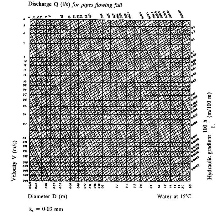
114 Hydraulics Research Station Charts To derive charts suitable for design, the Colebrook-White and Darcy-Weisbach formulas were combined to give: v ks.51ν = gdsf log D D gds f In which ν = µ ρ and is known as the kinematic viscosity and S f is the hydraulic gradient, i.e Sf = hf L. A sample chart is: 1

115 13

116 Example Problem A plastic pipe, 10 km long and 300 mm diameter, conveys water from a reservoir (water level 850 m above datum) to a water treatment plant (inlet level 700 m above datum). Assuming the reservoir remains full, estimate the discharge using the following methods: 1. the Colebrook-White formula;. the Moody diagram; 3. the HRS charts. 6 Take the kinematic viscosity to be m /s. Solution 1. Using the combined Colebrook-White and Darcy-Weisbach formula: v ks.51ν = gdsf log D D gds f We have the following input variables: 1. D = 0.3 m ;. from the table for effective roughness, k = 0.03 mm ; s 3. the hydraulic gradient is: S f = = v 6 ( ) = g( 0.3)( 0.015) log g =.514 m/s ( )( ) 14

117 Hence the discharge is: π 0.3 Q= Av =.514 = m 4 3. To use the Moody chart proceed as: 1. calculate k D; s. assume a value for v ; 3. calculate Re; 4. estimate λ from the Moody chart; 5. calculate h ; f 6. compare h with the available head, H; f 7. if hf H then repeat from step. This is obviously tedious and is the reason the HRS charts were produced. The steps are: 1. ks D 3 = = ;. We ll take v to be close to the known result from part 1 of the question to expedite the solution: 3. The Reynolds number: v =.5 m/s ; ρvl Dv Re = = for a pipe µ ν = = Referring to the Moody chart, we see that the flow is in the turbulent region. Follow the ks 6 D curve until it intersects the Re value to get: λ

118 16

119 5. The Darcy-Wesibach equation then gives: h f λlv = gd 3 ( )( ) g ( 0.3) = = m 6. The available head is H = = m so the result is quite close but this is because we assumed almost the correct answer at the start. Having confirmed the velocity using the Moody chart approach, the discharge is evaluated as before. 3. Using the HRS chart, the solution of the combined Colebrook-White and Darcy-Weisbach formula lies at the intersection of the hydraulic gradient line (sloping downwards, left to right) with the diameter (vertical) and reading off the discharge (line sloping downwards left to right): The inputs are: o S = and so 100S = 1.5 ; f f o D = 300 mm. Hence, as can be seen from the attached, we get: Q = 180 l/s = m /s Which is very similar to the exact result calculated previously. 17

120 18

121 Problems Pipe Flows 1. Determine the head loss per kilometre of a 100 mm diameter horizontal pipeline that transports oil of specific density 0.95 and viscosity Ns/m at a rate of 10 l/s. Determine also the shear stress at the pipe wall. (Ans. 9. m/km, 6.6 N/m ). A discharge of 400 l/s is to be conveyed from a reservoir at 1050 m AOD to a treatment plant at 1000 m AOD. The length of the pipeline is 5 km. Estimate the required diameter of the pipe taking k = 0.03 mm. s (Ans. 450 mm) 3. The known outflow from a distribution system is 30 l/s. The pipe diameter is 150 mm, it is 500 m long and has effective roughness of 0.03 mm. Find the head loss in the pipe using: a. the Moody formula; b. the Barr formula; c. check these value against the Colebrook-White formula. (Ans , 8.94 m) 4. A plunger of 0.08m diameter and length 0.13m has four small holes of diameter 5/1600 m drilled through in the direction of its length. The plunger is a close fit inside a cylinder, containing oil, such that no oil is assumed to pass between the plunger and the cylinder. If the plunger is subjected to a vertical downward force of 45N (including its own weight) and it is assumed that the upward flow through the four small holes is laminar, determine the speed of the fall of the plunger. The coefficient of viscosity of the oil is 0. kg/ms. (Ans m/s) 19

122 5.5 Pipe Design Local Head Losses In practice pipes have fittings such as bends, junctions, valves etc. Such features incur additional losses, termed local losses. Once again the approach to these losses is empirical, and it is found that the following is reasonably accurate: h L = k L v g In which h is the local head loss and k is a constant for a particular fitting. L L Typical values are: Fitting Local Head Loss Coefficient, k L Theoretical/Experimental Design Practice Bellmouth entrance Bellmouth exit 90 bend 90 tees: - in-line flow - branch to line - gate valve (open)

123 Sudden Enlargement Sudden enlargements (such as a pipe exiting to a tank) can be looked at theoretically: From points 1 to the velocity decreases and so the pressure increases. At 1 turbulent eddies are formed. We will assume that the pressure at 1 is the same as the pressure at 1. Apply the momentum equation between 1 and : ( ) p A p A = ρq v v Using continuity, Q= Av and so: p p v 1 = ρg g ( v v ) 1 Now apply the energy equation from 1 to : p v p v = + + h ρg g ρg g L 131

124 And so h L v v p p = g ρg 1 1 p p 1 Substituting for ρg from above: v v v 1 h = v v L g g ( ) 1 Multiplying out and rearranging: h L = ( v v ) 1 g Using continuity again, v v ( A A ) = and so: 1 1 h L A 1 v v 1 1 A = g A = 1 A v 1 1 g Therefore in the case of sudden contraction, the local head loss is given by: k L = 1 A 1 A 13

125 Sudden Contraction We use the same approach as for sudden enlargement but need to incorporate the experimental information that the area of flow at point 1 is roughly 60% of that at point. Hence: A 0.6A 1' h L 0.6A = 1 A v = 0.44 g ( v 0.6) g And so: k = L

126 Example Pipe flow incorporating local head losses Problem For the previous example of the 10 km pipe, allow for the local head losses caused by the following items: 0 90 bends; gate valves; 1 bellmouth entry; 1 bellmouth exit. Solution The available static head of 150 m is dissipated by the friction and local losses: H = h + h f L Using the table of loss coefficients, we have: h L v = ( 0 0.5) + ( 0.5) g v = 11.1 g To use the Colebrook-White formula (modified by Darcy s equation) we need to iterate as follows: 1. Assume hf. calculate v and thus h ; L H (i.e. ignore the local losses for now); 3. calculate h + h and compare to H; f L 4. If H h + h then set h = H h and repeat from. f L f L 134

127 From the last example, we will take v =.514 m/s. Thus: h L.514 = 11.1 = 3.58 m g Adjust h : f h = = m f Hence: S = = f Substitute into the Colebrook-White equation: v 6 ( ) = g( 0.3)( ) log g =.386 m/s ( )( ) Recalculate h : L h L.386 = 11.1 = 3. m g Check against H: h f + h = = m L This is sufficiently accurate and gives Q = m /s. Note that ignoring the local losses gives Q = m /s, as previous. 135

128 Partially Full Pipes Surface water and sewage pipes are designed to flow full, but not under pressure. Water mains are designed to flow full and under pressure. When a pipe is not under pressure, the water surface will be parallel to the pipe invert (the bottom of the pipe). In this case the hydraulic gradient will equal the pipe gradient, S : 0 S 0 = h f L In these non-pressurized pipes, they often do not run full and so an estimate of the velocity and discharge is required for the partially full case. This enables checking of the self-cleansing velocity (that required to keep suspended solids in motion to avoid blocking the pipe). Depending on the proportional depth of flow, the velocity and discharge will vary as shown in the following chart: 136

129 This chart uses the subscripts: p for proportion; d for partially full, and; D for full. Note that it is possible to have a higher velocity and flow when the pipe is not full due to reduced friction, but this is usually ignored in design. 137

130 Example Problem A sewerage pipe is to be laid at a gradient of 1 in 300. The design maximum discharge is 75 l/s and the design minimum flow is 10 l/s. Determine the required pipe diameter to carry the maximum discharge and maintain a self-cleansing velocity of 0.75 m/s at the minimum discharge. Solution (Note: a sewerage pipe will normally be concrete but we ll assume it s plastic here so we can use the chart for k = 0.03 mm ) s Q = 75 l/s 100hf 100 = = L 300 Using the HRS chart for k = 0.03 mm, we get: s D = 300 mm v = 1.06 m/s Check the velocity for the minimum flow of 10 l/s: 10 Q = = p 75 Hence from the proportional flow and discharge graph: d 0.5 and v 0.7 p D = = 138

131 Thus: v = = 0.76 m/s d This is greater then the minimum cleaning velocity required of 0.75 m/s and hence the 300 mm pipe is satisfactory. The lookups are: 139