2.152 Course Notes Contraction Analysis MIT, 2005

Transcription

1 2.152 Course Notes Contraction Analysis MIT, 2005 Jean-Jacques Slotine

2 Contraction Theory ẋ = f(x, t) If Θ(x, t) such that, uniformly x, t 0, F = ( Θ + Θ f x )Θ 1 < 0 Θ(x, t) T Θ(x, t) > 0 then all solutions converge exponentially to a single trajectory, independently of the initial conditions. Proof: Consider virtual displacements, δx = x(t,x o) x o δz = Θδx 1 2 dx o d dt δz 2 λ F δz 2 and path integration at fixed time.

3 Observer Lorenz attractor ẋ = σ (y x) ẏ = ρ x y x z ż = β z + x y Observer { ŷ = ρ x ŷ x ẑ ẑ = β ẑ + x ŷ J = [ 1 x x β ] < 0

4 One-Way Coupling { ẋ 1 = f(x 1, t) ẋ 2 = f(x 2, t) + u(x 1 ) u(x 2 ) If f u is contracting in an input-independent metric, then x 2 x 1 exponentially regardless of initial conditions. Extends to networks with chain or tree structure.

5 Combinations of Contracting Systems Parallel d dt δz = i α i (t) d dt δz i with α i (t) > 0, same metric Hierarchies ( ) d δz1 dt δz 2 = ( ) ( ) F1 0 δz1 F 2 δz 2 G 2 with G 2 bounded Feedback ( ) d δz1 dt δz 2 = ( ) ( ) F1 G 1 δz1 F 2 δz 2 G 2 with λ(f 1 ) λ(f 2 ) > 1 4 min K>0 σ2 (KG 1 + G T 2 ) uniformly

6 Translation and Scaling in Space and Time Multiresolutions Contracting mother system ẋ = f(x, t), constant metric. Then ẋ = f(a i (t)x b i (t), t) is contracting in the same metric, for any b i (t) and any a i (t) > 0 uniformly. So is ẋ = i α i (t) f(a i (t)x b i (t), t) for any uniformly positive α i (t). May in turn obtain α i (t) from hierarchy. So is ɛ(t) ẋ = i α i (t) f(a i (t)x b i (t), β i (t)) with ɛ(t) > 0, β i (t) 0.

7 Smooth nonlinear maps y = g(x 1,..., x n,t) where the x i are states of contracting systems (of possibly different metrics). Then δy 0 exponentially as long as all y x i are bounded. Similarly, given a contracting system of state x, boundedness of all J (i) up to order j implies exponential convergence to zero of all δx (i) up to order j + 1. The nonlinear maps may depend accordingly on time-derivatives of the x i. Any combination of all of the above

8 Parallel Combinations Control Primitives Dynamics f and primitives φ i all contracting in the same Θ(x) ẋ = f(x, t) + i α i (t) φ i (x, t) α i (t) > 0 More generally ẋ = f(x, t) + B(x, t) u Assume control primitives u = p i (x, t) make the closed-loop system contracting in common metric, i. Then any convex combination u = α i (t) p i (x, t) α i (t) 0 α i (t) = 1 i i yields a contracting dynamics in the same metric.

9 Hierarchies Composite Variables ṡ = φ(s, t) contracting by choice of control law x + λ x = s contracting by definition of s Qualitative dynamics. For instance, react faster to larger errors x x+(λ 1 +λ 2 x ) x = s x = (λ 1 +2λ 2 x ) More generally x (n) = f(x, ẋ,..., x (n 1), u, t) Target contracting system x (n) = g(x, ẋ,..., x (n 1), t) Choosing s = x (n 1) x (n 1) r d dt x(n 1) r = k s + g yields g = ṡ + k s x (n)

10 Hierarchies Motor Primitives (again) ẋ = f(x, t) + i α i (t) φ i (x, t) The α i (t) could be outputs of contracting systems higher up Periodic α i (t) lead to periodic x

11 Adaptive Combinations z = f(z, t) f(z d, t) W(z, t)ã z(t) = z(t) z d (t) â = PW T (z, t) z ã(t) = â(t) a V = d dt ( zt z + ã T P 1 ã ) = 2 z T 1 o f z (z d + λ z)dλ z Local adaptation loops: Overall sytem is nominal contracting network, driven by terms W(z, t)ã 0 Exploit physics W c (z, t)a c W(z, t)a = W c (z, t)a c + W o (z, t)a o is contracting in the same metric as f Use W c (z d, t) in place of W c (z, t) in the adaptation V = 2 z T 1 o f c z (z d + λ z)dλ z f c = f + W c a c

12 Partial Contraction Consider a nonlinear system in the form ẋ = f(x, x, t) and assume that the auxiliary system ẏ = f(y, x, t) is contracting. If a particular solution of the auxiliary system verifies a smooth specific property, then all trajectories of the original system verify this property exponentially. Proof: Another particular solution of the auxiliary system is y(t) = x(t), t 0.

13 Typically, contraction analysis not based on error signal. Rather, show closed-loop contraction, x d (t) particular solution (control) observer contraction, x(t) particular solution (estimation) More generally partial contraction, virtual contracting system such that x(t) and x d (t) are particular solutions (controller) ˆx(t) and x(t) are particular solutions (observer) Other forms of synchronization

14 Two-Way Coupling If the dynamics equations verify ẋ 1 h(x 1, t) = ẋ 2 h(x 2, t) with, in an input-independent metric, h(x, t) contracting then x 1 and x 2 converge exponentially regardless of initial conditions.

15 Proof: Define ẋ 1 h(x 1, t) = ẋ 2 h(x 2, t) = g(x 1, x 2, t) Construct an auxiliary system ẏ = h(y, t) + g(x 1, x 2, t) Two particular solutions y = x 1 (t) y = x 2 (t)

16 Example: Van der Pol oscillators { ẍ 1 + α(x 2 1 1)ẋ 1 + ω 2 x 1 = ακ 1 (ẋ 2 ẋ 1 ) ẍ 2 + α(x 2 2 1)ẋ 2 + ω 2 x 2 = ακ 2 (ẋ 1 ẋ 2 ) ẍ 1 +α(x κ 1 + κ 2 1)ẋ 1 +ω 2 x 1 = ẍ 2 +α(x κ 1 + κ 2 1)ẋ 2 +ω 2 x 2 Synchronize if κ 1 + κ 2 > 1

17 Feedback-induced oscillations Diffusion-driven instability Alan Turing, 1952 Stephen Smale, 1976 { ẍ 1 + α(x κ 1)ẋ 1 + ω 2 x 1 = ακ(ẋ 2 ẋ 1 ) ẍ 2 + α(x κ 1)ẋ 2 + ω 2 x 2 = ακ(ẋ 1 ẋ 2 ) can be written { ẍ 1 + α(x 2 1 1)ẋ 1 + ω 2 x 1 = ακ(ẋ 2 + ẋ 1 ) ẍ 2 + α(x 2 2 1)ẋ 2 + ω 2 x 2 = ακ(ẋ 1 + ẋ 2 ) so that x 2 and x 1 synchronize, for κ > 1 2.

18 { Feedback-induced oscillations ẍ 1 + α(x κ 1)ẋ 1 + ω 2 x 1 = ακ(ẋ 2 ẋ 1 ) ẍ 2 + α(x κ 1)ẋ 2 + ω 2 x 2 = ακ(ẋ 1 ẋ 2 ) Anti-synchronize if κ > 1 2

19 FitzHugh-Nagumo (1963) A classical model of spiking neurons, Hodgkin-Huxley { v = c(v + w 1 3 v3 + I) ẇ = 1 (v a + bw) c simplification of Defining Θ = [ c ] leads to generalized Jacobian F = [ c(1 v2 ) 1 1 b c ] Use coupling in v

20 Izhikevich (2004) A richer simplification of Hodgkin-Huxley { v = 0.04v 2 + 5v u + I u = a (b v u) with explicit after-spike resetting If v +30mV, then { v c u u + d Different qualitative responses based on parameter values

21

22 Analysis { v = 0.04v 2 + 5v u + I u = a (b v u) If v +30mV, then { v c u u + d Defining Θ = [ ] ab leads to generalized Jacobians F = [ ] 0.08v + 5 ab ab a F = [ ] Use coupling in v

23 Generalized Networks Consider a network of n identical systems ẋ i = f(x i, t) j N i K ji (x i x j ) Construct an auxiliary system ẏ i = f(y i, t) j N i K ji (y i y j ) K 0 Synchronization condition n y j + K 0 j=1 n x j (t) j=1 λ m+1 (L) > max i λ max (J is ) uniformly λ m+1 is first nonzero eigenvalue of coupling matrix L. That is, K 0 > 0, and K ij = K ji > 0, i, j N the network is connected λ max (J is ) is bounded and couplings are strong enough

24 Switching Networks Models of schooling fish, flocking birds, cooperating vehicles δz T δz decreases exponentially although derivative may be discontinous

25 Toy version of the proof Continuous Vicsek ẋ i = K (x i x j ) j N i (t) Auxiliary system ẏ i = K (y i y j ) K j N i (t) n (y j x j ) j=1 is contracting for K > 0 since v T J v = v j v i 2 K active links n v i 2 K i=1

26 Nonlinear couplings ẋ i = f(x i, t) + j N i u ji ( x j x i, x, t ) u ji (0, x, t) = 0 Conditions now apply to K ji = u ji ( x j x i, x, t ) (x j x i ). Such systems can be written, without loss of generality, as ẋ i = f(x i, t) + j N i K ji (x, t ) (x j x i ) Conditions apply directly to K = K(x, t ), as seen from ẏ i = f(y i, t) j N i K ji (x, t ) (y i y j ) K 0 n y j + K 0 j=1 n x j (t) j=1 For instance u ji = ( C ji (t) + L ji (t) x j x i ) (x j x i )

27 Positive semi-definite couplings K ijs = [ K ijs ] J is = [ ] J11s J 12 J T 12 J 22s i Sufficient condition for synchronization for large enough K ijs i, J 22s < 0 and λ max (J 11s ), σ max (J 12 ) bounded

28 Improve Synchronization Process Increasing the coupling gain for a link Adding an extra link..... K K..... K K.....

29 Graph Laplacian L = T K T = diag( j k ij) For an undirected graph, L is symmetric positive definite Graph diameter D, maximum distance (number of links) Mean distance ρ Standard results on D and ρ translate into sufficient conditions for synchronization where D < 4 nα or ρ < α = max i λ max (J is ) λ min (K) 2 α(n 1) + n 2 2(n 1)

30 Networks with Different Structures With n one-way ring structure λ min (K) O(n 2 ) + star structure λ min (K) O(1) all-to-all structure λ min (K) O( 1 n ) 0 Specifically, λ min (K) ring 4 λ min (K) open chain

31 Leader Following ẋ 0 = f(x 0, t) = f(x i, t) + ẋ i j N i (t) Global convergence to x 0 (γ i (t) = 0, 1 K ji (x j x i ) + γ i K 0i (x 0 x i ) i γ i(t) 1 t ) Different leaders x j 0 of arbitrary dynamics can define different group primitives which can be combined. Contraction of the followers dynamics (i = 1,..., n) ẋ i = f(x i, t) + j N i K ji (x j x i ) + j α j (t) γ j i K j 0i (x j 0 x i ) is preserved if α j (t) 1 t 0 j For subsystems with different dynamics, can combine MITwith knowledge leaders through local adaptation mechanisms.

32 Fast Inhibition ẋ i = f(x i, t) + j N i K ji (x j x i ) i = 1,..., n A single inhibitory link between two arbitrary elements has the ability to turn off the entire network. ẋ a = f(x a, t) + K ja (x j x a ) + K ( x b x a ) j N a ẋ b = f(x b, t) + K jb (x j x b ) + K ( x a x b ) j N b

33 Fast Inhibition t

34 Concurrent Synchronization Under simple conditions on the coupling strengths, the group globally exponentially synchronizes, thus providing synchronized inputs to the outer elements. So does the group. Regardless of the dynamics, connections, or inputs of the other systems. "As stable" as global exponential convergence to an equilibrium. But now to a possibly very complex coordinated behavior. The invariance itself (but not the convergence) is closely related to the notion of input-symmetry. Evolution-friendly.

35 Global exponential concurrent synchronization = Contraction to a flow-invariant linear subspace Simple conditions based on Jacobians Combination properties

36 Contraction to a Linear Subspace Theorem Consider a linear subspace M invariant for ẋ = f(x, t), let V be the orthornormal projection on M. If V ( f x) V < 0 uniformly, then all solutions converge exponentially to M. More generally, with metric Θ(x, t) Θ(x, t) on M, if ( F = Θ + ΘV f ) x V Θ 1 < 0 uniformly Proof With V V + U U = I and z = Vx, ż = Vf(V z + U Ux, t) The auxiliary contracting system ẏ = Vf(V y + U Ux, t) has y(t) = z(t) and y(t) = 0 as particular solutions.

37 For instance, for a system of the form ẋ {} = f {} (x {} ) Lx {} global exponential sync to linear invariant subspace M if [ ] λ min (VL s V f{} (x {}, t) ) > sup λ max x {},t x {} s Note percolation effect M A M B M A M B λ min (V A J s V A) λ min (V B J s V B) For identical systems subsystems and diffusion couplings [ ] f(x, t) λ min (VL s V ) > sup λ max x,t x as before, and simple extensions. s

38 Balanced diffusive networks A balanced network is a directed diffusive network which verifies for each node i j i K ij = j i K ji Because of this property, the symmetric part of its Laplacian matrix is itself the Laplacian matrix of a well-defined undirected graph. Thus, the positive definiteness of VLV is equivalent to the connectedness of the underlying undirected graph. For general networks, compute directly whether VL s V > 0.

39 Generalized diffusive connections { ẋ1 = f 1 (x 1, t) + ka (Bx 2 Ax 1 ) ẋ 2 = f 2 (x 2, t) + kb (Ax 1 Bx 2 ) where x 1 and x 2 can be of different dimensions, and A and B are constant matrices of appropriate dimensions. ( f1 ) ( ) x A J = 1 A A f 2 kl, where L = B x 2 B A B B L = L T 0 since ( ( ) ) x1 x 1 x 2 L = Ax x 1 Bx Assume that the subspace M : Ax 1 Bx 2 = 0 is flowinvariant. Using the projection V on M (so VLV > 0), for upper bounded individual Jacobians, large enough k ensures exponential convergence to M. By recursion for larger systems.

40 Excitatory-only networks { ẋ1 = f(x 1, t) + kx 2 ẋ 2 = f(x 2, t) + kx 1 J = ( f(x1,t) x 1 0 f(x 0 2,t) x 2 ) + k ( ) span{(1, 1)} is flow-invariant, with V = 1 2 (1 1) The projected Jacobian is 1 2 ( f(x 1,t) x 1 + f(x 2,t) x 2 ) k. Exponential synchronization for k > sup x,t f x. In the case of diffusive connections, once the elements are synchronized, the coupling terms disappear, so that each individual element exhibits its natural, uncoupled behaviour. This is not the case with excitatory-only connections.

41 COMBINATIONS OF CONCURRENTLY SYNCHRONIZING GROUPS Under mild conditions, global convergence to a concurrently synchronized regime is preserved under basic system combinations such as parallel, negative feedback, and hierarchies. As a result, stable concurrently synchronized aggregates of arbitrary size can be constructed. Reflects combination properties of contracting systems.

42 Input-symmetry preservation assumption Two independent groups G i of dynamical elements, each with a flow-invariant subspace M i, with V i (J i ) s V i < 0. Connect the elements of G 1 to the elements of G 2 while preserving input-symmetry for each group. Then, M 1 M 2 remains a flow-invariant subspace of the new global space. The projection on (M 1 M 2 ) is V = ( ) V V 2 where V i has been rescaled into V i for orthonormality. All results extend by recursion to combinations of arbitrary size.

43 Negative Feedback ( ) J1 kj J = 12 J 12 J 2 Metric Θ(x, t) Θ(x, t) = k > 0 ( I 0 0 ki ) on (M 1 M 2 ) Generalized projected Jacobian ( V Θ(VJV )Θ 1 = 1 J 1 V 1 k 1 V 1( kj 12)V 2 kv 2 J 12 V 1 V 2J 2 V 2 ) < 0

44 Hierarchies J = ( ) J1 0 J 12 J 2 Metric Θ(x, t) Θ(x, t) = ( I 0 0 ɛ 2 I ) on (M 1 M 2 ) Generalized projected Jacobian ( V Θ(VJV )Θ 1 = 1 J 1 V 1 0 ɛv 2J 12 V 1 V 2J 2 V 2 for bounded V 2J 12 V 1. ) < 0

45 Parallel V [ i α i(t)(j i ) s ] V = i α i(t) [V (J i ) s V ] Note superposition of different dynamics within one group. For instance, assume that for a given system ẋ = f(x, t), several types of additive couplings L i (x, t) lead stably to the same invariant set, but to different synchronized behaviors. Then any convex combination ( α i (t) 0, α i i(t) = 1 ) of the couplings will lead stably to the same invariant set. Indeed, f(x, t) i α i (t) L i (x, t) = i α i (t) [ f(x, t) L i (x, t) ] < 0 The L i (x, t) can be viewed as synchronization primitives to shape the final behavior of the combination.

46 Building concurrent synchronization one system at a time Connect single dynamics G 1 to all other elements G 2. Input-symmetry is preserved for each aspiring sync subgroup of G 2 if 1 2 connections are identical for each element. Modifying 2 1 connections does not alter input-symmetry. (M 1 M 2 ) = M 2, so concurrent synchronization and convergence rate of the combined system only depend on the parameters and states of G 2. For diffusion couplings, the projected Jacobian is V 2 ( J ind 2 K 1 2 L int ) V 2 so increase either K 1 2 or L int.

47 EXAMPLE: COINCIDENCE DETECTION, SEGMENTATION Global excitatory neuron o O... O O O FN neurons I 1 I 2 I n 1 I n

48

49 EXAMPLE: SYMMETRY DETECTION

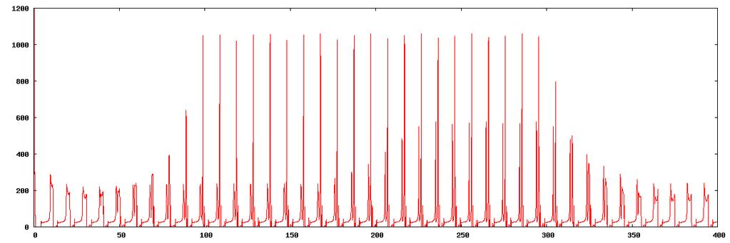
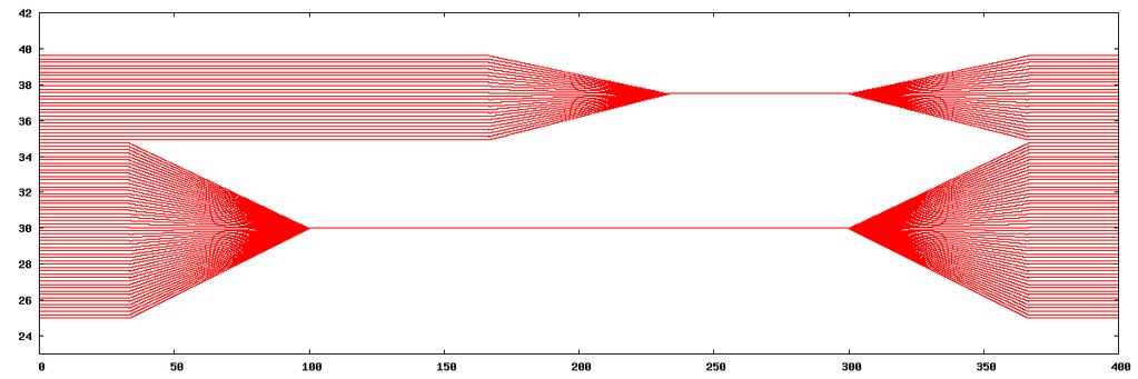
50 56 60 symmetric image 21 FN pairs on first layer, sum 8 8 inputs. At t = T/2, the window is exactly at the center of the image. v2 v1 on top layer

51 Example: Locomotion Central Pattern Generators modelled as coupled nonlinear oscillators delivering phase-locked signals. Coupled Andronov-Hopf oscillators (constant ρ, θ limit cycle) ẋ 1 = f(x 1 ) + k(rx 2 x 1 ) ẋ 2 = f(x 2 ) + k(rx 3 x 2 ) f = ( ) x y x3 xy 2 x + y y 3 yx 2 ẋ 3 = f(x 3 ) + k(rx 1 x 3 ) ( 1 R = The linear subspace M = {(R 2 (x), R(x), x) : x R 2 } is flow-invariant, and is also a subset of Null(L s ), where ) = 2π 3 rotation ẋ {} = f {} (x {} ) k Lx {} MIT The characteristic polynomial of L s is X 2 (X 3/2 )

52 The characteristic polynomial of L s is X 2 (X 3/2 ) 4. Since M is 2-dimensional, it is exactly the nullspace of L s. This implies in turn that M is the eigenspace corresponding to the eigenvalue 3/2. The eigenvalues of J s (x, y) are 1 (x 2 +y 2 ) and 1 3(x 2 +y 2 ), which are upper-bounded by 1. Thus, for k > 2/3, global exponential convergence to a ± 2π -phase-locked state. 3 Can be easily generalized to larger systems, gait primitives.

53 Extensions Not symmetric ẋ 1 = f(x 1 ) + k 1 (R 1 x 2 x 1 ) ẋ 2 = f(x 2 ) + k 2 (R 2 x 3 x 2 ) ẋ 3 = f(x 3 ) + k 3 (R 3 x 1 x 3 ) with arbitrary phase-locking R 1 R 2 R 3 = I 2. Not diffusive ẋ 1 = f(x 1 ) + krx 2 ẋ 2 = f(x 2 ) + krx 3 ẋ 3 = f(x 3 ) + krx 1 The limit cycle s radius varies with k. Larger systems, gait primitives.