Stability. Coefficients may change over time. Evolution of the economy Policy changes
|
|
|
- Lesley Gilbert
- 6 years ago
- Views:
Transcription
1 Sabiliy Coefficiens may change over ime Evoluion of he economy Policy changes
2 Time Varying Parameers y = α + x β + Coefficiens depend on he ime period If he coefficiens vary randomly and are unpredicable, hen hey canno be esimaed As here would be only one observaion for each se of coefficiens We canno esimae coefficiens from jus one observaion! e
3 Smoohly Time Varying Parameers y = α + x β + If he coefficiens change gradually over ime, hen he coefficiens are similar in adjacen ime periods. We could ry o esimae he coefficiens for ime period by esimaing he regression using observaions [ w/2,, + w/2] where w is called he window widh. w is he number of observaions used for local esimaion e
4 Rolling Esimaion This is called rolling esimaion For a given window widh w, you roll hrough he sample, using w observaions for esimaion. You advance one observaion a a ime and repea Then you can plo he esimaed coefficiens agains ime
5 Wha o expec Rolling esimaes will be a combinaion of rue coefficiens and sampling error The sampling error can be large Flucuaions in he esimaes can be jus error If he rue coefficiens are rending Expec he esimaed coefficiens o display rend plus noise If he rue coefficiens are consan Expec he esimaed coefficiens o display random flucuaion and noise

6 Example: GDP Growh
7 STATA rolling command STATA has a command for rolling esimaion:.rolling, window(100) clear: regress gdp L(1/3).gdp In his command: window(100) ses he window widh w=100 The number of observaions for esimaion will be 100 clear Clears ou he daa in memory The daa will be replaced by he rolling esimaes I is necessary
8 rolling command.rolling, window(100) clear: regress gdp L(1/3).gdp The par afer he : regress gdp L(1/3).gdp This is he command ha STATA will implemen using he rolling mehod An AR(3) will be fi using 100 observaions, rolling hrough he sample
9 Example GDP, quarerly, 1947Q1 hrough 2009Q4 251 observaions Using w=100 The firs esimaion window is 1947Q2 1972Q1 The second is 1947Q3 1972Q2 There are 152 esimaion windows The final is 1985Q1 2009Q4

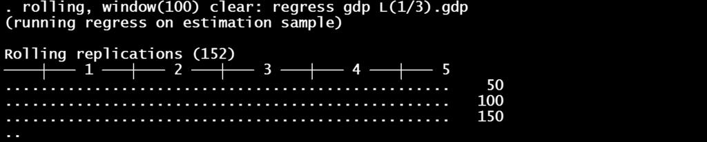
10 STATA Execuion:
11 Afer Rolling Execuion The original daa have been cleared from memory STATA shows new variables sar end _sa_1 _sa_2 _sa_3 _b_cons sar and end are saring/ending daes for each window sar runs from 1947Q2 o 1985Q1 end runs from o 1972Q1 2009Q4 The ohers are he rolling esimaes, AR and inercep
12 Time rese As he original daa have been cleared, so has your ime index. So he sline command does no work unil you rese he ime You can se he ime o be sar or end.sse sar.sse end Or, more eleganly, you can se he ime o be he midpoin of he window.gen =round((sar+end)/2).forma %q.sse This ime index runs from 1959Q4 hrough 1997Q3

13 Example Time rese example
14 Plo Rolling Coefficiens Now you can plo he esimaed coefficiens agains ime You can use separae or join plos.sline _b_cons.sline _sa_1 _sa_2 _sa_3

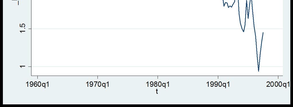
15 Rolling Inercep
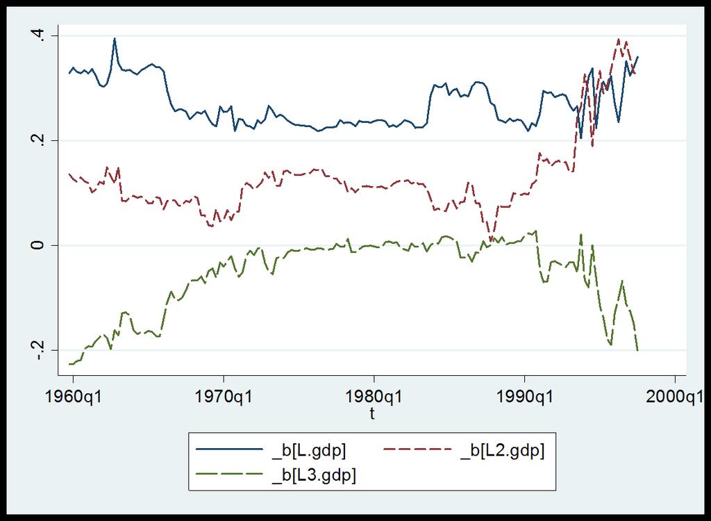
16 Rolling AR coefficiens
 coef is 0 mos of he period, bu is negaive from 1960 1973 and afer 1995 All of he graphs go a bi crazy over 1990")
17 Analysis The esimaed inercep is decreasing gradually The AR(1) coef is quie sable The AR(2) coef sars increasing around 1990 The AR(3) coef is 0 mos of he period, bu is negaive from and afer 1995 All of he graphs go a bi crazy over
18 Sequenial (Recursive) Esimaion As an alernaive o rolling esimaion, sequenial or recursive esimaion uses all he daa up o he window widh Firs window: [1,w] Second window: [1,w+1] Final window: [1,T] Wih sequenial esimaion, window is he lengh of he firs esimaion window
19 Recursive Esimaion STATA command is similar, bu adds recursive afer comma.rolling, recursive window(100) clear: regress gdp L(1/3).gdp STATA clears daa se, replaces wih sar, end, and recursive coefficien esimaes _b_cons, _sa_1, ec. Use end for ime variable.sse end This ses he ime index o he end period used for esimaion
20 Recursive Inercep

21 Recursive AR coefficiens
 and AR(2) coefs are very sable The recursive AR(3) coef increases, and hen becomes sable afer")
22 Analysis The recursive inercep flucuaes, bu decreases Drops around 1984, and 1990 The recursive AR(1) and AR(2) coefs are very sable The recursive AR(3) coef increases, and hen becomes sable afer 1984.
23 Summary Use rolling and recursive esimaion o invesigae sabiliy of esimaed coefficiens Look for paerns and evidence of change Try o idenify poenial breakdaes In GDP example, possible daes: 1970, 1984, 1990
24 Tesing for Breaks Did he coefficiens change a some breakdae *? We can es if he coefficiens before and afer * are he same, or if hey changed Simple o implemen as an F es using dummy variables Known as a Chow es
 Proposed he Chow Tes for srucural change in a famous")
25 Gregory Chow Professor Gregory Chow of Princeon Universiy (emerius) Proposed he Chow Tes for srucural change in a famous paper in 1960
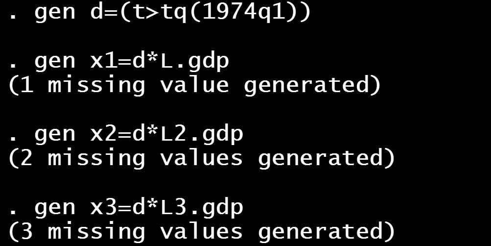
26 Dummy Variable For a given breakdae * Define a dummy variable d d=1 if >* Include d and ineracions d*x o es for changes
27 Model wih Breaks Original Model y = α + x β + e Model wih break y = α + x β + δd + γd x + Inerpreing he coefficiens δ=change in inercep γ=change in slope e
28 Chow Tes y = α + x β + δd + γd x + e The model has consan parameers if δ=γ=0 Hypohesis es: H 0 : δ=0 and γ=0 Implemen as an F es afer esimaion If prob>.05, you do no rejec he hypohesis of sable coefficiens

29 Example: GDP
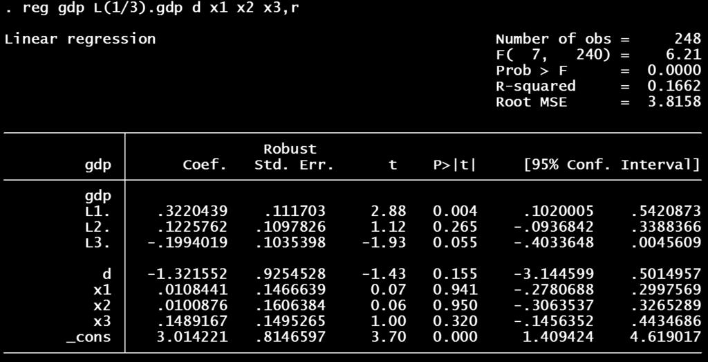
30

31 Chow es The p value is larger han 0.05 I is no significan We do no rejec hypohesis of consan coefficiens
32 Fishing for a Breakdae An imporan rouble wih he Chow es is ha i assumes ha he breakdae is known before looking a he daa Bu we seleced he breakdae by examining rolling and recursive esimaes This means ha are oo likely o find misleading evidence of non consan coefficiens
33 Fishing We could consider picking muliple possible breakdaes *=[ 1, 2,, M ] For each breakdae *, we could esimae he regression and compue he Chow saisic F(*) Fishing for a breakdae is similar o searching for a big (significan) Chow saisic.
34 The Quand Likelihod Raio (QLR) Saisic (also called he sup Wald saisic) The QLR saisic = he maximal Chow saisics Le F(τ) = he Chow es saisic esing he hypohesis of no break a dae τ. The QLR es saisic is he maximum of all he Chow F- saisics, over a range of τ, τ 0 τ τ 1 : QLR = max[f(τ 0 ), F(τ 0 +1),, F(τ 1 1), F(τ 1 )] A convenional choice for τ 0 and τ 1 are he inner 70% of he sample (exclude he firs and las 15%. 34
35 Richard Quand Professor Richard Quand (1930 ) Princeon Universiy Esimaion of breakdae (Quand, 1958) QLR es (Quand, 1960)
36 QLR Criical Values QLR = max[f(τ 0 ), F(τ 0 +1),, F(τ 1 1), F(τ 1 )] Should you use he usual criical values? The large-sample null disribuion of F(τ) for a given (fixed, no esimaed) τ is F q, Bu if you ge o compue wo Chow ess and choose he bigges one, he criical value mus be larger han he criical value for a single Chow es. If you compue very many Chow es saisics for example, all daes in he cenral 70% of he sample he criical value mus be larger sill! 36
37 Ge his: in large samples, QLR has he disribuion, max a s 1 a q 2 1 Bi ( s) q i= 1 s(1 s), where {B i }, i =1,,n, are independen coninuous-ime Brownian Bridges on 0 s 1 (a Brownian Bridge is a Brownian moion deviaed from is mean), and where a =.15 (exclude firs and las 15% of he sample) Criical values are abulaed in SW Table

38 Noe ha hese criical values are larger han he F q, criical values for example, F 1, 5% criical value is
39 QLR Theory Disribuion heory for he QLR saisic Developed by Professor Donald Andrews (Yale)
40 Has he poswar U.S. Phillips Curve been sable? Consider a model of ΔInf given Unemp he empirical backwards-looking Phillips curve, esimaed over ( ): Δ Inf = ΔInf 1.37ΔInf ΔInf 3.04ΔInf 4 (.44) (.08) (.09) (.08) (.08) 2.64Unem Unem Unem Unemp 4 (.46) (.86) (.89) (.45) Has his model been sable over he full period ? 40
41 QLR ess of sabiliy of he Phillips curve. dependen variable: ΔInf regressors: inercep, ΔInf 1,, ΔInf 4, Unemp 1,, Unemp 4 es for consancy of inercep only (oher coefficiens are assumed consan): QLR = (q = 1). 10% criical value = 7.12 don rejec a 10% level es for consancy of inercep and coefficiens on Unemp,, Unemp 3 (coefficiens on ΔInf 1,, ΔInf 4 are consan): QLR = (q = 5) 1% criical value = 4.53 rejec a 1% level Break dae esimae: maximal F occurs in 1981:IV Conclude ha here is a break in he inflaion unemploymen relaion, wih esimaed dae of 1981:IV 41
42 42
43 Implemenaion I is difficul o compue QLR wihou using some programming. Bu i is well approximaed by Examining rolling and recursive esimaes for possible breaks Compuing Chow es a poenial breakdaes. Don use STATA s p value! Use Table 14.6 from SW (or earlier slide).
Estimation Uncertainty
 Esimaion Uncerainy The sample mean is an esimae of β = E(y +h ) The esimaion error is = + = T h y T b ( ) = = + = + = = = T T h T h e T y T y T b β β β Esimaion Variance Under classical condiions, where
Distribution of Estimates
 Disribuion of Esimaes From Economerics (40) Linear Regression Model Assume (y,x ) is iid and E(x e )0 Esimaion Consisency y α + βx + he esimaes approach he rue values as he sample size increases Esimaion
Wisconsin Unemployment Rate Forecast Revisited
 Wisconsin Unemploymen Rae Forecas Revisied Forecas in Lecure Wisconsin unemploymen November 06 was 4.% Forecass Poin Forecas 50% Inerval 80% Inerval Forecas Forecas December 06 4.0% (4.0%, 4.0%) (3.95%,
Distribution of Least Squares
 Disribuion of Leas Squares In classic regression, if he errors are iid normal, and independen of he regressors, hen he leas squares esimaes have an exac normal disribuion, no jus asympoic his is no rue
Comparing Means: t-tests for One Sample & Two Related Samples
 Comparing Means: -Tess for One Sample & Two Relaed Samples Using he z-tes: Assumpions -Tess for One Sample & Two Relaed Samples The z-es (of a sample mean agains a populaion mean) is based on he assumpion
Financial Econometrics Jeffrey R. Russell Midterm Winter 2009 SOLUTIONS
 Name SOLUTIONS Financial Economerics Jeffrey R. Russell Miderm Winer 009 SOLUTIONS You have 80 minues o complee he exam. Use can use a calculaor and noes. Try o fi all your work in he space provided. If
R t. C t P t. + u t. C t = αp t + βr t + v t. + β + w t
 Exercise 7 C P = α + β R P + u C = αp + βr + v (a) (b) C R = α P R + β + w (c) Assumpions abou he disurbances u, v, w : Classical assumions on he disurbance of one of he equaions, eg. on (b): E(v v s P,
ACE 564 Spring Lecture 7. Extensions of The Multiple Regression Model: Dummy Independent Variables. by Professor Scott H.
 ACE 564 Spring 2006 Lecure 7 Exensions of The Muliple Regression Model: Dumm Independen Variables b Professor Sco H. Irwin Readings: Griffihs, Hill and Judge. "Dumm Variables and Varing Coefficien Models
Vectorautoregressive Model and Cointegration Analysis. Time Series Analysis Dr. Sevtap Kestel 1
 Vecorauoregressive Model and Coinegraion Analysis Par V Time Series Analysis Dr. Sevap Kesel 1 Vecorauoregression Vecor auoregression (VAR) is an economeric model used o capure he evoluion and he inerdependencies
Licenciatura de ADE y Licenciatura conjunta Derecho y ADE. Hoja de ejercicios 2 PARTE A
 Licenciaura de ADE y Licenciaura conjuna Derecho y ADE Hoja de ejercicios PARTE A 1. Consider he following models Δy = 0.8 + ε (1 + 0.8L) Δ 1 y = ε where ε and ε are independen whie noise processes. In
Time series Decomposition method
 Time series Decomposiion mehod A ime series is described using a mulifacor model such as = f (rend, cyclical, seasonal, error) = f (T, C, S, e) Long- Iner-mediaed Seasonal Irregular erm erm effec, effec,
Econ Autocorrelation. Sanjaya DeSilva
 Econ 39 - Auocorrelaion Sanjaya DeSilva Ocober 3, 008 1 Definiion Auocorrelaion (or serial correlaion) occurs when he error erm of one observaion is correlaed wih he error erm of any oher observaion. This
GDP Advance Estimate, 2016Q4
 GDP Advance Esimae, 26Q4 Friday, Jan 27 Real gross domesic produc (GDP) increased a an annual rae of.9 percen in he fourh quarer of 26. The deceleraion in real GDP in he fourh quarer refleced a downurn
Econ107 Applied Econometrics Topic 7: Multicollinearity (Studenmund, Chapter 8)
") I. Definiions and Problems A. Perfec Mulicollineariy Econ7 Applied Economerics Topic 7: Mulicollineariy (Sudenmund, Chaper 8) Definiion: Perfec mulicollineariy exiss in a following K-variable regression
I. Definiions and Problems A. Perfec Mulicollineariy Econ7 Applied Economerics Topic 7: Mulicollineariy (Sudenmund, Chaper 8) Definiion: Perfec mulicollineariy exiss in a following K-variable regression
Wednesday, November 7 Handout: Heteroskedasticity
 Amhers College Deparmen of Economics Economics 360 Fall 202 Wednesday, November 7 Handou: Heeroskedasiciy Preview Review o Regression Model o Sandard Ordinary Leas Squares (OLS) Premises o Esimaion Procedures
Solutions: Wednesday, November 14
 Amhers College Deparmen of Economics Economics 360 Fall 2012 Soluions: Wednesday, November 14 Judicial Daa: Cross secion daa of judicial and economic saisics for he fify saes in 2000. JudExp CrimesAll
Lecture 3: Exponential Smoothing
 NATCOR: Forecasing & Predicive Analyics Lecure 3: Exponenial Smoohing John Boylan Lancaser Cenre for Forecasing Deparmen of Managemen Science Mehods and Models Forecasing Mehod A (numerical) procedure
Stationary Time Series
 3-Jul-3 Time Series Analysis Assoc. Prof. Dr. Sevap Kesel July 03 Saionary Time Series Sricly saionary process: If he oin dis. of is he same as he oin dis. of ( X,... X n) ( X h,... X nh) Weakly Saionary
Lecture 15. Dummy variables, continued
 Lecure 15. Dummy variables, coninued Seasonal effecs in ime series Consider relaion beween elecriciy consumpion Y and elecriciy price X. The daa are quarerly ime series. Firs model ln α 1 + α2 Y = ln X
Solutions to Odd Number Exercises in Chapter 6
 1 Soluions o Odd Number Exercises in 6.1 R y eˆ 1.7151 y 6.3 From eˆ ( T K) ˆ R 1 1 SST SST SST (1 R ) 55.36(1.7911) we have, ˆ 6.414 T K ( ) 6.5 y ye ye y e 1 1 Consider he erms e and xe b b x e y e b
Properties of Autocorrelated Processes Economics 30331
 Properies of Auocorrelaed Processes Economics 3033 Bill Evans Fall 05 Suppose we have ime series daa series labeled as where =,,3, T (he final period) Some examples are he dail closing price of he S&500,
ECON 482 / WH Hong Time Series Data Analysis 1. The Nature of Time Series Data. Example of time series data (inflation and unemployment rates)
") ECON 48 / WH Hong Time Series Daa Analysis. The Naure of Time Series Daa Example of ime series daa (inflaion and unemploymen raes) ECON 48 / WH Hong Time Series Daa Analysis The naure of ime series daa
ECON 48 / WH Hong Time Series Daa Analysis. The Naure of Time Series Daa Example of ime series daa (inflaion and unemploymen raes) ECON 48 / WH Hong Time Series Daa Analysis The naure of ime series daa
How to Deal with Structural Breaks in Practical Cointegration Analysis
 How o Deal wih Srucural Breaks in Pracical Coinegraion Analysis Roselyne Joyeux * School of Economic and Financial Sudies Macquarie Universiy December 00 ABSTRACT In his noe we consider he reamen of srucural
1. Diagnostic (Misspeci cation) Tests: Testing the Assumptions
 Tests: Testing the Assumptions") Business School, Brunel Universiy MSc. EC5501/5509 Modelling Financial Decisions and Markes/Inroducion o Quaniaive Mehods Prof. Menelaos Karanasos (Room SS269, el. 01895265284) Lecure Noes 6 1. Diagnosic
Business School, Brunel Universiy MSc. EC5501/5509 Modelling Financial Decisions and Markes/Inroducion o Quaniaive Mehods Prof. Menelaos Karanasos (Room SS269, el. 01895265284) Lecure Noes 6 1. Diagnosic
Bias in Conditional and Unconditional Fixed Effects Logit Estimation: a Correction * Tom Coupé
 Bias in Condiional and Uncondiional Fixed Effecs Logi Esimaion: a Correcion * Tom Coupé Economics Educaion and Research Consorium, Naional Universiy of Kyiv Mohyla Academy Address: Vul Voloska 10, 04070
Introduction D P. r = constant discount rate, g = Gordon Model (1962): constant dividend growth rate.
: constant dividend growth rate.") Inroducion Gordon Model (1962): D P = r g r = consan discoun rae, g = consan dividend growh rae. If raional expecaions of fuure discoun raes and dividend growh vary over ime, so should he D/P raio. Since
Inroducion Gordon Model (1962): D P = r g r = consan discoun rae, g = consan dividend growh rae. If raional expecaions of fuure discoun raes and dividend growh vary over ime, so should he D/P raio. Since
Regression with Time Series Data
 Regression wih Time Series Daa y = β 0 + β 1 x 1 +...+ β k x k + u Serial Correlaion and Heeroskedasiciy Time Series - Serial Correlaion and Heeroskedasiciy 1 Serially Correlaed Errors: Consequences Wih
Modeling and Forecasting Volatility Autoregressive Conditional Heteroskedasticity Models. Economic Forecasting Anthony Tay Slide 1
 Modeling and Forecasing Volailiy Auoregressive Condiional Heeroskedasiciy Models Anhony Tay Slide 1 smpl @all line(m) sii dl_sii S TII D L _ S TII 4,000. 3,000.1.0,000 -.1 1,000 -. 0 86 88 90 9 94 96 98
Math 10B: Mock Mid II. April 13, 2016
 Name: Soluions Mah 10B: Mock Mid II April 13, 016 1. ( poins) Sae, wih jusificaion, wheher he following saemens are rue or false. (a) If a 3 3 marix A saisfies A 3 A = 0, hen i canno be inverible. True.
Diebold, Chapter 7. Francis X. Diebold, Elements of Forecasting, 4th Edition (Mason, Ohio: Cengage Learning, 2006). Chapter 7. Characterizing Cycles
. Chapter 7. Characterizing Cycles") Diebold, Chaper 7 Francis X. Diebold, Elemens of Forecasing, 4h Ediion (Mason, Ohio: Cengage Learning, 006). Chaper 7. Characerizing Cycles Afer compleing his reading you should be able o: Define covariance
Diebold, Chaper 7 Francis X. Diebold, Elemens of Forecasing, 4h Ediion (Mason, Ohio: Cengage Learning, 006). Chaper 7. Characerizing Cycles Afer compleing his reading you should be able o: Define covariance
Ensamble methods: Bagging and Boosting
 Lecure 21 Ensamble mehods: Bagging and Boosing Milos Hauskrech milos@cs.pi.edu 5329 Senno Square Ensemble mehods Mixure of expers Muliple base models (classifiers, regressors), each covers a differen par
13.3 Term structure models
 13.3 Term srucure models 13.3.1 Expecaions hypohesis model - Simples "model" a) shor rae b) expecaions o ge oher prices Resul: y () = 1 h +1 δ = φ( δ)+ε +1 f () = E (y +1) (1) =δ + φ( δ) f (3) = E (y +)
Exponential Smoothing
 Exponenial moohing Inroducion A simple mehod for forecasing. Does no require long series. Enables o decompose he series ino a rend and seasonal effecs. Paricularly useful mehod when here is a need o forecas
Unit Root Time Series. Univariate random walk
 Uni Roo ime Series Univariae random walk Consider he regression y y where ~ iid N 0, he leas squares esimae of is: ˆ yy y y yy Now wha if = If y y hen le y 0 =0 so ha y j j If ~ iid N 0, hen y ~ N 0, he
Types of Exponential Smoothing Methods. Simple Exponential Smoothing. Simple Exponential Smoothing
 M Business Forecasing Mehods Exponenial moohing Mehods ecurer : Dr Iris Yeung Room No : P79 Tel No : 788 8 Types of Exponenial moohing Mehods imple Exponenial moohing Double Exponenial moohing Brown s
A Dynamic Model of Economic Fluctuations
 CHAPTER 15 A Dynamic Model of Economic Flucuaions Modified for ECON 2204 by Bob Murphy 2016 Worh Publishers, all righs reserved IN THIS CHAPTER, OU WILL LEARN: how o incorporae dynamics ino he AD-AS model
Cointegration and Implications for Forecasting
 Coinegraion and Implicaions for Forecasing Two examples (A) Y Y 1 1 1 2 (B) Y 0.3 0.9 1 1 2 Example B: Coinegraion Y and coinegraed wih coinegraing vecor [1, 0.9] because Y 0.9 0.3 is a saionary process
Outline. lse-logo. Outline. Outline. 1 Wald Test. 2 The Likelihood Ratio Test. 3 Lagrange Multiplier Tests
 Ouline Ouline Hypohesis Tes wihin he Maximum Likelihood Framework There are hree main frequenis approaches o inference wihin he Maximum Likelihood framework: he Wald es, he Likelihood Raio es and he Lagrange
Methodology. -ratios are biased and that the appropriate critical values have to be increased by an amount. that depends on the sample size.
 Mehodology. Uni Roo Tess A ime series is inegraed when i has a mean revering propery and a finie variance. I is only emporarily ou of equilibrium and is called saionary in I(0). However a ime series ha
Ensamble methods: Boosting
 Lecure 21 Ensamble mehods: Boosing Milos Hauskrech milos@cs.pi.edu 5329 Senno Square Schedule Final exam: April 18: 1:00-2:15pm, in-class Term projecs April 23 & April 25: a 1:00-2:30pm in CS seminar room
Summer Term Albert-Ludwigs-Universität Freiburg Empirische Forschung und Okonometrie. Time Series Analysis
 Summer Term 2009 Alber-Ludwigs-Universiä Freiburg Empirische Forschung und Okonomerie Time Series Analysis Classical Time Series Models Time Series Analysis Dr. Sevap Kesel 2 Componens Hourly earnings:
EXERCISES FOR SECTION 1.5
 1.5 Exisence and Uniqueness of Soluions 43 20. 1 v c 21. 1 v c 1 2 4 6 8 10 1 2 2 4 6 8 10 Graph of approximae soluion obained using Euler s mehod wih = 0.1. Graph of approximae soluion obained using Euler
ESTIMATION OF DYNAMIC PANEL DATA MODELS WHEN REGRESSION COEFFICIENTS AND INDIVIDUAL EFFECTS ARE TIME-VARYING
 Inernaional Journal of Social Science and Economic Research Volume:02 Issue:0 ESTIMATION OF DYNAMIC PANEL DATA MODELS WHEN REGRESSION COEFFICIENTS AND INDIVIDUAL EFFECTS ARE TIME-VARYING Chung-ki Min Professor
TÁMOP /2/A/KMR
 ECONOMIC STATISTICS ECONOMIC STATISTICS Sonsored by a Gran TÁMOP-4..2-08/2/A/KMR-2009-004 Course Maerial Develoed by Dearmen of Economics, Faculy of Social Sciences, Eövös Loránd Universiy Budaes (ELTE)
Simulation-Solving Dynamic Models ABE 5646 Week 2, Spring 2010
 Simulaion-Solving Dynamic Models ABE 5646 Week 2, Spring 2010 Week Descripion Reading Maerial 2 Compuer Simulaion of Dynamic Models Finie Difference, coninuous saes, discree ime Simple Mehods Euler Trapezoid
Physics 235 Chapter 2. Chapter 2 Newtonian Mechanics Single Particle
 Chaper 2 Newonian Mechanics Single Paricle In his Chaper we will review wha Newon s laws of mechanics ell us abou he moion of a single paricle. Newon s laws are only valid in suiable reference frames,
(a) Set up the least squares estimation procedure for this problem, which will consist in minimizing the sum of squared residuals. 2 t.
 Set up the least squares estimation procedure for this problem, which will consist in minimizing the sum of squared residuals. 2 t.") Insrucions: The goal of he problem se is o undersand wha you are doing raher han jus geing he correc resul. Please show your work clearly and nealy. No credi will be given o lae homework, regardless of
Insrucions: The goal of he problem se is o undersand wha you are doing raher han jus geing he correc resul. Please show your work clearly and nealy. No credi will be given o lae homework, regardless of
Dynamic Econometric Models: Y t = + 0 X t + 1 X t X t k X t-k + e t. A. Autoregressive Model:
 Dynamic Economeric Models: A. Auoregressive Model: Y = + 0 X 1 Y -1 + 2 Y -2 + k Y -k + e (Wih lagged dependen variable(s) on he RHS) B. Disribued-lag Model: Y = + 0 X + 1 X -1 + 2 X -2 + + k X -k + e
Innova Junior College H2 Mathematics JC2 Preliminary Examinations Paper 2 Solutions 0 (*)
") Soluion 3 x 4x3 x 3 x 0 4x3 x 4x3 x 4x3 x 4x3 x x 3x 3 4x3 x Innova Junior College H Mahemaics JC Preliminary Examinaions Paper Soluions 3x 3 4x 3x 0 4x 3 4x 3 0 (*) 0 0 + + + - 3 3 4 3 3 3 3 Hence x or
Soluion 3 x 4x3 x 3 x 0 4x3 x 4x3 x 4x3 x 4x3 x x 3x 3 4x3 x Innova Junior College H Mahemaics JC Preliminary Examinaions Paper Soluions 3x 3 4x 3x 0 4x 3 4x 3 0 (*) 0 0 + + + - 3 3 4 3 3 3 3 Hence x or
GMM - Generalized Method of Moments
 GMM - Generalized Mehod of Momens Conens GMM esimaion, shor inroducion 2 GMM inuiion: Maching momens 2 3 General overview of GMM esimaion. 3 3. Weighing marix...........................................
Nonstationarity-Integrated Models. Time Series Analysis Dr. Sevtap Kestel 1
 Nonsaionariy-Inegraed Models Time Series Analysis Dr. Sevap Kesel 1 Diagnosic Checking Residual Analysis: Whie noise. P-P or Q-Q plos of he residuals follow a normal disribuion, he series is called a Gaussian
Mean Reversion of Balance of Payments GEvidence from Sequential Trend Break Unit Root Tests. Abstract
 Mean Reversion of Balance of Paymens GEvidence from Sequenial Trend Brea Uni Roo Tess Mei-Yin Lin Deparmen of Economics, Shih Hsin Universiy Jue-Shyan Wang Deparmen of Public Finance, Naional Chengchi
15. Which Rule for Monetary Policy?
 15. Which Rule for Moneary Policy? John B. Taylor, May 22, 2013 Sared Course wih a Big Policy Issue: Compeing Moneary Policies Fed Vice Chair Yellen described hese in her April 2012 paper, as discussed
STAD57 Time Series Analysis. Lecture 5
 STAD57 Time Series Analysis Lecure 5 1 Exploraory Daa Analysis Check if given TS is saionary: µ is consan σ 2 is consan γ(s,) is funcion of h= s If no, ry o make i saionary using some of he mehods below:
3.1 More on model selection
 3. More on Model selecion 3. Comparing models AIC, BIC, Adjused R squared. 3. Over Fiing problem. 3.3 Sample spliing. 3. More on model selecion crieria Ofen afer model fiing you are lef wih a handful of
You must fully interpret your results. There is a relationship doesn t cut it. Use the text and, especially, the SPSS Manual for guidance.
 POLI 30D SPRING 2015 LAST ASSIGNMENT TRUMPETS PLEASE!!!!! Due Thursday, December 10 (or sooner), by 7PM hrough TurnIIn I had his all se up in my mind. You would use regression analysis o follow up on your
Dynamic Models, Autocorrelation and Forecasting
 ECON 4551 Economerics II Memorial Universiy of Newfoundland Dynamic Models, Auocorrelaion and Forecasing Adaped from Vera Tabakova s noes 9.1 Inroducion 9.2 Lags in he Error Term: Auocorrelaion 9.3 Esimaing
Lecture 5. Time series: ECM. Bernardina Algieri Department Economics, Statistics and Finance
 Lecure 5 Time series: ECM Bernardina Algieri Deparmen Economics, Saisics and Finance Conens Time Series Modelling Coinegraion Error Correcion Model Two Seps, Engle-Granger procedure Error Correcion Model
ADVANCED MATHEMATICS FOR ECONOMICS /2013 Sheet 3: Di erential equations
 ADVANCED MATHEMATICS FOR ECONOMICS - /3 Shee 3: Di erenial equaions Check ha x() =± p ln(c( + )), where C is a posiive consan, is soluion of he ODE x () = Solve he following di erenial equaions: (a) x
Vehicle Arrival Models : Headway
 Chaper 12 Vehicle Arrival Models : Headway 12.1 Inroducion Modelling arrival of vehicle a secion of road is an imporan sep in raffic flow modelling. I has imporan applicaion in raffic flow simulaion where
OBJECTIVES OF TIME SERIES ANALYSIS
 OBJECTIVES OF TIME SERIES ANALYSIS Undersanding he dynamic or imedependen srucure of he observaions of a single series (univariae analysis) Forecasing of fuure observaions Asceraining he leading, lagging
Empirical Process Theory
 Empirical Process heory 4.384 ime Series Analysis, Fall 27 Reciaion by Paul Schrimpf Supplemenary o lecures given by Anna Mikusheva Ocober 7, 28 Reciaion 7 Empirical Process heory Le x be a real-valued
Stat 601 The Design of Experiments
 Sa 601 The Design of Experimens Yuqing Xu Deparmen of Saisics Universiy of Wisconsin Madison, WI 53706, USA December 1, 2016 Yuqing Xu (UW-Madison) Sa 601 Week 12 December 1, 2016 1 / 17 Lain Squares Definiion
A Specification Test for Linear Dynamic Stochastic General Equilibrium Models
 Journal of Saisical and Economeric Mehods, vol.1, no.2, 2012, 65-70 ISSN: 2241-0384 (prin), 2241-0376 (online) Scienpress Ld, 2012 A Specificaion Tes for Linear Dynamic Sochasic General Equilibrium Models
The Effect of Nonzero Autocorrelation Coefficients on the Distributions of Durbin-Watson Test Estimator: Three Autoregressive Models
 EJ Exper Journal of Economi c s ( 4 ), 85-9 9 4 Th e Au h or. Publi sh ed by Sp rin In v esify. ISS N 3 5 9-7 7 4 Econ omics.e xp erjou rn a ls.com The Effec of Nonzero Auocorrelaion Coefficiens on he
Some Basic Information about M-S-D Systems
 Some Basic Informaion abou M-S-D Sysems 1 Inroducion We wan o give some summary of he facs concerning unforced (homogeneous) and forced (non-homogeneous) models for linear oscillaors governed by second-order,
Generalized Least Squares
 Generalized Leas Squares Augus 006 1 Modified Model Original assumpions: 1 Specificaion: y = Xβ + ε (1) Eε =0 3 EX 0 ε =0 4 Eεε 0 = σ I In his secion, we consider relaxing assumpion (4) Insead, assume
Section 7.4 Modeling Changing Amplitude and Midline
 488 Chaper 7 Secion 7.4 Modeling Changing Ampliude and Midline While sinusoidal funcions can model a variey of behaviors, i is ofen necessary o combine sinusoidal funcions wih linear and exponenial curves
Biol. 356 Lab 8. Mortality, Recruitment, and Migration Rates
 Biol. 356 Lab 8. Moraliy, Recruimen, and Migraion Raes (modified from Cox, 00, General Ecology Lab Manual, McGraw Hill) Las week we esimaed populaion size hrough several mehods. One assumpion of all hese
Chapter 2. Models, Censoring, and Likelihood for Failure-Time Data
 Chaper 2 Models, Censoring, and Likelihood for Failure-Time Daa William Q. Meeker and Luis A. Escobar Iowa Sae Universiy and Louisiana Sae Universiy Copyrigh 1998-2008 W. Q. Meeker and L. A. Escobar. Based
The equation to any straight line can be expressed in the form:
 Sring Graphs Par 1 Answers 1 TI-Nspire Invesigaion Suden min Aims Deermine a series of equaions of sraigh lines o form a paern similar o ha formed by he cables on he Jerusalem Chords Bridge. Deermine he
Fishing limits and the Logistic Equation. 1
 Fishing limis and he Logisic Equaion. 1 1. The Logisic Equaion. The logisic equaion is an equaion governing populaion growh for populaions in an environmen wih a limied amoun of resources (for insance,
Lesson 2, page 1. Outline of lesson 2
 Lesson 2, page Ouline of lesson 2 Inroduce he Auocorrelaion Coefficien Undersand and define saionariy Discuss ransformaion Discuss rend and rend removal C:\Kyrre\sudier\drgrad\Kurs\series\lecure 02 03022.doc,
Lecture 2-1 Kinematics in One Dimension Displacement, Velocity and Acceleration Everything in the world is moving. Nothing stays still.
 Lecure - Kinemaics in One Dimension Displacemen, Velociy and Acceleraion Everyhing in he world is moving. Nohing says sill. Moion occurs a all scales of he universe, saring from he moion of elecrons in
Chapter 16. Regression with Time Series Data
 Chaper 16 Regression wih Time Series Daa The analysis of ime series daa is of vial ineres o many groups, such as macroeconomiss sudying he behavior of naional and inernaional economies, finance economiss
ACE 562 Fall Lecture 5: The Simple Linear Regression Model: Sampling Properties of the Least Squares Estimators. by Professor Scott H.
 ACE 56 Fall 005 Lecure 5: he Simple Linear Regression Model: Sampling Properies of he Leas Squares Esimaors by Professor Sco H. Irwin Required Reading: Griffihs, Hill and Judge. "Inference in he Simple
Ready for euro? Empirical study of the actual monetary policy independence in Poland VECM modelling
 Macroeconomerics Handou 2 Ready for euro? Empirical sudy of he acual moneary policy independence in Poland VECM modelling 1. Inroducion This classes are based on: Łukasz Goczek & Dagmara Mycielska, 2013.
Hypothesis Testing in the Classical Normal Linear Regression Model. 1. Components of Hypothesis Tests
 ECONOMICS 35* -- NOTE 8 M.G. Abbo ECON 35* -- NOTE 8 Hypohesis Tesing in he Classical Normal Linear Regression Model. Componens of Hypohesis Tess. A esable hypohesis, which consiss of wo pars: Par : a
Air Traffic Forecast Empirical Research Based on the MCMC Method
 Compuer and Informaion Science; Vol. 5, No. 5; 0 ISSN 93-8989 E-ISSN 93-8997 Published by Canadian Cener of Science and Educaion Air Traffic Forecas Empirical Research Based on he MCMC Mehod Jian-bo Wang,
Economics 6130 Cornell University Fall 2016 Macroeconomics, I - Part 2
 Economics 6130 Cornell Universiy Fall 016 Macroeconomics, I - Par Problem Se # Soluions 1 Overlapping Generaions Consider he following OLG economy: -period lives. 1 commodiy per period, l = 1. Saionary
Designing Information Devices and Systems I Spring 2019 Lecture Notes Note 17
 EES 16A Designing Informaion Devices and Sysems I Spring 019 Lecure Noes Noe 17 17.1 apaciive ouchscreen In he las noe, we saw ha a capacior consiss of wo pieces on conducive maerial separaed by a nonconducive
Financial Crisis, Taylor Rule and the Fed
 Deparmen of Economics Working Paper Series Financial Crisis, Taylor Rule and he Fed Saen Kumar 2014/02 1 Financial Crisis, Taylor Rule and he Fed Saen Kumar * Deparmen of Economics, Auckland Universiy
Chapter 11. Heteroskedasticity The Nature of Heteroskedasticity. In Chapter 3 we introduced the linear model (11.1.1)
") Chaper 11 Heeroskedasiciy 11.1 The Naure of Heeroskedasiciy In Chaper 3 we inroduced he linear model y = β+β x (11.1.1) 1 o explain household expendiure on food (y) as a funcion of household income (x).
Chaper 11 Heeroskedasiciy 11.1 The Naure of Heeroskedasiciy In Chaper 3 we inroduced he linear model y = β+β x (11.1.1) 1 o explain household expendiure on food (y) as a funcion of household income (x).
A multivariate labour market model in the Czech Republic 1. Jana Hanclová Faculty of Economics, VŠB-Technical University Ostrava
 A mulivariae labour marke model in he Czech Republic Jana Hanclová Faculy of Economics, VŠB-Technical Universiy Osrava Absrac: The paper deals wih an exisence of an equilibrium unemploymen-vacancy rae
t is a basis for the solution space to this system, then the matrix having these solutions as columns, t x 1 t, x 2 t,... x n t x 2 t...
 Mah 228- Fri Mar 24 5.6 Marix exponenials and linear sysems: The analogy beween firs order sysems of linear differenial equaions (Chaper 5) and scalar linear differenial equaions (Chaper ) is much sronger
Machine Learning 4771
 ony Jebara, Columbia Universiy achine Learning 4771 Insrucor: ony Jebara ony Jebara, Columbia Universiy opic 20 Hs wih Evidence H Collec H Evaluae H Disribue H Decode H Parameer Learning via JA & E ony
Article from. Predictive Analytics and Futurism. July 2016 Issue 13
 Aricle from Predicive Analyics and Fuurism July 6 Issue An Inroducion o Incremenal Learning By Qiang Wu and Dave Snell Machine learning provides useful ools for predicive analyics The ypical machine learning
STRUCTURAL CHANGE IN TIME SERIES OF THE EXCHANGE RATES BETWEEN YEN-DOLLAR AND YEN-EURO IN
 Inernaional Journal of Applied Economerics and Quaniaive Sudies. Vol.1-3(004) STRUCTURAL CHANGE IN TIME SERIES OF THE EXCHANGE RATES BETWEEN YEN-DOLLAR AND YEN-EURO IN 001-004 OBARA, Takashi * Absrac The
ACE 562 Fall Lecture 8: The Simple Linear Regression Model: R 2, Reporting the Results and Prediction. by Professor Scott H.
 ACE 56 Fall 5 Lecure 8: The Simple Linear Regression Model: R, Reporing he Resuls and Predicion by Professor Sco H. Irwin Required Readings: Griffihs, Hill and Judge. "Explaining Variaion in he Dependen
Why is Chinese Provincial Output Diverging? Joakim Westerlund, University of Gothenburg David Edgerton, Lund University Sonja Opper, Lund University
 Why is Chinese Provincial Oupu Diverging? Joakim Weserlund, Universiy of Gohenburg David Edgeron, Lund Universiy Sonja Opper, Lund Universiy Purpose of his paper. We re-examine he resul of Pedroni and
Hamilton- J acobi Equation: Explicit Formulas In this lecture we try to apply the method of characteristics to the Hamilton-Jacobi equation: u t
 M ah 5 2 7 Fall 2 0 0 9 L ecure 1 0 O c. 7, 2 0 0 9 Hamilon- J acobi Equaion: Explici Formulas In his lecure we ry o apply he mehod of characerisics o he Hamilon-Jacobi equaion: u + H D u, x = 0 in R n
Mathcad Lecture #8 In-class Worksheet Curve Fitting and Interpolation
 Mahcad Lecure #8 In-class Workshee Curve Fiing and Inerpolaion A he end of his lecure, you will be able o: explain he difference beween curve fiing and inerpolaion decide wheher curve fiing or inerpolaion
Detecting Structural Change and Testing for the Stability of Structural Coefficients
 Chaper 10 Deecing Srucural Change and Tesing for he Sabiliy of Srucural Coefficiens Secion 10.1 Inroducion By definiion, srucural change refers o non-consan srucural parameers over ime. In essence, he
State-Space Models. Initialization, Estimation and Smoothing of the Kalman Filter
 Sae-Space Models Iniializaion, Esimaion and Smoohing of he Kalman Filer Iniializaion of he Kalman Filer The Kalman filer shows how o updae pas predicors and he corresponding predicion error variances when
THE UNIVERSITY OF TEXAS AT AUSTIN McCombs School of Business
 THE UNIVERITY OF TEXA AT AUTIN McCombs chool of Business TA 7.5 Tom hively CLAICAL EAONAL DECOMPOITION - MULTIPLICATIVE MODEL Examples of easonaliy 8000 Quarerly sales for Wal-Mar for quarers a l e s 6000
Exercise: Building an Error Correction Model of Private Consumption. Part II Testing for Cointegration 1
 Bo Sjo 200--24 Exercise: Building an Error Correcion Model of Privae Consumpion. Par II Tesing for Coinegraion Learning objecives: This lab inroduces esing for he order of inegraion and coinegraion. The
DEPARTMENT OF STATISTICS
 A Tes for Mulivariae ARCH Effecs R. Sco Hacker and Abdulnasser Haemi-J 004: DEPARTMENT OF STATISTICS S-0 07 LUND SWEDEN A Tes for Mulivariae ARCH Effecs R. Sco Hacker Jönköping Inernaional Business School
Chapter 15. Time Series: Descriptive Analyses, Models, and Forecasting
 Chaper 15 Time Series: Descripive Analyses, Models, and Forecasing Descripive Analysis: Index Numbers Index Number a number ha measures he change in a variable over ime relaive o he value of he variable
Has the Business Cycle Changed? Evidence and Explanations. Appendix
 Has he Business Ccle Changed? Evidence and Explanaions Appendix Augus 2003 James H. Sock Deparmen of Economics, Harvard Universi and he Naional Bureau of Economic Research and Mark W. Wason* Woodrow Wilson
Two Popular Bayesian Estimators: Particle and Kalman Filters. McGill COMP 765 Sept 14 th, 2017
 Two Popular Bayesian Esimaors: Paricle and Kalman Filers McGill COMP 765 Sep 14 h, 2017 1 1 1, dx x Bel x u x P x z P Recall: Bayes Filers,,,,,,, 1 1 1 1 u z u x P u z u x z P Bayes z = observaion u =