ANALYTICAL MODELING AND SIMULATION OF METAL CUTTING FORCES FOR ENGINEERING ALLOYS

Transcription

1 ANALYTICAL MODELING AND SIMULATION OF METAL CUTTING FORCES FOR ENGINEERING ALLOYS by Lei Pang A Thesis Submitted in Partial Fulfillment of the Requirements for the Degree of Doctor of Philosophy in The Faculty of Engineering and Applied Science University of Ontario Institute of Technology April 2012 Lei Pang, 2012

2 ABSTRACT In the current research, an analytical chip formation model and the methodology to determine material flow data have been developed. The efforts have been made to address work hardening and thermal softening effects and allow the material to flow continuously through an opened-up deformation zone. Oxley's analysis of machining is extended to the application of various engineering materials. The basic model is extended to the simulation of end milling process and validated by comparing the predictions with experimental data for AISI1045 steel and three other materials (AL- 6061, AL7075 and Ti-6Al-4V) from open literatures. The thorough boundary conditions of the velocity field in the primary shear zone are further identified and analyzed. Based on the detailed analysis on the boundary conditions of the velocity and shear strain rate fields, the thick equidistant parallel-sided shear zone model was revisited. A more realistic nonlinear shear strain rate distribution has been proposed under the frame of non-equidistant primary shear zone configuration, so that all the boundary conditions can be satisfied. Based on the developed model, inverse analysis in conjugation of genetic algorithm based searching scheme is developed to identify material flow stress data under the condition of metal cutting. i

3 On the chip-tool interface, The chip-tool interface is assumed to consist of the secondary shear zone and elastic friction zone(i.e. sticking zone and sliding zone). The normal stress distribution over the entire contact length is represented by a power law equation, in which the exponent is determined based on the force and moment equilibrium. The shear stress distribution for the entire contact length is assumed to be independent of the normal stress. The shear stress is assumed to be constant for the plastic contact region and exponentially distributed over the elastic contact region, with the maximum equal to the shear flow stress at the end of sticking zone and zero at the end of total contact. The total contact length is derived as a function governed by the shape of normal stress distribution. The length of the sticking zone is determined as the distance from the cutting edge to the location where the local coefficient of friction reaches a critical value that initiates the bulk yield of the chip. Considering the shape of the secondary shear zone, the length of the sticking zone can also be determined by angle relations. The maximum thickness of the secondary shear zone is determined by the equality of the sticking lengths calculated by two means. With an arbitrary input of the sliding friction coefficient, various processing parameters as well as contact stress distributions during orthogonal metal cutting can be obtained. ii

4 ACKNOWLEDGMENTS I would like to express my sincere appreciation to my supervisor, Professor Hossam A. Kishawy, not only for his brilliant guidance that all professors I believe are willing to afford, but his always trust and care that make me fortunate to work under him as well. My appreciation extends to Prof. D. Zhang, Prof. M. Hassan, Prof. A. Mohany and Prof. H. Gabbar for being on my dissertation committee and providing valuable comments. iii

5 TABLE OF CONTENTS ABSTRACT..... i ACKNOWLEDGMENTS... iii TABLE OF CONTENTS... iv LIST OF TABLES...x LIST OF SYMBOLS... xi CHAPTER 1. INTRODUCTION Background Research objectives Thesis outline...4 CHAPTER 2. LITERATURE REVIEW Orthogonal and oblique cutting process Thin shear plane models Thick deformation zone models Oxley's predictive machining theory...25 CHAPTER 3. EXTENSION OF OXLEY'S MACHINING THEORY FOR VARIOUS MATERIALS Introduction Description of Johnson-Cook material model...36 iv

6 3.3 Generic constitutive equation based analysis Conclusion...44 CHAPTER 4. END MILLING SIMULATION Introduction Mechanics of milling process Geometry of milling process Mechanistic models for milling process Analytical modeling of milling forces Angular position Chip load calculation Entry and Exit angle Milling force prediction Results and verification Conclusion...92 CHAPTER 5. PHENOMENOLOGICAL MODELING OF DEFORMATION DURING METAL CUTTING Introduction Velocity, strain and strain rate during chip formation Results and discussion Conclusion v

7 CHAPTER 6. IDENTIFICATION OF MATERIAL CONSTITUTIVE EQUATION FOR METAL CUTTING Introduction Inverse analysis in the primary shear zone Development of Genetic Algorithm for the system identification Encoding Selection scheme Mutation and crossover operator Terminating criteria Results and discussions Conclusion CHAPTER 7. TRIBOLOGICAL ANALYSIS AT THE CHIP-TOOL INTERFACE Introduction Modeling dual zone chip-tool interface Results and discussion Conclusion CHAPTER 8. THESIS SUMMARY AND FUTURE WORK Thesis summary Future work REFERENCES vi

8 LIST OF FIGURES Figure 2-1 Plastic deformation zones in metal cutting...8 Figure 2-2 Orthogonal metal cutting process...9 Figure 2-3 Oblique metal cutting process...10 Figure 2-4 'Deck-of-Cards' chip formation model...11 Figure 2-5 Merchant's shear plane force circle...15 Figure 2-6 Lee and Shaffer's slipline filed model...17 Figure 2-7 Okushima and Hitomi's model...20 Figure 2-8 Zorev's schematic representation of lines of slip in chip formation zone...22 Figure 2-9 Oxley's shear zone model...23 Figure 2-10 Simplified representation of parallel-sided deformation zones...27 Figure 3-1 The assumed curve of the main shear plane as a slipline...39 Figure 3-2 Forces acting on the chip as a free body...45 Figure 3-3 Flow chart of the methodology for the simulation of orthogonal cutting process...46 Figure 4-1 Up milling...49 Figure 4-2 Down milling...50 Figure 4-3 Face milling...51 Figure 4-4 Semented milling tool model...60 Figure 4-5 Geometry of cutting tool...62 Figure 4-6 Chipload in end milling...64 Figure 4-7 Radial offset runout of the milling cutter...66 vii

9 Figure 4-8 Chip thickness diagram during end milling[19]...67 Figure 4-9 Demonstration of immersion angles...69 Figure 4-10 Immersion angles under the condition of runout...71 Figure 4-11 Conventional Oblique Cutting Forces...72 Figure 4-12 Tube-end oblique cutting forces...75 Figure 4-13 Flow chart of analytical simulation of end milling process...78 Figure 4-14 Comparison of predicted cutting forces based on Oxley s original model with measured data for AISI Figure 4-15 Comparison of predicted cutting forces based on modified Oxley s model with measured data for AISI Figure 4-16 Comparison of predicted cutting forces based on modified Oxley s model with measured data for AL6061-T Figure 4-17 Comparison of predicted cutting forces based on modified Oxley s model with measured data for Ti6Al4V...89 Figure 4-18 Comparison of predicted cutting forces based on modified Oxley s model with measured data for AL Figure 5-1 Simplified non-equidistance primary shear zone...95 Figure 5-2 Demonstration of the distribution of tangential velocity and shear strain rate in the primary shear zone Figure 5-3 Primary shear zone proportion Figure 5-4 Shear strain rate distribution through the primary shear zone Figure 5-5 Tangential velocity distribution through the primary shear zone Figure 5-6 Shear strain distribution through the primary shear zone Figure 5-7 Machining forces for 0.20% carbon steel: viii

10 Figure 5-8 Chip thickness for 0.20% carbon steel: Figure 5-9 Predicted thickness and the proportion factor of the primary shear zone for 0.20% carbon steel: Figure 5-10 Secondary shear zone thickness for 0.20% carbon steel: Figure 5-11 Predicted shear strain rate, shear strain and velocity distributions across the primary shear zone for 0.20% carbon steel: Figure 5-12 Comparison of predicted machining forces with experimental data [38] for AISI 1045 steel: Figure 6-1 Chromosome strings arrangement Figure 6-2 Demonstration of multi-point mutation Figure 6-3 Flow chart of identification of Johnson-Cook parameters using genetic algorithm Figure 6-4 Error of the best result for each generation Figure 6-5 Comparison of shear angle with the data used for system identification Figure 6-6 Comparison of cutting forces with data used for system identification Figure 6-7 Comparison of the cutting forces using GA determined JC parameters with the experimental data from[38] Figure 7-1 Distribution of normal and shear stress at chip-tool interface Figure 7-2 Triangular dual zone model Figure 7-3 Flow chart of dual friction zone chip formation model Figure 7-4 Comparison of cutting forces predicted by dual zone friction model ix

11 LIST OF TABLES Table 4-1 Cutting conditions for end milling of AISI Table 4-2 Chemical composition of AISI Table 4-3 Cutting conditions for end milling of Al6061-T Table 4-4 Cutting conditions for end milling of Ti-6Al-4V...85 Table 4-5 Cutting conditions for end milling of Al-T Table 5-1 Orthogonal Cutting Conditions For AISI 1045 (w=1.6 mm) [38] Table 6-1 Experimental data of orthogonal cutting of AISI1045 for the identification of JC parameters [44] Table 6-2 GA operation parameters Table 6-3 JC parameters for AISI 1045 obtained in the current work Table 6-4 JC parameters for AISI1045 obtained from previous studies x

12 LIST OF SYMBOLS Cutting width of the elemental flutes (the axial depth of a disk element) Unit vector in cutting force direction Radial depth of cut The objective value of the ith individual The thickness of the primary shear zone Shear flow stress at the main shear plane AB Shear flow stress at the chip-tool interface The length of the primary shear zone Total contact length at the chip-tool interface Length of sticking zone Total number of flutes on the milling cutter Unit vector in radial force direction Unit vector in thrust force direction Uncut chip thickness (Chip load) Chip thickness Instantaneous uncut chip thickness during milling The width of cut The ratio of to Friction force at the chip-tool interface Cutting force The fitness of the ith individual xi

13 The maximum objective value in the current solution space Force component normal to the shear plane Radial force Shear force Thrust force Thermal conductivity of the work material Normal force on the tool rake face Hydrostatic stress at the free surface Hydrostatic stress at the tool tip Crossover rate Mutation rate The probability of the individual being chosen as a parent Resultant force Radius of the milling cutter Thermal number Specific heat of the work material Temperature at the plane AB Temperature at the chip-tool interface Melting temperature Velocity modified temperature Ambient temperature Cutting velocity Chip velocity xii

14 Shear velocity Velocity tangential to the primary shear zone boundaries The tangential velocity at the lower boundary The tangential velocity at the upper boundary Velocity perpendicular to the primary shear zone boundaries Tool rake angle Runout location angle Mean friction angle Helix angle of the milling tools The proportion of the heat conducted into the workpiece Ratio of the thickness of the secondary shear zone to the chip thickness Equivalent strain Equivalent strain rate Shear angle Entry angle Exit angle The shear strain field through the primary shear zone The shear strain at the plane AB The shear strain at the upper boundary of the primary shear zone The shear strain rate field through the primary shear zone The shear strain rate at the plane AB Chip flow angle xiii

15 The proportion of the lower part to the total width of the primary shear zone Sliding coefficient of friction Apparent coefficient of friction at the chip-tool interface The density of the work material Normal stress at the chip-tool interface The maximum normal stress at the chip-tool interface Equivalent flow stress Shear stress at the chip-tool interface xiv

16 CHAPTER 1. INTRODUCTIONEquation Chapter (Next) Section Background Machining operations are widely employed in different industries to produce a variety of products. Chip formation is a fundamental feature of all traditional machining processes, such as turning, milling, drilling, broaching, etc. Excessive cutting forces are generated during the chip formation process. Cutting forces determine the machine tool power requirements and bearing loads, and cause deflections of the workpiece, cutting tool, fixture, and even the machine tool structure. As a result, an understanding of what is happening during the metal removal process is necessary for the study of machining mechanics as well as for the tool design and the machine tool building. 1

17 Chip formation is affected by various factors, such as tool geometry, workpiece material properties, tool material properties and cutting conditions. The most fundamental and commonly accepted assumptions for the analysis of the chip formation are as follows: 1) A large ratio of cutting width to unreformed chip thickness exists to satisfy the plane-strain-condition requirement for the analysis. 2) The cutting tool is perfectly sharp and no plowing force is involved. 3) The produced chip is continuous without built up edge and flows freely over the tool rake face. 4) Cutting velocity is constant. Two plastic deformation zones, namely the primary shear zone (PSZ) and the secondary shear zone (SSZ) have been experimentally observed and commonly accepted by the machining research community as the major areas in which the intensive research has been focused on. The main research areas of interest during developing machining theories are 1) the determination of the processing parameters, such as the stress state, strain and strain rate distributions, and the heat generated in these two deformation zones based on the plasticity theory; 2) the prediction of the energy spent during machining based on the force equilibrium and energy conservation. Due to the large strain, the high strain rate, the high temperature and the complex tribological behavior at the chip-tool interface encountered in the machining process, the mechanics during the chip formation has not yet been well understood. Furthermore, modern plasticity based theoretical modeling of metal cutting process highly depends on the accuracy of material 2

18 constitutive equations as well. Therefore, the accurate identification of the material parameters under the conditions similar to that encountered in metal cutting is crucial. Split Hopkinson Pressure Bar (SHPB) tests have been commonly used to obtain material constants at various strain rate and temperature levels. However, much higher strain, strain rate and the temperature are commonly observed in real metal cutting process. Moreover, in the laboratory material tests, the distributions of the strain, strain rate and the temperature in the specimens are usually controlled to be uniform, which are not the case during metal cutting. Therefore, a robust metal cutting model is needed to provide an insight into the physics of chip formation process; accurately predict various processing parameters with known material properties; and inversely, with several measured processing parameters, obtain the material mechanical properties for the conditions encountered in metal cutting process. 1.2 Research objectives The objectives of this work are to perform a fundamental study towards the better understanding the chip formation process and develop a predictive model for the orthogonal machining process of conventional engineering alloys; based on the developed model, inverse analysis will be applied with optimization techniques to identify the material mechanical properties by minimizing a particular norm of the difference between the calculated and experimental machining data, in an attempt to 3

19 reach the extreme conditions (large strain, large strain rate and high temperature) encountered in metal chip formation process. With the developed chip formation model, combined with the methodology to determine material properties, the author is hoping to establish a generalized system, in which less empirical work and more physical insight are involved, that metal cutting process as a physical phenomena can be better understood and analyzed. 1.3 Thesis outline The thesis consists of eight chapters. Chapter 1 briefly introduces the background of the current work based on which the research objectives are outlined. Chapter 2 reviews the classical work related to the mechanics of chip formation. The issues existing in the previous models towards the better understanding of machining process will be reviewed and discussed. 4

20 In Chapter 3, Oxley's predictive machining theory is extended to use Johnson-Cook constitutive equation to represent material flow behavior in plastic domain, so that the model can be applied to various engineering materials. The model is further extended for the oblique metal cutting conditions in Chapter 4. The simulation of Up and down end milling process is taken as an example to examine the predictive capability of the model for the most commonly used engineering materials (AISI 1045,AL-6061, AL7075 and Ti-6Al-4V). With the basic valid model, in Chapter 5 the velocity, strain and strain rate fields in the primary shear zone during orthogonal metal cutting are analyzed. Based on theory of engineering plasticity, the location of main shear plane is investigated. Based on the configuration of primary shear zone obtained in Chapter 5, inverse analysis is carried out in Chapter 6 to obtain Johnson-Cook material constants under the conditions of metal cutting. A genetic algorithm based methodology is developed to carry out the system identification. 5

21 In Chapter 7, the developed model is further modified to consider sticking and sliding friction zones at the chip-tool interface, followed by the thesis summary and suggestions for future work in Chapter 8. 6

22 CHAPTER 2. LITERATURE REVIEW Equation Chapter (Next) Section 1 Intensive efforts have been made by many researchers towards the development of the predictive machining models. In this chapter, the geometric definition of orthogonal and oblique cutting will firstly be introduced and the classic works of the orthogonal machining theory will be introduced. 2.1 Orthogonal and oblique cutting process Metal cutting is the process of removing a layer of metal in the form of chips from a blank to give the desired shapes and dimensions with specified quality of surface finish. In metal cutting, as shown in Figure 2-1, the chip is formed by a shear process mainly confined to a narrow plastic deformation zone that extends from the cutting edge to the work surface. This narrow zone is referred to as the primary shear zone since the chip is basically formed in the zone. Besides, two other deformation zones exist during metal 7

23 cutting: the secondary shear zone along the chip-tool interface due to the high normal stress on the tool rake face; the tertiary shear zone along the work-tool interface due to the high pressure at the tool tip. Figure 2-1 Plastic deformation zones in metal cutting Orthogonal and oblique cutting are the two most fundamental machining types. The analysis of other more complicated machining processes such as milling, drilling etc. can be derived from the study of these two basic processes. The cutting tool in orthogonal cutting, as shown in Figure 2-2, has a straight cutting edge, which is perpendicular to the 8

24 cutting velocity direction. The cutting edge engages into the workpiece with the depth of cut "t" with both ends extending out of the workpiece. In oblique cutting, as shown in Figure 2-3, the straight cutting edge is inclined with an acute angle (inclination angle) from the direction normal to the cutting velocity. Figure 2-2 Orthogonal metal cutting process 9

25 Figure 2-3 Oblique metal cutting process In industry, most of cutting processes are performed under oblique cutting conditions. However, the simplicity and adequacy of the orthogonal metal cutting in describing the mechanics of machining make it favorable to researchers during the investigation of chip formation processes. Furthermore, the orthogonal cutting is experimentally advantageous and able to produce a reasonably good approximation of material responses to metal cutting operation under various conditions. 2.2 Thin shear plane models Piispanen's work, first published in 1937 and published in English in 1948 [1], applied 'pack of cards' analogy to explain the deformation pattern during chip formation process. 10

26 As shown in Figure 2-4, the chip formation process is represented by a deck of cards inclined to the cutting direction with an angle. As the tool moves relative to the workpiece, it engages one card at a time and causes it to slide over its neighbor. Each chip segment (each card) is represented by a small thin parallelogram. Slipping occurs between each chip segment along the shear plane. The assumption and simplifications of the card model can be summarized as: 1) Shear action occurs on a perfectly plane surface. 2) Exaggerates the inhomogeneity of strain. 3) Does not account for the chip curl. 4) Assumes no BUE formation. 5) Interprets the tool face friction as elastic rather than plastic. Figure 2-4 'Deck-of-Cards' chip formation model 11

27 In spite of the simplicity, limitations, and assumptions, this analogy of the chip formation process presents a good illustration of how the shearing action occurs. The first quantitative analysis of the cutting forces based on the upper bound theory was made by Merchant[2, 3]. It was assumed that the chip of the rigid perfectly plastic material is formed as a result of the intensive shearing along a thin shear plane, which forms an angle with the cutting tool moving direction. The first and the most remarkable contribution from Merchant s analysis is that the geometrical relationships among the various pairs of perpendicular force components are defined in a circle with the diameter representing the resultant force R, as shown in Figure 2-5. The force components at the shear plane ( ), the friction force and normal force at the chip-tool interface ( and ), the main cutting force ( ) and thrust force ( ) can be related through the shear angle, the tool rake angle and the friction angle as shown below F F cos F sin (2.1) s c t F Rsin (2.2) n F s R cos (2.3) F Rsin (2.4) N Rcos (2.5) 12

28 F Rcos (2.6) c F Rsin (2.7) t The second contribution is that the shear angle is determined in terms of the rake angle and the friction angle by minimizing the energy consumption during the cutting process. 1 (2.8) 4 2 If the shear stress at the shear plane and the friction angle at the chip-tool interface are known, with the given tool geometry and cutting conditions, the orthogonal cutting forces can be predicted using the equations mentioned above. The third contribution is the hodograph obtained based on the upper bound analysis. The assumption that all the deformation takes place at a single shear plane across which the work material turns into the chip, leads to the hodograph shown in the Figure 2-5. It can be seen that the work material with the initial cutting velocity U suddenly changes to the chip with the velocity. This sudden change of the velocity produces a velocity discontinuity along the shear plane, the so-called shear velocity. With this hodograph, 13

29 the chip velocity and the shear velocity are able to be related to the known cutting velocity. V c V sin cos (2.9) V s V cos cos (2.10) The force circle, the shear angle equation and the hodograph have been serving as the foundation for the machining process research since then. The major limitations of Merchant s analysis are: 1) The material is assumed to be rigid perfectly plastic, so that the effects of the strain, strain rate and the temperature are not considered. 2) The shear strain rate along the shear plane is infinite due to the sudden change of the velocity across the infinitely thin shear plane. 3) During the derivation of the shear angle relation, the shear angle was isolated as a constant so that the interrelations among the shear angle and other processing parameters were not taken into account. 14

30 Figure 2-5 Merchant's shear plane force circle Lee and Shaffer [4] introduced the slip-line field analysis dealing with the plane plastic flow problems in the plasticity theory into the area of metal cutting based on the following assumptions: 4) The work material is rigid perfectly plastic, meaning that during the deforming process, plastic strain overwhelmingly dominates and that the shear flow stress is invariant throughout the deformation zone. 5) The deformation rate has no influence on the material behavior. 6) The effect of temperature increase during deformation is negligible. 7) The inertia effect as a result of material acceleration during deformation is neglected. 15

31 Under these assumptions, Lee and Shaffer constructed a slip line field that consists of two orthogonal classes of so-called slip lines, indicating the two orthogonal maximum shear stress directions at the specific point in the plastic deformation zone, as shown in Figure 2-6. The lower boundary of the field is formed by an idealized shear plane AC, extending from the tool cutting edge to the point where the chip and work material free surface intersect, and all the deformation is assumed to take place at this plane. It can be easily realized that this shear plane is very similar to that in Merchant s analysis. Since AC is the direction of the maximum shear stress, a line AB on which the shear stress is zero is constructed along the direction 45 degree away from AC, and it serves as the upper boundary of the field. It should be noted that in the triangular plastic zone ABC, no deformation occurs but the material is stressed to its yield point. Finally, assuming that the stresses acting at the tool-chip interface are uniform, the principle stresses at AC will meet this boundary at the angle or /2.The shear angle is then related to tool rake angle and friction angle using Mohr's circle as: (2.11) 4 Although the plastic deformation zone was realized and proposed, Lee and Shaffer did not resolve the physics-related conflicts that result from the single shear plane model, that is, the infinite stress and strain rate gradient across the shear plane. 16

32 Figure 2-6 Lee and Shaffer's slipline filed model 17

33 2.3 Thick deformation zone models Okushima and Hitomi [5] assumed that rather than along a single shear plane, the shearing should fulfill a transitional region that transforms the work material to the steady chip. As shown in Figure 2-7, the transitional region AOB is bounded by straight lines OA and OB, where the plastic deformation initiates and finishes respectively. OC is the shear plane used by previous studies. Assuming the work material is rigid perfectly plastic, the stress in the area of AOB must be in the yield state and therefore the shear stresses on both boundaries must be equal to the yield shear flow stress, (2.12) OA OB 0 OB Rcos cos 2 2 (2.13) bt 2 Assuming the uniform distribution, the shear stresses on both boundaries and along the tool-chip interface OD is obtained by means of the resultant force R on the work material side and the chip side: Rsin cos 1 1 OA (2.14) bt1 Rcos cos 2 2 OB (2.15) bt2 18

34 OD Rsin 0 (2.16) bl Where 1 and 2 are the inclination angles of the lower boundary and upper boundary of the shear zone to the cutting direction. is the mean friction angle, l is the contact length of the tool-chip interface. t 1 and t 2 are the uncut chip thickness and deformed chip thickness respectively. Equating equations (2.14~2.16), the inclination angles of lower boundary and upper boundary can be determined. K (2.17) K (2.18) K 2t l sin sin sin (2.19) K 2 2t l 1 2 sin sin cos (2.20) From the geometry, the shear strain inside the shear zone at any given transitional line can be expressed as follows: 19

35 '' AP i i i i cot cot (2.21) ' AQ Where i is the inclination angle of the arbitrary radial plane, and i is formed by the tangential to the point of interest on the free surface and the cutting direction. In particular, the shear strain on the starting and ending boundary lines of flow region are given by: 1 0 (2.22) cot tan (2.23) Figure 2-7 Okushima and Hitomi's model 20

36 The most distinguished contribution from this work is the gradual change of the shear strain, although in a discrete manner, can be expressed in terms of the tool rake angle and the average friction angle. However, the effect of work hardening and the thermal softening are still excluded. Considering the fact that each plastic deformation is caused by shear and therefore characterized by lines of maximum shear stress (sliplines), Zorev [6] depicted the shape of the deformation zone with the basic knowledge of plasticity. As shown in Figure 2-8, since LM is the free surface and sliplines stands for the planes of maximum shear stress, each slipline should meet the free surface with an equal angle of. To satisfy this boundary condition, these lines must be curved instead of straight. For example, if line OL is straight, it would form an angle smaller than with the free surface. Furthermore, there must be a deformation zone (the dotted lines) around point O to initiate the deformation. The most part of this zone is on the chip-tool interface and called secondary deformation zone. The shape of this zone should be influenced by the friction boundary conditions at the chip-tool interface. 21

37 Figure 2-8 Zorev's schematic representation of lines of slip in chip formation zone All models reviewed above only reflect a particular aspect of metal cutting. The influence of variations of cutting conditions and that of workpiece material are not considered. Oxley and coworkers devoted great effort into the investigation of the influence of the material properties and the effect of strain, strain rate and temperature on the chip formation process in a series of work [7-9], and all the achievement was crystallized in the excellent book [10]. 22

38 Two plastic deformation zones, namely the primary shear zone and the secondary shear zone are considered and the shearing process are analyzed in the model, as shown in Figure 2-9. In the primary shear zone, the so-called shear plane is opened up so that the continuous flow of the material can be considered. Once the material particles pass through the primary shear zone, further plastic shearing occurs in the secondary shear zone till the end of the tool-chip contact. Figure 2-9 Oxley's shear zone model 23

39 The basis of the theory is to analyze the stress distributions along the AB and tool-chip contact interface in terms of shear angle (angle made by AB and cutting velocity) based on the cutting conditions and work material properties. The effect of the work hardening and thermal softening on the plastic flow behavior was taken into account. The shear angle is selected in a manner that resultant forces transmitted by AB and the interface are in equilibrium. Once is determined, the various components of force can be determined from geometry relations. The most significant contribution is that Oxley and co-workers used the velocity modified temperature concept to describe material properties as a function of strain rate and temperature. The velocity modified temperature, defined as Tmod AB T 1 lg 0 increases as the temperature increases and decreases as the strain rate increases. The parameters and 0 are the constants for a given material. The flow stress is related to the strain through the power law nt mod 1 Tmod, where both strength coefficient 1 and the strain hardening exponent n, are functions of velocity modified temperature. The detailed demonstration of the methodology will be introduced in the later sessions. The following is the list of assumptions and limitations in the Oxley's model: 1) The shear strain rate is constant through the shear zone. 2) The shear stress is constant along shear plane AB. 24

40 3) Half of the overall shear strain occurs at AB. 4) The effect of temperature gradient is neglected. 5) The effect of strain rate gradient is neglected. 6) The distribution of the hydrostatic pressure alone AB is linear with PA PB. 7) The distribution of normal stress at chip-tool rake interface is uniform. 8) The shear stress along chip-tool rake interface is constant. 9) Sticking dominates in secondary shear zone and the shear strength in the chip material adjacent to the tool-chip interface will be used to represent the friction parameter. 10) The hodograph is adopted from that for single shear plane model so that velocity discontinuity still exists. Although sweeping assumptions and simplifications were utilized, Oxley's machining theory still serve as a great breakthrough toward the understanding of the machining process. 2.4 Oxley's predictive machining theory Based on experimental observations of the material deformation, Oxley and coworkers, under the assumptions of plain strain and steady state conditions, developed a class of theoretical relationships between orthogonal machining process variables and workpiece 25

41 material properties, tool geometry and cutting conditions. The essential machining characteristics, such as temperature in metal cutting deformation zones, deformed chip geometries, cutting forces etc, can be obtained mathematically, meaning no need for preexperiments to calibrate several specific cutting constants, which are essential in traditional machining models. To account for the effect of work hardening of the material, the shear plane AB need to open up to form a deformation zone, so that there is space and time for the material to be deformed and hardened. As shown in the simplified Oxley s parallel-sided chip formation model (Figure 2-10), the primary shear zone is assumed to be parallel-sided and the secondary shear zone is simplified as a rectangle with constant thickness. The geometry of the primary deformation zone is defined through the parameter C 0, which represents the ratio of the length of primary deformation zone ( ) to its thickness. The parameter is used to represent the relative thickness of the secondary deformation zone with respect to the deformed chip thickness. 26

42 Figure 2-10 Simplified representation of parallel-sided deformation zones Utilizing the same velocity diagram as in the single shear plane model, the chip velocity V, the shear velocity V S and normal velocity on the main shear plane V N can be related to the cutting velocity U, V U sin cos (2.24) V S U cos cos (2.25) 27

43 V Usin (2.26) N Assuming the distance from CD to AB is equal to that from AB to EF and the strain distribution is linear, the shear strain at AB is then taken as half of the total strain AB 1 VS 1 cos 2 V 2 sin cos N (2.27) By assuming a maximum value at AB, the average value of shear strain rate along AB is developed in terms of the shear velocity and the thickness of the primary shear zone. V (2.28) AB S C0 l AB in which the length of the main shear plane AB, in terms of feed rate is determined by geometric relation. l AB t sin 1 (2.29) The shear strain and strain rate in the secondary shear zone, considering its rectangular shape, are expressed as follows. H int t (2.30) 2 28

44 int V t (2.31) 2 in which H is the chip tool contact length, is the chip thickness, so that is the thickness of the secondary shear zone. Applying Boothroyd temperature model [11], the temperature at AB is given by the following equation. T T T (2.32) AB w sz T sz 1 FS cos St w cos 1 (2.33) The specific heat S and thermal conductivity K are expressed as fitted empirical equations in terms of the temperature and the percentage of chemical components in the carbon steels. S T AB (2.34) 4 0 K K T AB (2.35) K0 1/ ( [ C] 4.1[ Si] 1.4[ Mn] 5[ P] [ Ni] 0.6[ Cr ] 0.6[ Mo]) (2.36) 29

45 is the proportion of heat conducted into the workpiece which can be determined, through a non-dimensional thermal number R T,with empirical equations (2.37~2.39) obtained by curve fitting to Boothroyd s experimental results lg R tan for 0.04 R tan 10.0 (2.37) T lg R tan for R tan 10.0 (2.38) T T T R T SUt K 1 (2.39) With the obtained temperature and shear strain rate, the velocity modified temperature, a variable that combines the effects of temperature and strain rate, is applied to describe material flow behavior by Equations (2.40) and (2.41), AB mod T (2.40) 1 mod nt Tmod T AB AB 1 lg 0 (2.41) in which the equivalent flow stress, strain and strain rate are related to the shear stress, strain and strain rate according to the Von Mises flow rule using Equations (2.42~2.44). 3k (2.42) AB AB 30

46 AB AB (2.43) 3 AB AB (2.44) 3 Once k AB is determined, the shear force at AB can be obtained from the geometric relations given in the Merchant's circle (see Figure 2-5). F S k t w sin AB 1 (2.45) By noting that both material thermal properties and shear force are interrelated with temperature, the temperature along AB should be calculated iteratively until it reaches steady state. Applying the appropriate stress equilibrium equation along shear plane AB, the angle between resultant force and shear force is given as follows. 1 tan 1 2 Cn 0 4 (2.46) The mean friction angle can be found geometrically by the relation (2.47) 31

47 After all the calculations above, the deformed chip thickness and desired force components can be determined with a given shear angle. t t cos 1 2 (2.48) sin F S R (2.49) cos F Rcos( ) (2.50) C F Rsin( ) (2.51) T F Rsin (2.52) N Rcos (2.53) Assuming uniform distribution of the normal stress along the tool-chip interface, the tool chip contact length is obtained by satisfying the condition that the moment of the normal force about point B equals the moment of the resultant force along AB. H t1 sin Cn 0 1 cos sin Cn 0 4 (2.54) The average temperature at the tool-chip interface is defined as T T T T (2.55) int w sz M 32

48 1 RTt 2 2 RTt lg h h T T 10 (2.56) M C T C F sin St wcos 1 (2.57) Iteration is needed as well until the steady state is reached. The maximum shear strain rate, which is assumed to occur at the tool-chip interface for the secondary shear zone, can be found from Equation (2.58). int V t (2.58) 2 Realizing the fact that the flow stress will be overestimated if Equation (2.40) is applied to the secondary shear zone, Oxley used this equation with strain always equal to one to neglect the influence of strain greater than 1 on flow stress. Therefore, the chip flow stress expression for secondary deformation zone is modified as K chip 1 (2.59) 3 The shear stress at tool-chip interface can also be expressed in terms of the resultant force obtained from the stress analysis on AB, that is F int (2.60) hw 33

49 Trying out a range of values, the final shear angle is selected as the one that meets the condition that resolved shear stress at the tool-chip interface expressed in Equation (2.59) and the shear flow stress formulated by Equation (2.60) are in equilibrium. For the uniform normal stress distribution as assumed, the average normal stress at the tool-chip interface is given by N N hw (2.61) In order to determine, the normal stress on the tool-chip interface is also found from the stress boundary condition at B by working from A along AB, and it can be expressed as N K AB Cn 0 (2.62) 2 The final value of can now be fixed at the one that makes the normal stress at toolchip interface calculated both way equal to each other. Finally, the constant is determined by considering the minimum work principles. That is, the whole analysis is repeated for a set of different values and the final is taken as the one minimizing the cutting force. 34

50 CHAPTER 3. EXTENSION OF OXLEY'S MACHINING THEORY FOR VARIOUS MATERIALSEquation Chapter (Next) Section Introduction The predictive machining theory developed by Oxley and coworkers, in which the machining characteristic factors are predicted from input data of workpiece material properties, tool geometry and cutting conditions, is an enlightening example of how to analyze the metal cutting and provides us the possibility of expressing the machining process physically and mathematically. However, there is still some challenging work to prepare for the prediction. It is essential to conduct high speed compression tests for preparing proper material property data such as flow stress versus velocity modified temperature and strain-hardening index versus velocity modified temperature. A curve fitting method is also needed to express the flow stress and strain-hardening index in the universal formulae for different kinds of cutting conditions of the experimental 35

51 workpiece material. This fact makes the availability of whole class of solutions restricted to a relatively narrow range of materials.. In order to apply Oxley s machining theory to a wider range of materials, Johnson-Cook constitutive material model [12], in which the constants are available for most commonly machined materials, is adopted in this work to represent the material flow stress or flow behavior under cutting conditions. 3.2 Description of Johnson-Cook material model The general structure of Johnson-Cook material model is given in equation m n T T 0 A B 1 C ln 1 0 Tm T 0 (3.1) In the above equation, is the equivalent flow stress, is the plastic equivalent strain, and 0 are equivalent strain rate and reference strain rate respectively, and T, T m, T0 represent instantaneous temperature of the material, melting temperature of the material and the ambient temperature, respectively. The five material constants A, B, C, m, n are the constants that need to be determined from experiments. The physical significance of the five parameters are 1) A represents the initial yield strength 2) B and n account for the strain hardening effect. 3) C accounts for the deformation rate sensitivity. 36

52 4) m considers the thermal softening effect. 3.3 Generic constitutive equation based analysis Based on the Johnson-Cook model and Von Mises flow rule, the material shear flow stress at AB can be expressed as: m 1 n AB TAB T w kab A B AB 1 C ln Tm T w (3.2) The equilibrium equations of the slipline field are in the form p k 2k 0 along line S S S (3.3) p k 2k 0 along line S S S (3.4) Assuming the material is perfectly plastic, the solution of Equations (3.3) and (3.4) leads to the well known Hencky's equations. p 2 k const along line (3.5) 37

53 p 2 k const along line (3.6) When strain hardening effect is considered, Equation (3.3) and (3.4) can be solved as k p 2 k ds1 Const along line S 2 (3.7) k p 2 k ds2 Const along line S 1 (3.8) As discussed in section 2.42, the main shear plane as a slipline must be curved in order to satisfy the boundary conditions. Oxley [10] assumed the sliplines are in the shape as shown in Figure 3-1. The shear plane A'B' is considered as a line and the chip-tool interface is taken as a line. The line is assumed to be straight for the most part (AB), in order to simplify the calculation. The line turns from point A to A' to meet free surface with an angle in order to satisfy the free surface boundary condition. On the other, the line turns from B to orthogonally meet the tool rake face at B'. However, the length of AA' and BB' are assumed to be short enough for the effect of strain hardening from A to A' and B to B' to be ignored. Another word, the straight line AB can represent the main shear plane. 38

54 Figure 3-1 The assumed curve of the main shear plane as a slipline According to Hencky's equation, P 2k P 2k (3.9) A' AB A' A AB A in which A' 4 A (3.10) Since A' is the intersection of slipline and free surface, 39

55 P A' k (3.11) AB Substituting Equation (3.10) and (3.11) into (3.9), the hydrostatic stress at point A is obtained. P A kab (3.12) Similarly, AB turns an angle of ( to the point B'. therefore, the normal stress on the chip-tool interface can be expressed as N PB ' PB 2kAB (3.13) Applying Equation (3.3) and noting that the slipline AB is straight, i.e., one can obtain lab PB dk dp ds P 1 (3.14) A 0 ds2 Further assuming does not change along, Equation (3.14) becomes dk P P l (3.15) A B AB ds2 in which the shear flow stress is a function of shear strain, shear strain rate and temperature, so that dk k k k T ds S S T S (3.16) 40

56 The second and the third terms in Equation (3.16) can be taken as zero since 1) at main shear plane AB, the strain rate reaches the maximum and 2) the gradient of temperature is negligible at the steady state. Thus, the following relation exists. dk dk d dt ds d dt ds 2 2 AB (3.17) where k is shear stress, is shear strain, s 2 is the thickness of primary shear zone and t is time. For the Von Mises material, the first term on the right hand side of Equation (3.17) can be written as dkab dab / 3 1 dab d 3d 3 d (3.18) AB AB AB Using Johnson-Cook model, following equation can be obtained: dab n1 AB TAB T w nb AB 1 C ln 1 dab 0 Tm T w m (3.19) By noting that d dt AB is the shear strain rate along AB and dt ds 2 AB is the reciprocal of the velocity normal to AB, as shown in Equation (3.20) and (3.21) respectively. d V C C dt l l S 0 0 AB AB AB Ucos cos (3.20) 41

57 dt 1 (3.21) ds U sin 2 AB The change rate of flow stress normal to AB (3.22) : dk ds 2 can finally be expressed with Equation n dk 2kAB C0nB n ds l A B 2 AB AB AB (3.22) Since the slip lines are assumed to be straight, the equilibrium of the slip line field gives dk P P l k C nb n 0 AB A B AB 2 AB n ds2 A B AB (3.23) Substituting Equation (3.12) into (3.23), the hydrostatic stress at point B can be obtained. 2C nb n 0 AB B kab n A B AB P (3.24) Once the hydrostatic stresses P A and P B are determined, with the assumption of linear distribution of normal pressure on the shear plane AB, the normal force acting on AB the shear force along AB F S, and the angle made by resultant force and the line AB can be obtained. F N, PA PB FN labw (3.25) 2 F k l w (3.26) S AB AB 42

58 F C nb n N 0 AB tan n FS A B AB (3.27) Taking the chip as a free body bounded with the main shear plane AB and the chip-tool interface, and assuming that the resultant force R acting on the shear plane AB is collinear with the resultant force R' on the chip-tool interface, the forces exerting on the chip are shown in Figure 3-2. and are the location of R and R' measured from cutting edge (point B). Angle and are the angles made by R with the shear plane and by R' with the normal force on the chip-tool interface respectively. Taking the moment of the resultant force R about the tool tip B, one can see l AB PA P P B A PB wl AB X sh P B x xdx 2 lab 0 (3.28) Solving Equation (3.28) leads to X sh 2P 3 P A A P P B B l AB (3.29) From sin law, can be expressed in term of sin cos X X int sh (3.30) 43

59 Assuming uniform distribution of the normal stress on the tool rake face, the chip tool contact length H is H 2X (3.31) int Substituting Equation(3.12), (3.24), (3.29) and (3.30) into Equation (3.31), the chip-tool contact length H can be obtained. H n 2 t sin 2P P t sin C0nB AB 3 cos sin PA PB cos sin n C0nB AB 4 1 A B 1 1 (3.32) The flow chart is given in Figure Conclusion In this chapter, Oxley's parallel-sided thick zone model is extended by substituting Johnson-Cook s constitutive material model for the counterpart used by Oxley and Coworkers. This approach generalized the applicability of the model to a wide range of materials commonly used in industry. The result developed in this chapter is the very basis for the further extension and modification of the theory in later chapters. Therefore, the preliminary verification is omitted for this chapter. The experimental verification of the models in Chapter 4~Chapter 7 will be presented correspondingly. 44

60 Figure 3-2 Forces acting on the chip as a free body 45

61 Figure 3-3 Flow chart of the methodology for the simulation of orthogonal cutting process 46

62 CHAPTER 4. END MILLING SIMULATION Equation Chapter (Next) Section Introduction Milling operations are one of the most common machining operations in industry. Milling, as a versatile material removal process, can be used for face finishing, edge finishing, material removal, etc. Most complicated shapes can be machined with close tolerances by using milling operations. Most of the current models for analysis of 3D milling processes are empirically based semi-analytical models with the primary aim of predicting cutting forces without getting involved in the physics of the process and root cause of different phenomena occurring in machining. These models require experimentation to find a few calibration constants that establish a close relationship between the model predictions and measured values for different cutting parameters. These techniques (mechanistic methods) are reliable, 47

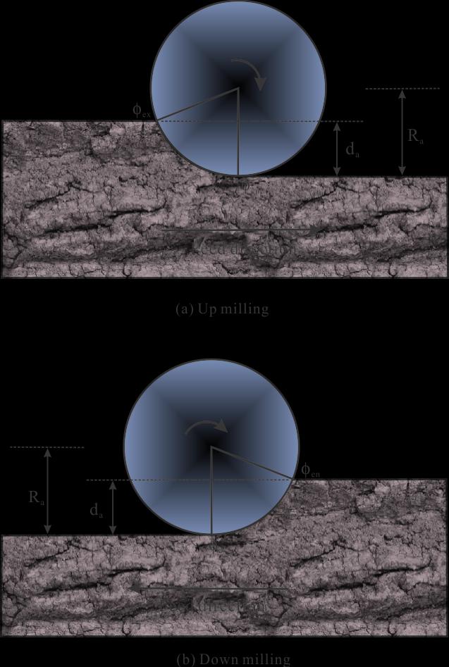
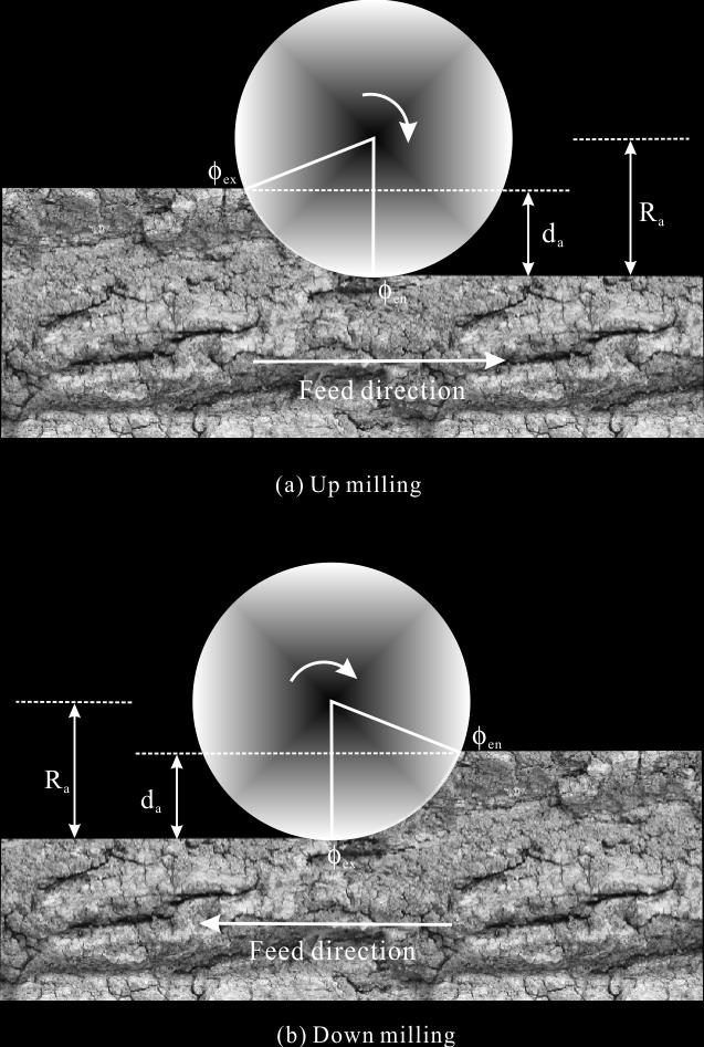
63 however, the coefficients that govern the force models are often restricted to a particular operation and the condition tested. In this chapter, an analytical force model for the helical end milling tool is developed by extending the orthogonal chip formation model developed in Chapter 3 to that for oblique cutting conditions. 4.2 Mechanics of milling process Milling is a process of removing material from the workpiece by feeding the work piece past a rotating multipoint cutter. Since the milling cutter is held in a rotating spindle with a fixed axis while the workpiece clamped on the table is moving linearly toward the cutter, the path of each of the milling cutter teeth forms an arc of trochoidal. As a result, varying but periodic chip thickness is generated at each tooth-passing interval. In practice, there are three types of milling operations commonly used in industry: 1. Up milling operation, also referred to as conventional milling, is characterized by the opposite direction of cutter rotation to the workpiece feed direction. In up milling, the formation of chip begins with a small load as the flute begins to cut and then increases gradually to the maximum right at the location where the flute exits the cutting region. See Figure

64 Figure 4-1 Up milling 2. Down milling operation, also known as climb milling, works in an inverse manner to up milling. That is, the cutter rotates in the same direction as the motion of the feed and the chip load decreases from a maximum value to zero during the cutter flute passing through the cutting region. See Figure

65 Figure 4-2 Down milling 3. Face milling operation, through which the milled surface results from the action of both the periphery and the face of the milling cutter. The entry and exit angles of the milling cutter relative to the work piece are nonzero. 50

66 Figure 4-3 Face milling The complexity of the milling tooth track makes the milling process inimical to mathematical treatments. On the other hand, the great similarities existing between milling and conventional oblique cutting operations could facilitate the analysis by treating the operation of every single flute as that of a single point cutting tool with relatively complicated geometry and kinematics. 51

67 4.3 Geometry of milling process The mechanics of chip formation is the most important aspect among all cutting operations. The analytical work on the geometry of the milling process was initiated by Martellotti [13, 14]. In his study, Martellotti identified feed per revolution, cutter radius as the crucial process and geometry parameters that decide the tool path. The author showed that the true path of the milling cutter tooth is a looped trochoid that can be represented by the equations below: f x Rsin 2 N y R1 cos (4.1) where f is the feed, N is RPM, R is cutter radius and is angular position of the cutter. The plus and minus signs are for up and down milling respectively. By closely investigating into the trochoidal path, Martellotti showed that the cutting tool, instead of being tangent, will enter the work material at a point higher than the previously machined surface, causing the well known phenomena--feed mark. It is so called because the distance between two adjacent feed marks equals the feed per tooth. Assuming the milling cutter is perfectly mounted, the author derived the approximate expression of the amplitude of the feed mark: 52

68 2 f t h (4.2) 8R Under the condition of tool eccentricity, a wavy machined surface will be generated with a frequency equal to that of the cutter rotation. He also illustrated that the severity of the feed mark could be diminished by decreasing feed per tooth and increasing cutter radius. Martellotti has also shown that the tooth path is almost circular for light feeds. In most real cutting condition, it is always true that feeds are much smaller than cutter radius. Therefore, the tooth path is simplified to a circle by Martellotti and the chip thickness equation was derived: t f sin (4.3) c Because of its reasonable accuracy, this equation has been used in almost all milling studies. Other than this, the average chip thickness, obtained by integrating Equation (4.2) over the rotational range from entry to exit angles and divided by the range of the cut, is derived as following: t c en ex t d c f Rd R en (4.4) 4.4 Mechanistic models for milling process 53

69 Milling force models generally fall into five categories according to increasing levels of sophistication and accuracy, as classified by Smith and Tlusty [15]: Average rigid force, static deflection model Instantaneous rigid force model Instantaneous rigid force, static deflection model Instantaneous force with static deflection feedback Regenerative force, dynamic deflection model The simplest milling force model is the average rigid force model which assumes that the average power consumed in the cutting is proportional to the material removal rate. The average cutting forces calculated this way are then applied to calculate static deflections of the tool treated as a cantilever beam. The work of Wang [16] is a standard example of this kind of model. Although the average rigid force model is a very good first approximation, as mentioned by Smith and Tlusty [15], it considers neither force variations inherent in intermittent cutting nor the influence of the tool deflection on the cutting forces. For more accurate predictions, the cutting forces at the tooth tip should be considered. The instantaneous rigid force model calculates the milling forces based on the instantaneous chip load. This way, the weakness cited from the average rigid model is basically overwhelmed. However, the deflection of the cutter is not considered in the force calculation. The instantaneous rigid force, static deflection model is developed 54

70 essentially based on the instantaneous rigid model and includes the static deflection calculation. It s called static deflection for the reason that the cutter deflection is considered as proportional to the cutting forces, without taking system inertia into consideration. The instantaneous force with static deflection feedback model is further improved from previous models by an iterative deflection calculation, in which the force and deflection are correlated. Finally, the regenerative force, dynamic deflection model combines all the advantages of previous models and further accounts for system inertia. The chatter and forced vibration phenomena associated with milling operations can also be accurately depicted by this model. In general, except the average rigid force, static deflection model, the other four kinds of models are based on the same root the instantaneous force. Because it is more realistic, most researches on the milling process have been following this idea. The pioneer work, based on Martellotti s analysis of the kinematics of the milling process, was started by Konnisberger and Sabberval [17, 18]. They studied tangential forces in detail and showed that two components of the cutting force vector could be predicted by using tangential and radial force components at any location on the cutting edge. The local tangential force is related to the instantaneous chip section and the local radial force is proportional to the tangential force: F K bt (4.5) x t t c 55

71 F K F (4.6) r r t where F t is tangential force, F r is radial force, b is the width of cut, t c is the instantaneous chip thickness calculated by Equation (4.3), K, t F r are defined as specific cutting forces, representing the cutting forces per unit area and vary with width of cut, depth of cut and feed. x is a process constant having common values of 0.7 to 0.8. The same method was utilized by Kline [19, 20] to study problems of cornering and forging cuts. He considered the milling cutter consisting of a series of orthogonal cutter disk segments. Each segment is rotating with respect to adjacent segment having different chip thickness. The total force acting on the cutter at a given angular position can be obtained by analysing local cutting model and summing up the forces acting on the individual cutter segments. Other than this, Kline considered the effect of cutter runout and incorporated it into the calculation of chip load. Furthermore, by assuming the cutter to be a cantilever beam, the tool deflection was calculated from the cutting forces predicted from the proposed model and was used to analyze the machined surface error. So far, the milling force model has developed to the third level, Instantaneous rigid force, static deflection model. Sutherland and Devor [21] improved Kline s method to predict cutting forces in flexible end milling systems. In this model, the effect of system deflections on the chip load was taken into account and the instantaneous chip thickness was solved based on the balance 56

72 between cutting forces and resulted cutter deflections. Later, based on the pioneer investigation on the end milling dynamics by Tlusty [22], Sutherland [23] further sublimated the model to the vertex, the Regenerative force, dynamic deflection model. Armarego and Deshpande [24] further studied and discussed the importance of both cutter runout and deflection on the cutting force fluctuations. In this study, three models, namely the ideal model for rigid cutter with no eccentricity, the rigid cutter eccentricity model and the more comprehensive deflection model, were assessed by experimental data. It s shown in this study that: All three models provide good predictions of average cutting forces and torques. Both the eccentricity and deflection models yield satisfactory results for force fluctuation predictions. The deflection model gives the best result in all cases, especially for the heavy cutting conditions under which undesirable cutter deflections commonly happen. However, the efficacy of this comprehensive model is traded off by the excessive computer processing time. Yucesan et. al [25-27] considered rake angle and evaluated the varying friction and pressure acting on the tool-chip interface. They developed a 3D cutting force prediction system for helix end milling process, in which cutting force coefficients ( K, chip flow angle ( c ) are considered to vary with cutter rotation angle: n K f ) and 57

73 df K da (4.7) n n c df K K da (4.8) f f n c where Kn and K f are specific cutting coefficients. The values of these specific energies depend on the tool and workpiece materials as well as tool geometry and cutting conditions. Yucesan and coworkers observed the high dependence of Kn and K f on the chip thickness ( t c ), cutting speed ( V ) and normal rake angle ( n ), the empirical equations relating the specific energies to them were developed: ln K a a ln t a lnv a ln a ln t lnv (4.9) n 0 1 c 2 3 n 4 c ln K b b ln t b lnv b ln b ln t lnv (4.10) f 0 1 c 2 3 n 4 c where a0 a4 and b0 b4are experimentally determined. Once the normal and friction forces are determined, they can be transformed into global coordinate system. Wang and Liang [28, 29] analysed the flat-end milling forces via angular convolution and established a close form angular convolution model for the prediction of cutting forces in the cylindrical end milling processes. Following these works, a numerous of mechanistic models have been developed based on either one or more works described above. All of these models are assuming that the 58

74 cutting forces can be related to the chip load through cutting specific energies which have to be determined from calibration experiments. 4.5 Analytical modeling of milling forces In the current study, the milling force simulation is based on the orthogonal force model developed in Chapter 3, so that experimental calibrations can be avoided. Geometric considerations must be made to use the analytical orthogonal model described in the previous chapter. As shown in Figure 4-4, the cutting flutes are modeled as discrete linear segments. Every flute on each segment can be treated as a single point cutting tool executing oblique cutting. Orthogonal cutting force model can be applied after the oblique-to-orthogonal conversion. The total force acting on the milling cutter can be found by summing up the forces acting on every flute segment of a given disk for a given tool angular position. 59

75 Figure 4-4 Segmented milling tool model Angular position In order to model the milling process, the position of every cutting point in the fixed tool coordinate system needs to be known. Referring to Figure 4-5, if i, j and k are defined as the flute number, the rotational increment number and the segment number respectively, every flute segment has a particular angular position for a set i-j-k combinations. The angular position of the cutter is denoted by: 60

76 ( j) j (4.11) where is the angular increment as the tool rotates. At the moment when the cutter starts to rotates, if the bottom of any of the flute is located at the position with zero rotation angle, the angular position of the bottom on any other flute can be defined as 2 i (4.12) n p d where n d is the total number of flutes on the cutter. The term 2 is the so-called pitch nd angle, the angular spacing between cutting flutes on an evenly fluted milling cutter. Because of the helix angle, angular positions of each point along a specific cutting flute in the tool coordinate system are different. This angular difference is defined as lag angle l. For a specific flute, the angular position at the k_th axial segment with respect to the bottom can be expressed in terms of the helix angle, hx a l tan( hx) k (4.13) R a In which a is cutting width of the elemental flutes (the axial depth of a disk element), R a is the radius of the milling cutter. 61

77 Combining these elements, a generalized expression of the angular position for an arbitrary cutting point in the tool coordinate system can be derived as 2 a ( i, j, k) j i tan( hx) k (4.14) n R d a Figure 4-5 Geometry of cutting tool 62

78 Chip load calculation Uncut chip thickness in milling operation can be defined as the portion left between two consecutive flute segments on the same disk. It s contributed by feed-per-tooth, but changes as the tool rotates. By assuming the tooth path to be circle, as suggested by Martellotti [13], the instantaneous uncut chip thickness, as shown geometrically in Figure 4-6, is calculated as following. t ( i, j, k) f sin i, j, k (4.15) u x This formula applies only to the condition under which the rotation axis of the spindle coincides with the geometrical axis of the milling cutter. In this case, each tooth has exactly the same radius and removes the same amount of material. 63

79 Figure 4-6 Chipload in end milling Cutter runout, referring to the state of tool cutting points rotating about an axis different from the geometrical axis, is a commonly existing phenomenon in machining. It can either be in the form of an offset, a tilt, or a combination of both. The type of runout involving a cutter axis offset is termed radial runout, while the type involving a cutter axis tilt is referred to as axial runout [30]. The magnitude of axial runout is usually small relative to the axial depth of cut, plus considering the difficulty of measurement, only radial offset will be considered in this study. 64

80 Figure 4-7 shows an end mill radial offset in a tool holder, where the runout angle run is defined to be the angle between the negative Y axis direction and the line connecting the spindle rotation center and the tool geometry center. is runout amplitude. When radial offset exists, each flute at every point along the axis of the cutter experiences a different chip thickness than predicted by Martellotti s approximate equation. The chip thickness generated by a specific cutting point depends on the effective radius of the flute and the effective radius of the other flutes as well. From the geometry in Figure 4-7, the following expression can be derived as the radial length from center of rotation to the cutting edge at given index numbers i and k. R k i R R i j k (4.16) 2 2 e(, ) a run 2 arun cos( run (, 0, )) (a) Schematic demonstration of radial runout 65

81 (b) Runout, cutter radius and effective cutter radius Figure 4-7 Radial offset runout of the milling cutter Once the effective radius is known, the chip thickness h at a specific angular position, as illustrated in Figure 4-8, is h( i, j, k) R ( k, i) d (4.17) e where d R ( k, i 1) f cos ( ( i, j, k)) f sin( ( i, j, k)) (4.18) e x x 66

82 Figure 4-8 Chip thickness diagram during end milling[19] To account for the situation when runout is very serious, Equation (4.17) can be modified as h( i, j, k) R ( k, i) R ( k, i m( i, j, k)) m( i, j, k) f sin( ( i, j, k)) (4.19) e e x m( i, j, k ) is an integer, counting from 1 to the value of the total flute number. For example, if the cutter contains 4 flutes, m( i, j, k) will count from 1 to 4. Every time if the previous cutting flute has removed the material, the value of m( i, j, k ) is set to 1 when calculating the uncut chip thickness for the current cutting flute at the same height. If the previous cutting flute failed to cut, the value of m( i, j, k) is increased by 1. In simulation, 67

83 for example, if the first flute cut, the second and the third flute have all failed to cut, the value of m( i, j, k) is set to Entry and Exit angle Because milling is an intermittent cutting process, an additional factor should be considered when modeling the milling process: whether or not the flute is engaged into cutting. The angular region in which the cutter is engaged in cutting is known as the immersion angle. The angles at which the flute begins to cut and exit to cut are called entry angle and exit angle, respectively. An illustration of the immersion angle for two main types of milling is shown in Figure

84 Figure 4-9 Demonstration of immersion angles 69

85 For up milling with a cutter radius zero and the exit angle ex is given by R a and radial depth of cut d a, the entry angle en is ex d Ra 1 a cos 1 (4.20) When the cutter offset exists, the approximation of zero entry angle may not be able to reflect the cutting geometry accurately. From the geometry of Figure 4-10, the general expression of the entry angle en can be derived by using the cosine law: ( i, j, k) cos en 2 m( i, j, k) Ra( k, i) fx m( i, j, k) f x Ra ( k, i) Ra ( k, i m( i, j, k)) (4.21) It can be seen that when runout doesn t exist, Equation (4.21) becomes en cos 1 f x 2Ra 2 (4.22) when Ra f x, en 0. 70

86 Figure 4-10 Immersion angles under the condition of runout For the down milling under the same cutting condition and with the same tool geometry, the entry angle and exit angle are both opposite to that in up milling Milling force prediction For oblique cutting, an additional force component F R exists due to the inclination angle i, as shown in Figure

87 Figure 4-11 Conventional Oblique Cutting Forces As stated in [10], for a given normal rake angle n and other cutting conditions, the forces F C and F t are almost independent of inclination angle i, and the chip flow angle c approximately satisfies Stabler flow rule [31], which can be expressed as: i (4.23) c It means that the cutting force F C and the thrust force F t in oblique cutting can be determined from the orthogonal theory by taking inclination angle as zero. By noting this 72

88 and realizing that the resultant force R must be acting in the plane containing tool-chip friction force and normal to the tool rake face, Hu et.al [32] developed an expression for F r in the following way: With regard to Figure 4-11, the resultant force R can be expressed in vector form R F cˆ Ftˆ F rˆ (4.24) C t r ĉ, ˆt, ˆr are unit vectors in cutting force, thrust force and radial force directions, respectively. The three unit vectors along the main cutting edge, normal to main cutting edge and the chip flow direction can, from geometry, be expressed in terms of the normal rake angle n and the chip flow angle c, as shown in the following equations. aˆ sin icˆ cos irˆ (4.25) bˆ sin cos icˆ cos tˆ sin sin irˆ (4.26) n n n qˆ sin aˆ cos bˆ (4.27) c c The unit vector normal to the rake face plane (i.e. the plane made by â and ˆb ) is found by the cross product of â and ˆb : 73

89 nˆ bˆ aˆ cos cos icˆ sin tˆ cos sin irˆ (4.28) n n n The unit vector normal to the plane where the resultant force R lies in (i.e. the plane made by ˆn and ˆq ) can be expressed in the same way: pˆ qˆ nˆ (sin i cos sin cos isin ) cˆ cos sin tˆ c n c n c (cos i cos sin sin isin ) rˆ c n c (4.29) Noting that R and ˆp are normal to each other, their inner product should be zero: pr ˆ 0 (4.30) Finally, the radial force F r is derived: F r FC sin i cos i sinn tanc Ft cos n tanc sin isin tan cos i n c (4.31) Once F r was obtained, based on the geometrical analysis on tube end cutting with side cutting angle C s (Figure 4-12) the cutting force components in the machine tool coordinate system was achieved: P F (4.32) 1 C P2 Ft cos Cs Fr sin Cs (4.33) P3 Ft sin Cs Fr cos Cs (4.34) 74

90 Where the positive directions of P 1, P 2 and P 3 are taken as the cutting velocity, negative feed and outward radial directions. Figure 4-12 Tube-end oblique cutting forces Utilizing the geometrical similarities between end tube turning and face milling, Young et.al [33] developed a face milling force model for single edge fly cut. The whole cutting process was modeled as an end tube turning process with a variable chip thickness. For the peripheral part of the end miller, the side angle then becomes: C s is 0. Equation (4.32~4.34) 75

91 P F (4.35) 1 C P F (4.36) 2 t P F (4.37) 3 r The ploughing force contributed by end cutting edge is normally disregarded since it is very small compared to the cutting force contributed by the peripheral flutes. After the forces are predicted for each segment, the total forces in the X, Y, Z directions are found by summing up the individual flute segment forces that have been transformed from the coordinate system defining oblique cutting. Equations (4.38) to (4.40) will be one part of solutions from Oxley s predictive machining theory for oblique cutting. F (,, ) cos( ) C i j k R (4.38) F ( i, j, k) Rsin( ) (4.39) t FC sin i cosi sin tan Ft cos tan Fr ( i, j, k) sin isin tan cos i (4.40) Equations (4.41) to (4.43) are the elemental forces acting on each flute segment of a defined disk at a given rotational position. 76

92 F ( i, j, k) F cos F sin (4.41) x C ijk t ijk F ( i, j, k) F sin F cos (4.42) y C ijk t ijk F ( i, j, k) F (4.43) z r Equations (4.44) to (4.46) are total forces in X, Y, Z directions at a given rotational position. x Nd K x (4.44) i1 k1,, F j F i j k y N f K y (4.45) i1 k1,, F j F i j k z N f K z (4.46) i1 k1,, F j F i j k The flow chart is shown in Figure

93 Figure 4-13 Flow chart of analytical simulation of end milling process 78

94 Results and verification In order to verify the predictive milling force model, a set of experiments has been carried out on AISI 1045 with CNC milling machine under 4 combinations of different cutting conditions. A HSS flat-end mill with four flutes, 12.7mm diameter, 5 o normal rake angle and 30 o helix angle was used in the experiment. A list of specific cutting conditions for the tests is shown in Table 4-1.The material used in the experiments is AISI 1045 prepared in a block shape. Six holes are drilled into the block in order to be attached to the dynamometer. The chemical composition of AISI 1045 is listed in Table 4-2. The comparisons of predicted cutting force profiles based both on the original Oxley s machining theory and the one modified with Johnson-Cook material model, with data from milling test on AISI 1045 are shown in Figure 4-14 and Figure The modified model is further verified by comparing the simulated results with published data for AL T6 [34], Ti-6Al-4V [26] and AL-7075-T6 [27]. The cutting conditions are listed in Table 4-3, Table 4-4 and Table 4-5. The comparisons are shown in Figure 4-16, Figure 4-17 and Figure 4-18 respectively. F x, F y and F z represent forces in the feed, normal to the feed and the axial directions. Each plot pictures the cutting force profiles for one revolution of the milling cutter. 79

95 Table 4-1 Cutting conditions for end milling of AISI1045 Material: AISI1045 Exp.No Feed Feed rate Cutting speed Spindle speed Axial cutting depth Type of milling Radial Runout depth Runout angle (mm/min)(mm/tooth) (m/min) (RPM) (mm) (mm) (mm) (degree) down down down down Table 4-2 Chemical composition of AISI1045 Carbon (C) Manganese (Mn) Silicon (Si) Phosphorus (P) Sulfur (S) max max 80

96 Forces (N) Forces (N) OX-AISI1045-Test#1 experimental predicted Fy Fx Fz Rotation angle (degree) (a) Test experimental OX-AISI1045-Test #2 predicted Fy Fx Fz Rotation angle (degree) (b) Test 2 81

97 Forces (N) Forces (N) experimental OX-AISI1045-Test#3 predicted 400 Fy Fx Fz Rotation angle (degree) (c) Test experimental OX-AISI1045-Test #4 prediected 400 Fy 200 Fx 0 Fz Rotation angle (degree) (d) Test 4 Figure 4-14 Comparison of predicted cutting forces based on Oxley s original model with measured data for AISI

98 Forces (N) Forces (N) experimental AISI1045-Test #1 predicted 400 Fy Fx Fz Rotation angle (degree) (a) Test AISI1045-Test #2 800 experimental predicted 600 Fy Fx Fz Rotation angle (degree) (b) Test2 83

99 Forces (N) Forces (N) experimental AISI1045-Test #3 predicted Fy Fx -100 Fz Rotation angle (degree) (c) Test AISI1045-Test #4 600 experimental predicted Fy Fx Fz Rotation angle (degree) (d) Test 4 Figure 4-15 Comparison of predicted cutting forces based on modified Oxley s model with measured data for AISI

100 Table 4-3 Cutting conditions for end milling of Al6061-T6 Material: AL6061-T6 Exp.No Rake angle Feed rate Cutting speed Helix angle Axial Type cutting of depth milling Radial depth Runout Runout angle (degree) (mm/tooth) (degree) (RPM) (mm) (mm) (mm) (degree) down down down down Table 4-4 Cutting conditions for end milling of Ti-6Al-4V Material: Ti-6A1-4V Exp.No Rake angle Feed rate Cutting speed Helix angle Axial Type cutting of depth milling Radial Runout depth Runout angle (degree) (mm/tooth) (degree) (RPM) (mm) (mm) (mm) (degree) up N/A up N/A 85

101 Forces (N) Table 4-5 Cutting conditions for end milling of Al-T7075 Material: T7075 Aluminum alloy Exp.No Rake angle Feed rate Helix angle Spindle speed Axial cutting depth Type of milling Radial Runout depth Runout angle (degree) (mm/tooth) (degree) (RPM) (mm) (mm) (mm) (degree) up N/A up N/A experimental AL6061-Test #1 predicted Fy Fx Fz Rotation angle (degree) (a) Test 1 86

102 Forces (N) Forces (N) 600 AL6061-Test #2 500 experimental 400 predicted 300 Fy Fx -100 Fz Rotation angle (degree) (b) Test AL6061-Test #3 200 experimental predicted Fy 50 Fx 0-50 Fz Rotation angle (degree) (c) Test 3 87

103 Forces (N) Forces (N) experimental AL6061-Test #4 predicted Fy Fx Fz Rotation angle (degree) (d) Test 4 Figure 4-16 Comparison of predicted cutting forces based on modified Oxley s model with measured data for AL6061-T experimental Ti6Al4V-Test #1 predicted Fy Fx Fz Rotation angle (degree) (a) Test 1 88

104 Forces (N) Forces (N) 500 Ti6Al4V-Test #2 400 experimental predicted Fy Fx Fz Rotation angle (degree) (b) Test 2 Figure 4-17 Comparison of predicted cutting forces based on modified Oxley s model with measured data for Ti6Al4V experimental AL7075-Test #1 predicted Fy Fx Rotation angle (degree) Fz (a) Test 1 89

105 Forces (N) experimental AL7075-Test #2 predicted Fy Fx Fz Rotation angle (degree) (b) Test 2 Figure 4-18 Comparison of predicted cutting forces based on modified Oxley s model with measured data for AL7075 As shown in these helix end milling force profiles, several features can be noticed. The cutting forces in all three directions increase gradually to the peak values, instead of jumping directly to the peak. This is due to the effect of the helix angle. Without helix angle, a specific cutting flute will engage into material at the same time. Because of the lag angle caused by the helix angle, the cutting flute will engage into material gradually from the bottom up to the height of the axial depth of cut. Therefore, the peak force values are reached at the moment when the total chip thickness contributed by all the elements along the helix flute is the maximum. The larger the helix angle, the later the peak value be achieved. 90

106 F y acts constantly in positive direction. This is obvious because the force components contributed by both during the whole cutting engagement. F c and F r are all in the positive Y direction F x oscillates from negative to positive as the flutes engage and disengage. This feature is contributed to the opposite x components of the F c and F r. When the cutting flute begins to cut, the direction of F c is perpendicular to the feed direction, while F r acts in the same direction as the feed. Therefore, the negative feed direction. As the tool rotates, the domination of by F c gradually. It is easy to find that the contribution from F x acts in F r is attained F c and F r will reach the balance at the rotation angle of /4, meaning that F x will be zero at this moment if Fc F. The fact that for most cutting conditions and materials r F c Fr is always true makes x F reach zero earlier. The effect of runout can be seen vividly in all the plots. The first flute experiences the largest chip thickness and the third flute experiences the smallest. More importantly, it can be seen that it is the cutting radius difference, not the effective cutting radius itself that contributes the effect of runout. Referring to the runout geometry in this experiment, the order of the effective cutting length from high to low for the four cutting flutes is , while the order of peak forces is

107 This fact indicates that the fourth flute experienced larger chip thickness than the second flute did, although the second flute has a longer effective cutting radius. The reason is that the second flute has a shorter effective radius than the first one, so a portion of chip thickness supposed to be left for it is robbed by the first flute. On the other hand, although the fourth flute has a shorter effective length than the second one, it enjoyed a large portion of chip thickness left by the shortest flute, the third flute. The conclusion could be reached that the radial runout offset redistributes the share of chip load. The MMR might not be influenced so much. All these features discussed above are captured very well by the developed force model. By using Johnson-Cook material model to represent material behaviour, almost the same results are achieved. 4.6 Conclusion In this chapter, an analytical end milling force model was developed and verified. An analysis of the cutting forces for helix end milling processes was performed and an application of Oxley s orthogonal machining theory to the end milling force prediction was achieved. The end milling force profile under the condition of cutter offset is able to be simulated by the model, with the input data of cutting conditions, machine tool geometry and the work material properties. 92

108 CHAPTER 5. PHENOMENOLOGICAL MODELING OF DEFORMATION DURING METAL CUTTING Equation Chapter (Next) Section Introduction In Oxley's machining theory, the efforts have been made to address work hardening and thermal softening effects and allow the material to flow continuously through an openedup deformation zone. However, the strain, strain rate and temperature were calculated based on the average values. The distributions of these processing parameters, which are essential to describe the continuous flow, were not taken into account. In particular, the hodograph was adopted from the single shear plane model, in which the velocity field allowing for the continuous deformation was not described, and the issue of velocity discontinuity has not been resolved. In this chapter, the prediction of various processing parameters is based on the methodology developed in Chapter 3, while the strain, strain 93

109 rate and velocity fields in the primary shear zone that allows the continuous deformation has been analyzed, in an attempt to provide an improved insight into the flow behavior in the primary shear zone. With the detailed analysis on the boundary conditions of the velocity and shear strain rate fields, the thick equidistant parallel-sided shear zone model was revisited. A more realistic nonlinear shear strain rate distribution has been proposed under the frame of non-equidistant primary shear zone configuration, so that all the boundary conditions can be satisfied. 5.2 Velocity, strain and strain rate during chip formation In Oxley's parallel-sided shear zone model shown in Figure 2-10, the shear zone is bounded by the lower boundary CD where the deformation starts and upper boundary EF where the deformation ends. An approximation was made where CD and EF are assumed to be parallel to and equidistant from AB. The hodograph utilized in the analysis was the same as that in single shear plane model without considering the material continuity. In addition the total shear strain at upper boundary EF was calculated in a way identical to that proposed by Merchant [2] and the strain at AB was taken as one half of the total strain, as shown in Equation (2.27). This result is the direct consequence of the equidistance assumption and the absence of the strain distribution expression across the primary shear zone. 94

110 Based on the experimental data, Oxley [10] showed that the strain rate distribution is a bell-shaped curve through the primary shear zone and the maximum shear strain rate occurs at AB. However, the strain rate distribution was not formulated or utilized in the analysis and instead the shear strain rate at AB is used and calculated by Equation (2.28). Based on the engineering plasticity, several researchers reevaluated the orthogonal metal cutting mechanics in the primary shear zone [35-38]. In their studies, the coordinate system is commonly set based on the shear angle, as shown in Figure 5-1, where the x direction is set along the shear zone boundaries and the y direction is perpendicular. Figure 5-1 Simplified non-equidistance primary shear zone 95

111 Since the boundaries CD and EF are assumed to be slip lines, Geiringer s Equation holds: dv V d 0 (5.1) x y Because the slip lines are simplified to be straight, Equation (5.1) implies that is constant along x direction, or V x x 0 (5.2) The continuity of incompressible plastic materials requires V x V y x y 0 (5.3) Equation (5.2) and (5.3) imply that the velocity component normal to the shear plane AB is constant across the parallel-sided shear zone and therefore all the analysis in the primary shear zone can be considered as one dimension. For a given cutting speed, the entry and exit boundary conditions for the velocity field can be obtained. Vx 1 Vx U cos y0 Vx2 Vx U sin tan yh Vy Vy y U sin (5.4) 96

112 The velocity discontinuity is defined as the difference between and [37]: * cos Vx Vx2 Vx 1 U cos (5.5) It should be noted that equals in magnitude. Comparing Equation (5.5) and (2.28), it also can be seen that in Eq. (2) is actually the mean shear strain rate of the primary shear zone, since the mean shear strain rate is expressed as: * Vx 2 Vx 1 Vx m (5.6) h h In this study, it should be noticed that the simple shear is assumed to occur along parallel planes and therefore the main frame remains unchanged during plastic deformation. Thus, the shear strain rate can be related to the shear strain and velocity, as shown in Equation (5.7) and (5.8) respectively. Vy Vx dvx x y dy (5.7) d dy d V y dt t y dt dy (5.8) Substituting Equation (5.7) into Equation (5.8) and integrating with respect to y, the relation between velocity and shear strain field can be expressed such that: 1 y Vx y cot (5.9) V y 97

113 As can be seen from Equation (5.4), as long as the shear angle is greater than the rake angle, the sign of are opposite, indicating that there must be a plane, in the primary shear zone, at which the tangential velocity is zero. This plane is the potential sliding plane [37] and it is therefore reasonable to assume it as the main shear plane, at which the discontinuity of the shear stress and velocity could take place and the shear strain rate is the maximum. Many researchers observed from quick stop analysis that the primary shear zone is divided by the main shear plane into two unequal regions. The lower region (from CD to AB) is wider than the upper region (from AB to EF). The detailed review can be found in the work by Tounsi, et al. [35]. Astakhov, et al. [37] further realized that in the lower wide region the velocity ratio changes with lower rate, but in the upper narrow region it changes with higher rate. They also observed based on experimental data that the non-uniform distribution of the tangential velocity in the primary deformation zone is proportional to at moderate cutting speed. From the above analysis, if is defined as the proportion of the lower part to the total width of the deformation zone, the boundary conditions of the velocity and shear strain rate fields in the primary shear zone are as follows: 1) The primary shear zone is unequally divided by the main shear plane AB ( ). 98

114 2) The quantities defining plastic deformation depends only on y, the direction perpendicular to the main shear plane. 3) The tangential velocity is and at lower and upper deformation boundaries respectively (Equation (5.4)). 4) The tangential velocity is zero at main shear plane AB. V x y 0 (5.10) h 5) The shear strain rate at main shear plane AB is the maximum and is zero at lower and upper boundaries. yh AB (5.11) (5.12) y (5.13) y h 6) Since the material particles move toward the primary shear zone with constant speed, the change rate of the velocity and the corresponding shear strain rate are zero before the lower boundary CD is reached. Similarly, after passing through the upper boundary EF, the strain rate of the particles reduces to zero again. If the strain rate distribution is assumed to be represented by a smooth differentiable curve across the entire primary shear zone from CD to EF (including both inner sides and outer sides), there must be an extremely thin buffer zone around CD and EF, in which the gradient of the shear strain rate with respect to y is zero. In 99

115 this study, the locations around CD and EF that the gradient of the shear strain rate reaches zero are defined as lower and upper boundaries respectively. Furthermore, the assumed differentiable nature of the curve leads to the fact that the gradient of the shear strain rate with respect to y is also zero at the main shear plane AB where the shear strain rate reaches the maximum, i.e., d dy yh 0 (5.14) d dy y0 0 (5.15) d dy yh 0 (5.16) 7) A fourth order polynomial curve in terms of y and h could describe the velocity distribution in the primary shear zone for moderate cutting speed [37]. According to these characteristics and boundary conditions, the pattern of velocity and shear strain rate distribution may be illustrated in Figure 5-2. Based on these conditions and considering a 4 th order polynomial curve is possible to describe the velocity field for moderate cutting speeds, the following piecewise strain rate distribution is proposed. 2 2 y h Dy y Ehy + Fh 0 γ = d h - y y + ehy + fh 2 2 y h h (5.17) 100

116 In which are coefficients that need to be determined. It can be seen Equations (5.12) and (5.13) are satisfied by Equation (5.17). The gradient of shear strain rate through the primary shear zone can be expressed as: D y Ehy Fh y h d dy 2 2 d 3y 2 e 1 hy f e h y h h (5.18) Considering the boundary conditions of Equation (5.4), the velocity field can be obtained by the spatial integration of shear strain rate. V x h dy Vx 1 D y Ehy Fh y h y 2 4ehy dy Vx2 d h y e 6 f h h (5.19) 101

117 Figure 5-2 Demonstration of the distribution of tangential velocity and shear strain rate in the primary shear zone For h, in order to satisfy Equation (5.15), F 0 (5.20) In order to satisfy Equation (5.14) F 3 2E (5.21) 102

118 Substituting Equation (5.20) into (5.21), 3 E (5.22) 2 In order to satisfy Equation (5.11), E hd D h 3 3 AB 2 3 (5.23) From Equations (5.21) and (5.23), the constants can be expressed in terms of and h, as shown in Equation (5.24). 2 D AB (5.24) 3 3 h In order to satisfy Equation (5.10), the shear strain rate at main shear plane AB can be obtained. AB 2V x1 h (5.25) Similarly, from conditions(5.11),(5.14) and (5.16) for h, coefficients can be obtained. 103

119 d h 3 2 AB 1 3 (5.26) 3 1 e (5.27) 2 f 3 1 (5.28) 2 Satisfying Equation (5.10) by Equation (5.19), the shear strain rate at AB can also be calculated as AB 2V x 2 1 h (5.29) The combination of Equation (5.25) and (5.29) lead to the expression of. V V V V V x1 x1 * x1 x2 x (5.30) Considering and, and can finally be expressed as cos cos (5.31) cos 104

120 AB * Vx 2 2m (5.32) h Finally, replacing in Equations (5.17) and (5.19), shear strain rate and velocity fields can be obtained, as shown in Equations (5.33) and (5.34) y AB 2 y 3h 2y AB 3 3 h 2 h y h 3h 2y y 0 h y h h (5.33) V x y y 2hy h Vx 1 y h h y 2h 2h y 6h y 2h 6h y Vx2 AV y 4 h h 4 h 1 (5.34) where A V (5.35) 105

121 Using the velocity distribution in Eq. (20) the shear strain distribution in Eq. (11) can be determined and the corresponding shear strain at the main shear plane can be given by: AB cot yh EF (5.36) Figure 5-3 shows the effect of shear angle on the proportion factor for different values of rake angle. From the illustrated results, in order to make the main shear plane right at the middle of the shear zone a combination of large negative rake angle and large shear angle must occurred. However, this circumstance could hardly happen since cutting tools with large negative rake angle result in the severe plastic deformation leading to large chip ratio and therefore small shear angle. On the other hand, could be equal to or even greater than one if a large positive rake angle is used and very small shear angle occurred simultaneously. However, this situation is also unrealistic because large shear angles are always the consequences of using cutting tools with large positive rake angles, at least when continuous chip formation is assumed. Therefore, from the above analysis, always falls into the range between 0.5 and 1. This observation is in agreement with reported experimental observations [35] that the entry zone (from CD to AB) was found to be wider than the exit zone (from AB to EF). 106

122 Proportion of the PSZ (λ) =-20 =-10 =0 =10 =20 AB is in the middle of Shear angle φ (degree) Figure 5-3 Primary shear zone proportion Figure 5-4~Figure 5-6 show the distributions of the shear strain rate, tangential velocity and the shear strain across the shear zone for different values of primary shear zone thickness. One can see from the illustrated results that the proportional factor, when and, which is unrealistic. In a more realistic case for shear angle ( when cutting with a zero rake, ) the obtained proportional factor, indicating that the main shear plane AB is closer to the upper deformation boundary and implying a higher rate of velocity changes in the upper region. This is in accordance with the experimental observation in [37]. Also, It can be seen from these figures that for the same total shear strain, the thickness of the primary shear zone (or ) determines how fast the plastic deformation process proceeds. The thinner the primary shear zone thickness, the faster the progress of the deformation, ie. higher strain rate. 107

123 shear strain rate (1000/S -1 ) shear strain rate (1000/S-1) U=200 m/min φ=30 O α=-5 O λ=0.7 h=20 m h=30 m h=50 m Distance from the shear plane AB (μm) AB (a) Asymmetric distribution U=200 m/min φ=40 O α=-10 O λ=0.5 AB h=20 m h=30 m h=50 m Distance from the shear plane AB (μm) (b) Symmetric distribution Figure 5-4 Shear strain rate distribution through the primary shear zone 108

124 Tangential Velocity (m/s) Tangential Velocity (m/s) U=200 m/min φ=30 O α=-5 O λ= AB Distance from the shear plane AB (μm) h=20 m h=30 m h=50 m (a) Asymmetric distribution 3 AB U=200 m/min φ=40 O α=-10 O λ=0.5 h=20 m h=30 m h=50 m Distance from the shear plane AB (μm) (b) Symmetric distribution Figure 5-5 Tangential velocity distribution through the primary shear zone 109

125 Shear strain Shear strain AB U=200 m/min φ=30 O α=-5 O λ=0.7 h=20 m h=30 m h=50 m Distance from the shear plane AB (μm) (a) Asymmetric distribution AB U=200 m/min φ=40 O α=-10 O λ=0.5 h=20 m h=30 m h=50 m Distance from the shear plane AB (μm) (b) Symmetric distribution Figure 5-6 Shear strain distribution through the primary shear zone 110

126 5.3 Results and discussion In this chapter, Oxley s machining theory has been modified to consider the shear strain and strain rate distribution across the primary shear zone. The presented analysis based on the velocity and strain field for the incompressible material reveals that the location of the main shear plane is not right in the middle of the primary shear zone, but can be related to the material properties and cutting conditions. In this section, the comparison will be made between the current and Oxley s results when predicting process parameters such as cutting forces, chip thickness and secondary shear zone thickness. The work materials used for comparison in this work are 0.20% carbon steel and AISI 1045 steel. The experimental data for 0.20% carbon steel is adopted form [10] and that for AISI 1045 steel is adopted from [39]. Figure 5-7 and Figure 5-8present the predicted and measured machining forces and chip thickness for 0.20% carbon steel. The marks with the solid fill are the data when builtup-edge were observed. It can be seen that there is no significant difference between the current and Oxley s predictions. This may be explained by the fact that the cutting forces are determined by both work hardening and thermal softening effects. With the unequal distance primary shear zone, the predicted shear strain, shear strain rate and temperatures in the current study are all higher than that by Oxley s original method. So that the resultant effect of work hardening and thermal softening makes the results similar. However, the uncertainty about the location of the main shear plane is eliminated 111

127 Cutting Force (N) in the current work. Instead of, the predicted location of the main shear plane is closer to the upper boundary of the primary shear zone, which was discussed earlier, and it tends to move towards the lower boundary as the cutting speed increases, as shown in Figure 5-9. Figure 5-9 (a) presents the predicted thickness of the primary shear zone. Oxley's predictions are quite similar to that in the current study; they both decrease with the increase in cutting speed and uncut chip thickness. However, the uncertainty about the location of the main shear plane is eliminated in the current work, as can be seen in Figure 5-9(b) that varies with the cutting speed and uncut chip thickness. The increase in both cutting speed and the uncut chip thickness decreases, indicating that the deformation process will be more symmetric when cutting material with high feed and high cutting speed Oxley's prediction Current prediction Experiment t 1 =0.5mm t 1 =0.25mm t 1 =0.125mm Cutting Speed (m/min) (a) Cutting force 112

128 Chip thickness (mm) Thrust Force (N) Cutting Speed (m/min) Oxley's prediction Current prediction Experiment t 1 =0.5mm t 1 =0.25mm t 1 =0.125mm (b) Thrust force Figure 5-7 Machining forces for 0.20% carbon steel: Oxley's prediction Current prediction Experiment t 1 =0.5mm t 1 =0.25mm t 1 =0.125mm Cutting Speed (m/min) Figure 5-8 Chip thickness for 0.20% carbon steel: 113

129 Proportion factor of PSZ (l) PSZ thickness (mm) Oxley s prediction Current prediction t 1 =0.5mm t 1 =0.25mm t 1 =0.125mm 6E Cutting Speed (m/min) (a) Thickness of the primary shear zone t 1 =0.125mm t 1 =0.25mm t 1 =0.5mm Cutting Speed (m/min) (b) Proportion factor ( ) of the primary shear zone Figure 5-9 Predicted thickness and the proportion factor of the primary shear zone for 0.20% carbon steel: 114

130 Figure 5-10 presents the thickness of the secondary shear zone at various uncut chip thickness. As can be seen, the predicted values in the current work are lower than that predicted by Oxley's model when cutting speed is low and they tend to coincide at high cutting speeds, particularly for the high feed rate. The difference between the current and previous predicted results can be explained by the dependence of the thickness of the secondary shear zone on the severeness of the further shear at the chip-tool interface. The more severe the shearing, the thinner the secondary shear zone. In order to balance the resultant force transmitted from the primary shear zone, the shear stress at the chip-tool interface and on the main shear plane are interrelated, and is affected by the combined effects of work hardening and thermal softening. Since in the current study, the predicted shear strain, strain rate and temperature at main shear plane are higher than Oxley s prediction. The lower cutting speed results in the lower temperature, so that the effect of work hardening predominates on the main shear plane. Therefore, when cutting speed is low, the currently predicted shear stress is higher and the corresponding thickness of the secondary shear zone is lower. When the cutting speed increases, the resulted high temperature counteracts the effect of work hardening and makes the magnitude of similar to that predicted by Oxley. Consequently, compared to Oxley s prediction, the thickness of the secondary shear zone is lower in the current study, especially at lower cutting speeds. However, it is important to note that the current prediction shows improved agreement with the mean value of the experimental data. 115

131 SSZ thickness (mm) SSZ thickness (mm) Oxley's prediction Current prediction Experiment Cutting Speed (m/min) (a) Oxley's prediction Current prediction Experiment Cutting Speed (m/min) (b) 116

132 SSZ thickness (mm) Cutting Speed (m/min) Oxley's prediction Current prediction Experiment (c) Figure 5-10 Secondary shear zone thickness for 0.20% carbon steel: Figure 5-11shows the predicted shear strain rate, shear strain and velocity distributions across the primary shear zone. As can be seen in Figure 5-11(a), the location of the main shear plane AB is shifting towards the lower boundary of the plastic deformation zone when cutting speed increases. Moreover, not only the average magnitude, but also the gradient of the shear strain rate and tangential velocity is increased, reflecting the fact that the time left for the gradual plastic deformation is less during cutting with higher speed and the chip formation process tends to be localized at the main shear plane. On the other hand, the total shear strain at the exit boundary decreases with the increase in the cutting speed, as shown in Figure 5-11(b). In fact, the total shear strain is the accumulation of the local shear strains on all the layers across the plastic deformation 117

133 Shear strain rate (S-1) zone. The lower cutting speed provides more time and space for the work material to respond to the external force, as can be seen in Figure 5-11(c). As the result, the width of primary shear zone is increased by the decrease in the cutting speed, indicating that more material particles are involved in the plastic deformation and contribute shear strains to the total shear strain. Consequently, the developed strain energy is larger and the cutting energy needed to remove the material is higher. This can be reflected from the higher machining forces at lower cutting speeds. 6,000 5,000 4,000 3,000 2,000 1,000 U=100 m/min U=200 m/min U=400 m/min Entry boundary Exit boundary 0 AB Nondimensional distance from the entry boundary of the primary shear zone (a) Shear strain rate distribution 118

134 Tangential Velocity (m/s) Shear strain U=100 m/min U=200 m/min U=400 m/min Distance from the shear plane AB (mm) AB (b) Tangential velocity distribution U=100 m/min U=200 m/min U=400 m/min -6 AB Distance from the shear plane AB (mm) (c) Shear strain distribution Figure 5-11 Predicted shear strain rate, shear strain and velocity distributions across the primary shear zone for 0.20% carbon steel: 119

135 Furthermore, another set of data was selected from the experimental work done by Ivester et al [39], to evaluate the effect of modifications under various cutting conditions. The cutting conditions are listed in Table 5-1. In their work, the orthogonal cutting tests were conducted form 4 laboratories using the same cutting tools. The upper bound (solid line) and the lower bound (dash line) of the measured forces are shown in Figure It can be seen again that no distinguishable difference can be found between two models. One can see that the predicted cutting forces basically fall into the boundaries. However, most thrust forces are underestimated. This may be attributed to the assumption of the perfectly sharp tool applied in the current study. Table 5-1 Orthogonal Cutting Conditions For AISI 1045 (w=1.6 mm) [39] Test V (m/min) t 1 (mm) α (degree)

136 Thrust Force (N) Cutting Force (N) Oxley prediction Current prediction Test Number (a) Cutting force Oxley prediction Current prediction Test Number (b) Thrust force Figure 5-12 Comparison of predicted machining forces with experimental data [39] for AISI 1045 steel: 121

137 5.4 Conclusion In this chapter, an attempt has been made to modify Oxley s machining theory by considering the effect of shear strain, strain rate distributions. A more realistic bellshaped strain rate distribution through the primary shear zone was proposed in an attempt to satisfy all the velocity field boundary conditions. The proportion parameter ( ) of the primary shear zone was determined as part of the solution, so that Oxley s equidistance assumption was eliminated. The effect of the modification made to Oxley s model was evaluated in terms of machining forces, chip thickness and secondary shear zone thickness. It has been found that the main shear plane, at which the shear strain rate reaches the maximum, hardly locates at the middle of the primary shear zone in the moderate range of cutting speed. Instead, it is closer to the upper boundary of the plastic deformation zone and dependant on where the tangential velocity of work material particle changes direction. Although the modified model predicts higher strain, strain rate and temperature at the main shear plane, the machining forces are quite similar to that by Oxley s original model. However, this coincidence is encouraging since the modified model is more phenomenological and several uncertainties are eliminated from the previous model. 122

138 CHAPTER 6. IDENTIFICATION OF MATERIAL CONSTITUTIVE EQUATION FOR METAL CUTTING Equation Chapter (Next) Section Introduction With the development of computer technology, the numerical methods, such as Finite Difference and Finite Element Analysis have been widely applied to the simulation of metal cutting processes. One of the obstacles that hinder the further application of CAE technology is the successful identification of the set of parameters in the material constitutive model. Furthermore, plasticity based analytical modeling of metal cutting process, as the one in the current study, highly depends on the accuracy of material model as well. Therefore, the accurate identification of the material parameters under the conditions similar to that encountered in metal cutting is crucial. Split Hopkinson Pressure Bar (SHPB) tests have been commonly used to obtain material constants at 123

139 various strain rate and temperature levels. However, much higher strain rate are commonly observed in real metal cutting process, and due to the extremely high heating rate during chip formation, there is no enough time for complete phase transformation, anneal softening, age hardening, or even blue brittleness effects to occur[40]. Inverse analysis applies optimization techniques to identify the material parameters by minimizing a particular norm of the difference between the calculated and experimental machining data, in an attempt to reach the extreme conditions (high strain, strain rate and temperature) encountered in metal chip formation process. Shatla et al [41] developed a methodology using OXCUT and 2D orthogonal slot milling test to obtain modified Johnson-Cook parameters. A multi-directional Downhill Simplex Algorithm was chosen to minimize the sum of deviations between the measured and calculated cutting and thrust forces. This methodology was further improved by Sartkulvanich et al [42] by measuring the thickness of primary and secondary shear zone thickness. The Johnson- Cook model for low carbon steels was modified to take the blue brittleness effect into account. Chandrasekaran and M Saoubi [43] used milling test to obtain Johnson-Cook constants as well. In their study, the data from SHPB tests was applied as starting point for least square search. Instead of cutting and thrust forces, the shear stress along the primary deformation zone was used to create the objective function, making the inverse analysis at the tool-chip interface unnecessary. Lei et al [44] calculated strain rate based on a triangular shear zone. The shear plane temperature was measured with the infrared camera through a small opening in the shield placed in front of the cutting tool, and the 124

140 angle formed between upper/lower boundary and the shear plane AB was measured from a photograph of the microstructure associated with the side of the chip. Tounsi et al [35] re-evaluated the velocity field, stress and strain states in the primary shear zone based on the plastic incompressibility. In their study, the primary shear zone was assumed not equi-distant and the thickness was assumed one half of the feed rate. An expression was derived to define the portion of primary shear zone in terms of shear angle and tool rake angle. Based on the developed strain, strain rate and the temperature along shear plane AB, a least-square approximation technique was applied to determine the Johnson-Cook constants. Pujana et al [40] applied inverse analysis to the secondary shear zone. With the measured tool-rake face temperature and the thickness of secondary shear zone, the Johnson-Cook constants were tuned based on the experimental characterization results. Ozel and Zeren [45] applied Gauss-Newton algorithm to obtain Johnson-Cook constants by utilizing measured forces and chip thickness obtained through orthogonal cutting tests. In their methodology, the assumption of the primary shear zone thickness was eliminated and the shear strain rate constant was obtained by the inverse analysis of Oxley s theory. In these optimization methods the proper starting points are needed. Improper starting points could lead to local optimum instead of global optimum. In order to overcome this obstacle, in this Chapter, an attempt has been made to develop a Genetic Algorithm for the identification of Johnson-Cook parameters under the conditions encountered in metal 125

141 cutting process. The methodology is based on the methodology of the primary shear zone developed in the previous chapter, in conjugation with orthogonal cutting tests. 6.2 Inverse analysis in the primary shear zone First of all, the cutting force, thrust force and chip thickness should be measured from experiment. The shear angle can then be determined. tan 1 2 t1 cos t t t sin (6.1) Secondly, the shear strain, shear strain rate and temperature can be calculated with equations (5.36), (5.32) and (2.32), and substituted into Johnson-Cook equation (3.1), to obtain the calculated flow stress. C0 has to be known in prior to calculate shear strain rate. From the slip line field analysis described in chapter 3, C0 can be expressed in terms of equivalent flow stress, n 3 A B AB C0 PA PB (6.2) n 2 n AB AB where PA can be calculated from Equation (3.12) and PB can be derived based on the known experiment data. 126

142 2sin PB PA Fc sin Ft cos tw 1 (6.3) On the other hand, the average flow stress on the shear plane can be obtained by force relations with the measured data, 3 sin exp Fccos Ftsin (6.4) wt 1 Finally, in order to identify the five flow stress parameters, an error function may be built to be minimized through a certain optimization algorithm, as shown in Equation(6.5). 2 N 1 cal A, B, n, C, m min 1 (6.5) N i1 AB To carry out the minimization of Equation (6.5), a Genetic Algorithm was developed to carry out the minimization and will be introduced in the next section. 6.3 Development of Genetic Algorithm for the system identification Genetic algorithm (GA), first developed by Holland [46], is a selective random search algorithm designed to achieve a global optimum within a large space of solutions. It resembles the process of natural selection in search for better characteristics within a changing population. GA has been used as efficient optimizers and employ the concept 127

143 survival of the fittest among string structures. The initial solutions of GA algorithm are usually randomly generated and form the current generation. The current generation goes through the following procedure and generates new solutions. The procedure is then repeated until the certain termination criteria are satisfied Encoding The GA starts with a randomly generated population of n individuals and l-bit chromosomes, as demonstrated in Figure 6-1. Figure 6-1 Chromosome strings arrangement In this study, the chromosome length for each variable is 30 and therefore each individual in the current population is represented by a 150-bits string, in order to account for five Johnson-Cook parameters. 128

144 Selection scheme Roulette selection combined with elitism was adopted as the selection scheme so that the improvement for each generation can be achieved without sacrificing population diversity. In this study, an elitist strategy is executed by allowing top 5% of parent solutions to propagate directly to the new generation. The left M individuals are put into the selection pool. For each individual, the probability of being chosen as a parent depends on the fitness, which can be calculated by the following equations. i,,,,,,,, F A B n C m F g A B n C m (6.6) Pi max i Fi A, B, n, C, m F A, B, n, C, m (6.7) i M Pi 1 (6.8) i1 In which M is the population size, is the objective value of the ith individual and is the maximum objective value in the current solution space. Based on the fitness value, the individuals are selected by spinning the Roulette wheel. The individual with higher fitness value has higher possibility to be selected for further genetic operation. Therefore, it is possible and very common that a certain individual is chosen more than one time. After the selection, the mating pool of M solutions is established and ready to go through the crossover and mutation operations. 129

145 Mutation and crossover operator Crossover is the mechanism of generating new solutions by mating selected parent. The number of parent solutions selected for the operation is commonly governed by a user defined crossover rate Pc. Single point-crossover, Multipoint-crossover, and Uniformcrossover are widely applied strategies. In this study, the Single point-crossover and Multipoint-crossover operation is integrated in such a manner, as shown below, in order to improve the offspring diversity. For the given two parent solutions represented by binary strings, for instance, Parent1: Parent2: two crossover points, 5 and 10 are randomly selected, Parent1: Parent2: two offspring solutions can then be generated by exchanging the sub-stings between the two crossover points. 130

146 Offspring1: Offspring2: However, if the two randomly selected crossover points are very close to each other, say, 3 and 5, we can see that the two generated offspring are exactly same as the two parents. Parent1: Parent2: In order to avoid the redundancy, if the space of the two crossover points is less than 5, another random number is selected between them and the Single point-crossover operator will be used. Therefore, in this example, the two offspring become Offspring1: Offspring2: In GA, mutation is the random process of selecting one element of the chromosome and replacing it with a randomly generated gene. Usually, mutation is performed as a background parameter with very low probability. Mutation guarantees that the 131

147 probability of search at any given area is never zero. Moreover, it provides an opportunity of recovering good qualities lost by other genetic operations. The probability of mutation, P m, is usually ranged between [47]. In the current study, the multi-point mutation was used. In order to achieve computing efficiency, the simultaneous operation was performed instead of traditional line-by-line operation. That is, generate i j numbers between 0 and 1; compare each number with mutation rate Pm; if it is less than Pm, binary integer (BIN) with the same index becomes (1-BIN). A demonstration is shown in Figure 6-2. Figure 6-2 Demonstration of multi-point mutation 132

148 Terminating criteria Since GA is a stochastic search method, it is very difficult to assign convergence criteria. Terminate criteria are usually forced into a GA program by 1) specifying maximum number of generations; 2) terminating if no improvement occurs in last certain number of generations and 3) terminating if a solution is found whose objective function value or a user- designed error function value is below a predefined value. The third criterion saves unnecessary computation time when the algorithm can rapidly reach the global optima and therefore was adopted in this study. The error between experimental data and the calculated results is defined in Equation (6.9) N i i 1 exp AB e (6.9) N i i1 exp The program is terminated when e, meaning that the error is smaller than 5%. A simplified flow chart for the identification process is shown in Figure

149 Figure 6-3 Flow chart of identification of Johnson-Cook parameters using genetic algorithm 134

150 6.4 Results and discussions The experimental data used by Ozel and Zeren [45] to identify the Johnson-Cook constants for AISI 1045 steel (as shown in Table 6-1) was adopted in this study, as the input to obtain JC parameters under the conditions of metal cutting. The operation parameters used in the GA algorithm is given in Table 6-2. One of the attractive GA characteristics is to achieve global optimum without setting starting points. In most previous studies, the JC parameters obtained from SHPB test were adopted as the reference to set starting points. In the current study, three tests base on different searching scheme were carried out in an attempt to examine the effectiveness of the developed algorithm. 1) SHPB based: The searching ranges for each parameter were set based on SHPB test from [48]. 2) Reasonable constraint: The searching ranges were reasonably extended without sacrificing the physical significance of each parameter. 3) No constraint: The searching ranges were set extremely large so that it can be considered as constraint-free for each parameter. 135

151 Error (%) The obtained JC parameters for AISI 1045 in the above three cases, along with those obtained by Ozel and Zeren [45] and Jasper et al [48] are listed in Table 6-3 and Table 6-4 respectively. The developed GA algorithm was found very efficient to achieve convergence. Figure 6-4 shows the error defined by Equation (6.9) for each generation. In the developed MATLAB code, the concept of parallel computation was fully utilized and therefore the large population size can be applied without losing much computing efficiency. Due to the large population size, the error (5.8%) is acceptable even for the first generation. Because of the elitism used in the selection scheme, the improvement for each generation compared to the previous one was guaranteed. Under the terminating criterion discussed in the previous section, the global optimum was found less than 50 generations and the corresponding computing time was about 3 seconds when tested on the LENOVO T500 laptop computer Number of Generations Figure 6-4 Error of the best result for each generation 136

152 Table 6-1 Experimental data of orthogonal cutting of AISI1045 for the identification of JC parameters [45] Test V (m/min) t 1 (mm) t 2 (mm) F C (N) F t (N) ϕ (degree) Table 6-2 GA operation parameters Population size Chromosome length Crossover rate (Pc) Mutation rate (Pm)

153 Table 6-3 JC parameters for AISI 1045 obtained in the current work Test A (Mpa) B (Mpa) n C m 0 1. SHPB based 2. Reasonable constraint Searching range 400~ ~ ~1 0~3 0~3 Value Searching range 0~2000 0~2000 0~10 0~10 0~10 Value No constraint Searching range 10-6 ~ ~ ~ ~ ~ Value Table 6-4 JC parameters for AISI1045 obtained from previous studies A B n C m Jasper's Ozel's In order to validate the obtained constants, forward analytical calculations were carried out based on the modified Oxley s theory. Firstly, the comparisons were made among the outputs, such as cutting force, thrust force and shear angle, when using the first sets 138

154 Shear Angle (degree) of JC parameters in Table 6-3 and the ones from Table 6-4, since they are all based on SHPB test. The experimental data used in this stage was the one used for the system identification. As shown in Figure 6-5 and Figure 6-6, the new identified constants give the best results in terms of shear angle. The cutting force and thrust force results are very close among using three different sets of Johnson-Cook parameters and the effectiveness of the developed methodology can basically be verified experimental Ozel's Jasper's GA (SHPB based) Test Number Figure 6-5 Comparison of shear angle with the data used for system identification 139

155 Thrust Force (N) Cutting Force (N) experimental Ozel's Jasper's GA Test Number (a) Cutting force experimental Ozel's Jasper's GA Test Number (b) Thrust force Figure 6-6 Comparison of cutting forces with data used for system identification 140

156 Furthermore, the experimental work done by Ivester et al [39] is utilized to verify the developed method under various cutting conditions as shown in Table 5-1. The cutting force predictions were carried out by using all the three sets of JC parameters obtained from different searching schemes. The comparison was made between our results and the duplicated results from [49], in which the PSZ is assumed equi-distant and JC parameters are adopted from [48]. As can be seen in Figure 6-7, most cutting forces and thrust forces calculated based on non-equidistance PSZ analysis and newly obtained JC parameters fall into the boundaries, except for the Test 2 and Test 6 which are relatively far below the lower bound. The reason can be attributed to the fact that the cutting tool was assumed to be sharp in the theoretical calculation and therefore the size effect was not taken into account. However, the feed rates for these two tests are small and the acute rake angles intensify the size effect. The predictions based on equidistant PSZ [49] greatly underestimate the thrust forces. The underestimation of thrust forces is a long-lasting problem during machining process simulations, either in analytical or numerical simulations that material properties are obtained from SHPB tests. Based on the nonequidistance PSZ analysis, the thrust force predictions using JC parameters obtained from all three searching schemes showed improved results. It is also interesting to note that the best results were achieved by using JC parameters obtained from No constraint searching scheme. However, the physical significance of the five constants cannot be maintained (see test 3 in Table 6-3), especially for C that is supposed to stand for the 141

157 strain rate hardening effect and now seems to become a strain rate softening factor. On the other hand, among all three sets of JC parameters, SHPB based parameters, which strictly preserve the physical significance, result in the worst prediction results during the analytical simulation. This observation may suggest that the material deformation behavior strongly depends on the combination (simultaneous variation) of the strain hardening, strain rate hardening and thermal softening effects during metal cutting. Each JC parameter alone or partial combination of several parameters cannot present any of these effects. Since the condition of simultaneous variation of strain, strain rate and temperature can hardly be achieved in any of the existing laboratory tests, it may not be proper to take SHPB data as the reference to calibrate JC parameters for machining. 142

158 Thrust Force Cutting Force (N) No constraint SHPB based Resonable constraint Calculation from [49] Test Number (a) Cutting force Test Number No constraint SHPB based Resonable constraint Calculation from [49] (b) Thrust force Figure 6-7 Comparison of the cutting forces using GA determined JC parameters with the experimental data from[39] 143

159 6.5 Conclusion In this chapter, an attempt has been made to identify the parameters for Johnson-Cook material model. A MATLAB code was developed to deal with nonlinear multivariable optimization problems using genetic algorithm. The combination of elitism and Roulette wheel strategy is utilized as selection scheme, so that the improvement can be achieved for each generation. The integrated single-point and multi-point crossover operator was proposed to diversify the binary strings. The proposed simultaneous multipoint mutation operator takes advantage of MATLAB s parallel computing scheme and greatly improves the computing efficiency. Three identification tests based on different searching scheme were carried out. The obtained Johnson-Cook parameters, along with the parameters obtained by other researchers, were used in the forward analytical machining simulation to examine their effectiveness. All machining force predictions based on the proposed non-equidistance PSZ analysis showed improved results. The JC parameters obtained without the reference of SHPB data result in the best agreement with experimental data, suggesting that 1) Johnson-Cook constitutive equation can fundamentally be applied to the simulation of machining process and 2) the flow behavior of the material during machining is quite different from that under laboratory conditions and therefore the calibration of JC constants for machining should base on the machining tests without considering SHPB data. 144

160 CHAPTER 7. TRIBOLOGICAL ANALYSIS AT THE CHIP-TOOL INTERFACE Equation Chapter (Next) Section Introduction Chip-tool interface friction is a critical factor in determining the quality of machining operations. It is influenced by many factors such as the stresses exerting on the cutting tool rake face, mechanical and thermal properties of work piece and cutting tool, tribological conditions at the chip-tool interface etc. In turn, the frictional behavior influences the geometry of the cutting process. Early thin shear plane chip formation models [1, 3, 5] did not take any of these factors into consideration. Instead, the tribological behavior was represented by Coulumb coefficient of friction a that experimentally determined from the measured cutting forces, as shown in Equation (7.1). F a F T C F F C T tan tan (7.1) 145

161 In Oxley's analysis, the tribology at the chip-tool interface was assumed to be fully represented by the shearing in the secondary shear zone. However, experimental observations of the chip-tool interface [6, 50] suggest that the contact condition consists of two tribological regions along the total contact length (l c ). The first region is the sticking zone near the cutting edge in which there is no relative motion between chip and tool due to the high normal pressure. The contact nature in this region is governed by the pure shear and the shear flow stress is uniformly distributed. Right after the sticking zone, the second region is the sliding zone from the end of SSZ to the boundary of the contact, in which the elastic friction dominates due to the decreased normal pressure. The normal and shear stress distributions were suggested being the pattern shown in Figure 7-1. Figure 7-1 Distribution of normal and shear stress at chip-tool interface 146

162 Many researchers have carried out experimental investigations to explain the tribology at the tool-chip interface. However, most of the achievements are still qualitative. The quantitative or the analytical studies are few. In particular, the work done by Karpat and Ozel [51] and by Ozlu et al. [52] represents the state of the art in the analytical analysis of the machining tribology. However, in [51], the coefficient of friction was calculated based on the analysis in the secondary deformation zone, so that the reaction of the work-tool couples was not considered at all. In [52], a more realistic method was used to obtain the coefficient of friction for different work-tool combinations using cutting and non-cutting tests. However, the Merchant's simple shear angle equation which is derived for perfectly plastic material was used for the primary shear zone analysis. Moreover, the secondary shear zone was not analyzed. In this chapter, the stress distribution in the dual zone chip-tool interface is analyzed and incorporated in the developed chip formation model. 7.2 Modeling dual zone chip-tool interface In this Chapter, the focus is on the incorporation of the more realistic dual friction zone at the chip-tool interface into the chip formation model developed in Chapter 5. As shown in Figure 7-2, the sticking zone is assumed to be of triangular shape, followed by the sliding zone till the end of contact length (l c ). 147

163 Figure 7-2 Triangular dual zone model In the region close to the cutting edge, it is well accepted that the high normal load makes the real contact area approach the apparent contact area and the relative motion between the chip and the tool rake face seizes up, and the zone is called the sticking zone. In sticking zone, the shear stress at the chip-tool interface reaches the shear flow stress of the work material. The effective flow stress ( ), if Von Mises material is assumed, is. Thus, at the location where the sticking just occurs, i.e., the normal pressure equals, the coefficient of friction is k k cr (7.2) 3k 148

164 From this point towards the tool cutting edge, the normal stress increases and the shear stress keeps constant. Thus the normal stress higher than the effective flow stress (or the coefficient of friction is less than 0.577) is expected at any location in the sticking zone. Accordingly, the distribution of the friction coefficient can be given by x k px ( ) cr 0 xl x l p p (7.3) According to the pattern of normal stress shown in Figure 7-1, the normal stress distribution at the chip-tool interface can be expressed by the power law equation x ( x) N 1 0 x l lc c (7.4) in which N is the maximum normal stress and x is measured from the tool tip to the end of chip-tool contact along the rake face. The corresponding shear stress distribution, according to the sticking-sliding configuration, can be given as x kc 0 x lp p x lp x lc (7.5) The normal force at the chip-tool interface can be obtained by integrating the normal stress distribution along the chip-tool contact, 149

165 l c x wlc N N 1 wdx N lc 1 0 (7.6) Thus, the maximum normal pressure at the chip-tool interface is N 1 N (7.7) wlc On the other hand, assuming slip line AB turns through an angle to meet the interface at right angles[10], then n 2C0nB N PB 2kAB kab 1 2 n 2 A B AB AB (7.8) The moment of the force resultant at the chip-tool interface about the tool tip B is l c x N X int N 1 wxdx lc 0 (7.9) Substituting Equation (7.6) into Equation (7.9) and solving for the total contact length l c, the following expression can be obtained. lc 2 Xint (7.10) substituting Equation (7.8) and Equation (7.10) into Equation (7.7), the power law exponent can be solved as ' 2wX int N N wx int N ' N (7.11) 150

166 Friction force at the chip-tool interface can be obtained by piecewise integration of the shear stress distribution in the form of Equation (7.5) l c lp x F k 1 0 Cwdx N wdx (7.12) lc lp Thus, k C 1 lp lc 1 1 F lc N l p w 1 (7.13) On the other hand, the shear flow stress can be calculated with Johnson-Cook constitutive equation 1 ' n T T int int w kc A B int 1 C ln Tm T w m (7.14) in which the equivalent strain, equivalent strain rate and the chip-tool interface temperature can be estimated as follows [48] sin int AB (7.15) V C 1 int 3 t (7.16) 2 151

167 F sin Tint Tw Tsz 10 St wcos 1 1 RTt 2 2 RTt lg h h (7.17) The length of sticking zone can be obtained from the geometry of the secondary shear zone l p t2 sin (7.18) On the other hand, to accommodate the fact that the plastic contact ends at the location where the sticking zone length can also be determined by satisfying the equality k C ' l p N 1 l c 1 3 (7.19) Noting that is the equivalent flow stress, can be solved as l ' p 1 C l c 1 N (7.20) 152

168 It has been found by the authors and the work as in [53] that cutting force is not sensitive to after using Johnson-Cook equation. In this study, Oxley's methodology is modified as follows: Assuming various C 0 The shear angle should be the one that makes k c k c Giving other parameters, both Equation. (7.18) and Eq. (7.20) are the functions of, so the final can be obtained by making l p l p. C 0 is chosen based on the minimum energy principle. The flow chart is shown in Figure

169 Figure 7-3 Flow chart of dual friction zone chip formation model 154