Differential Motion Analysis

Transcription

1 Differential Motion Analysis Ying Wu Electrical Engineering and Computer Science Northwestern University, Evanston, IL July 19, /52

2 Outline Optical Flow Beyond Basic Optical Flow Considering Lighting Variations Considering Appearance Variations Considering Spatial-Appearance Variations Kernel-based Tracking Basic kernel-based tracking Multiple kernel tracking Context Flow 2/52

3 Brightness Constancy and Optical Flow Optical flow: the apparent motion of the brightness pattern Optical flow motion field Denote an image by I(x, y, t), and the velocity of a pixel m = [x, y] T is [ ] v m = ṁ = [v x, v y ] T dx/dt = dy/dt Brightness constancy: the intensity of m keeps the same during dt, i.e., Optical flow constraint: I(x + v x dt, y + v y dt, t + dt) = I(x, y, t) i.e. I x v x + I y v y + I t = 0 I v m + I t = 0 3/52

4 The Aperture Problem For each pixel, one constraint equation, but two unknowns. Normal flow v y normal flow I optical constraint line Aperture problem: the motion along the direction perpendicular to the image gradient cannot be determined v x p C t p C t Other constraints are needed. 4/52

5 Lucas-Kanade s Method Assume: a constant motion for a small image patch Ω. Define a weight function W(m),m Ω, for the pixels. Weighted LS formulation WLS solution: mine = W 2 (m) v m Ω ( I v + I ) 2 t A = v = I 1 I 1 x 1 y 1. I N x N v = (A T W 2 A) 1 A T W 2 b. I N y N [ x t, y t, W = diag(w(m 1 ),...,W(m N )) ] T = [v x, v y ] T, b = [ I 1 t,..., I ] N T t the intersection of all the flow constraint lines corresponding to the pixels in Ω. 5/52

6 Horn-Schunck s Method Assume: flow varies smoothly global regularization The measure of departure from smoothness can be written by: e s = ( v x 2 + v y 2 )dxdy = ( v x x )2 + ( v x y )2 + ( v y x )2 + ( v y y )2 dxdy The error of optical flow is: e c = ( I v m + I t )2 dxdy Objective function: e = e c + λe s = ( I v m + I t )2 + λ( v x 2 + v y 2 )dxdy 6/52

7 Horn-Schunck s Method Fixed-point iteration: v k+1 x v k+1 y Concisely, it is: = v x k = v y k ( I ) ( ) x v k x + I y λ + ( I x ( I x ) v k x + λ + ( I x ) 2 + ( I ( ) I y v y k + I y ) 2 + ( I y v k+1 = v k α( I) t ) 2 v y k + I t ) 2 I x I y In each iteration, the new optical flow field is constrained by its local average and the optical flow constraints. 7/52

8 Parametric Flow: Affine flow Affine model is under two assumptions: planar surface orthographic projection We can write a 3D plane by Z = AX + BY + C. Then we have the 6-parameter affine flow model: [ ] [ ] [ ] [ ] vx a1 a = 2 x a5 + v y a 3 a 4 y a 6 In this case, the flow can be determined by at least 3 points. 8/52

9 Parametric Flow: Quadratic flow Quadratic model is under two assumptions: planar surface perspective projection Under perspective projection, a plane can be written as So, we have 1 Z = 1 C A C X B C Y v x = a 1 + a 2 x + a 3 y + a 7 x 2 + a 8 xy v y = a 4 + a 5 x + a 6 y + a 7 xy + a 8 y 2 In this case, if we know at least 4 points on a planar object, we can also {a 1,...,a 8 }. 9/52

10 Parametric Flow: Parametric flow fitting LS formulation min I(x + v x (Θ)dt, y + v y (Θ)dt, t + dt) I(x, y, t) 2 θ Ω or min θ ] 2 [ I T v(θ) + I t Ω denote by I θ = I T v(θ), [ min Iθ T Θ + I t θ Ω ] 2 Easy to figure out the LS solution. 10/52

11 Exercises Exercise 1: Recovering rotation Assume the motion is a pure rotation, i.e., [ ] [ ] [ ] [ ] x2 x1 cos θ sinθ x1 = R(θ) = sinθ cos θ y 2 y 1 [ min I(R(θ) θ [ x1 y 1 y 1 ] ] 2, t + dt) I(x, y, t) Exercise 2: Recovering 2D affine motion [ ] [ ] [ ] vx a1 a = 2 x + a 3 a 4 y v y [ a5 a 6 min A I T v(a) + I t 2 ] 11/52

12 Robust Flow Computation 1 Motivation violation Brightness constancy specular reflection violation Spatial smoothness motion discontinuities Outliers ruin LS estimation One solution: influence function ρ(x, σ) Applying influence function to flow estimation min v ρ(i(x, y, t) I(x + v x dt, y + v y dt, t + dt), σ) min v Ω ρ c ( I T v(θ) + I t, σ c ) + λ[ρ s (v x, σ s ) + ρ s (v y, σ s )] Ω 1 Michael Black and P. Anandan, The Robust Estimation of Multiple Motions: Parametric and Piecewise-Smooth Flow Fields, CVIU, vol.63. no.1, pp , /52

13 Multi-frame Optical Flow 2 For a static scene, the flow induced by camera motion in multiple frames lie in a low-dimensional subspace Example: 3D planar scene under orthographic projection [ ] [ ] vx a5 a = 1 a 2 1 x v y a 6 a 3 a 4 y We have F frames and all have the same N points. Denote by [vx ij vy ij ] T the flow for the i-th point at the j-th frame, w.r.t. a reference frame. Collect all the flows: vx 11 vx v N1 x a5 1 a1 1 a U = =... x 1 x 2... x N vx 1F vx 2F... vx NF a5 F a1 F a2 F y 1 y 2... y N 2 Michal Irani, Multi-Frame Optical Flow Estimation Using Subspace Constraints, ICCV 99 13/52

14 Multi-frame Optical Flow And V = vy 11 vy 21. v 1F y... vy N1 a6 1 a3 1 a =... x 1 x 2... x N... vy NF a6 F a3 F a4 F y 1 y 2... y N v 2F y It is clear that rank [ ] U 3 V rank [ U V ] 6 14/52

15 Outline Optical Flow Beyond Basic Optical Flow Considering Lighting Variations Considering Appearance Variations Considering Spatial-Appearance Variations Kernel-based Tracking Basic kernel-based tracking Multiple kernel tracking Context Flow 15/52

16 Considering lighting models Brightness constancy assumption is too restrictive Are there constraints for lighting? For a pure Lambertain surface if no shadowing, then all images under varying illumination lie in a 3-D subspace in R N with shadowing, the dimension will be higher, but we may learn it The subspace can be learnt from a set of training images by PCA, so we have the basis B = [B 1, B 2,...,B m ] (note: B T B = I). Then the appearance of the template at t is modeled by I(x, y, t) + BΛ, where Λ =. λ 1 λ m 16/52

17 Considering lighting models 3 therefore, we have E(Θ,Λ) = Ω I(x + v x (Θ)dt,y + v y (Θ)dt,t + dt) I(x,y,t) BΛ 2 or E(Θ,Λ) = Ω or E(Θ,Λ) = Ω T v(θ) + I t BΛ 2 T θ Θ + I t BΛ 2 denote by I T θ = M, we have [ ] [ ] Θ M B = I Λ t 3 Gregory Hager and Peter Belhumeur, Real-Time Tracking of Image Regions with Changes in Geometry and Illumination, CVPR 96 17/52

18 Considering lighting models So, we have [ ] Θ Λ = [ M B ] It [ M = T M M T ] 1 [ ] B M T B T M B T B B T I t easy to see [ 1 Θ = M T (I BB )M] T M T (I + BB T )I t 18/52

19 Considering appearance variations In-class appearance variations Low-level matching high-level matching If we know the target, we may learn its appearance variations We may build a classifier for matching mins (I(u + v x dt, v + v y dt, t + dt) : Λ), v where Λ are parameters of the classifier E.g., using an SVM classifier n y j α j k(i,x j ) + b j=1 Let s maximize the SVM matching score max u,v n y j α j k(i + ui x + vi y,x j ) j=1 19/52

20 Considering appearance variations 4 Let use a 2nd order polynomial kernel k(x,x j ) = (x T x j ) 2 so, we have E(u, v) = n j=1 y j α j [ (I + ui x + vi y ) T x j ] 2 E u E v = y j α j I T x x j (I + ui x + vi y ) T x j = 0 = y j α j I T y x j (I + ui x + vi y ) T x j = 0 the solution is: [ αj y j (x T j I x ) 2 αj y j (x T ] [ ] j I x )(x j I y ) αj y j (x T j I x )(x T u j I y ) αj y j (x T j I y ) 2 = v [ αj y j (x T j I x )(x T ] j I) α j y j (x T j I y )(x T j I) 4 Shai Avidan, Subset Selection for Efficient SVM Tracking, CVPR 03 20/52

21 5 Ting Yu and Ying Wu, Differential Tracking based on Spatial-Appearance Model (SAM), CVPR 06 21/52 Spatial-appearance model (SAM) 5 Denote by y = [x c(x)], where x is the location and c color Assume a Gaussian component be factorized g(y; µ k, Σ k ) = g(x; µ ks, Σ ks )g(c(x); µ kc, Σ kc ) For a pixel, the likelihood is a mixture K p(y Θ) = p k g(y; µ k, Σ k ) k=1 Let s use an affine motion here [ ] a1t a T(x; a t ) = 2t x + then, we have = a 3t a 4t [ a5t p(t(y;a t ) Θ) = p(t(x;a t ),c(t(x;a t )) Θ) K K p k g(x;µ ks,σ ks )g(c(t(x;a t ));µ kc,σ kc ) = q(k,y i ;a t ) k=1 a 6t ] k=1

22 Spatial-appearance model (SAM) For an image region E(a t ; Θ) = x i Ω our task is to log p(t(y i ; a t ) Θ) = x i Ω max a t E(a t ; Θ) Solution: similar to the general EM algorithm ( K ) log q(k,y i ; a t ) k=1 22/52

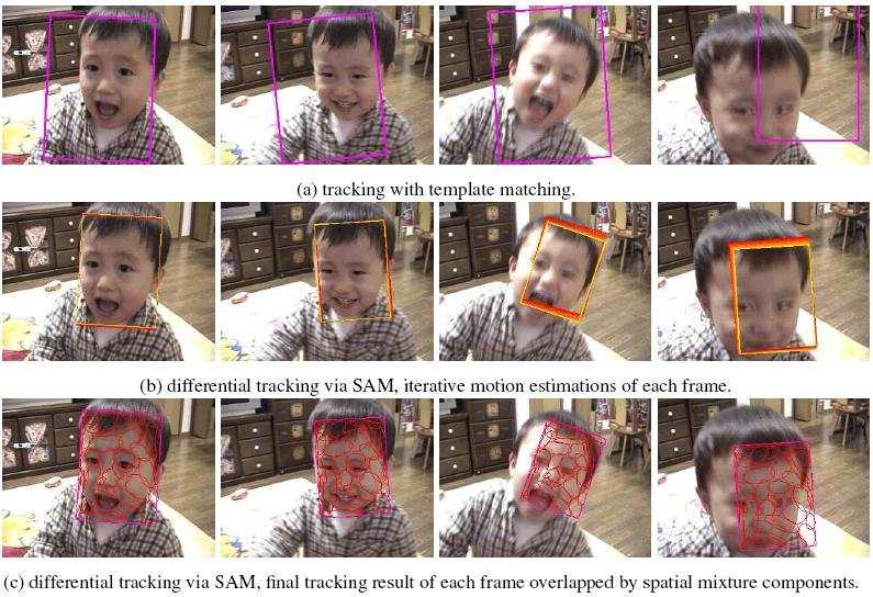
23 Spatial-appearance model (SAM) 23/52

24 Outline Optical Flow Beyond Basic Optical Flow Considering Lighting Variations Considering Appearance Variations Considering Spatial-Appearance Variations Kernel-based Tracking Basic kernel-based tracking Multiple kernel tracking Context Flow 24/52

25 Representation The target is represented by a feature histogram q = [q 1, q 2,...,q m ] T R m, where q u = 1 C n K(s i x)δ(b(s i ), u) i=1 its matrix form q(x) = U T K(x) δ(b(s 1 ),u 1 )... δ(b(s 1 ),u m ) U =... R n m, K = 1 K(s 1 x) C. R n. δ(b(s n ),u 1 )... δ(b(s n ),u m ) K(s n x) Kernel profile: K(x) = k( x 2 ) denote by g(x) = k (x) 25/52

26 Formulation The target is initially at x to find the optimal motion x by mino(q,p(x + x)) x where q is the target model, and p is the image observation choices of O(, ) Bhattachayya coefficient O B ( x) = q, p(x + x) = q T p(x + x). Matusita metric O M ( x) = q p(x + x) 2. 26/52

27 Mean-shift tracking 6 O B = m pu (x + x)q u u=1 first order approximation O B ( x) = 1 2 where w i = m u=1 m u=1 pu (x)q u + 1 2C n i=1 w i K( x + x s i 2 ) h qu δ(b(s i ), u) p u (x) is the weight for s i CVPR 00 6 D. Comaniciu, V. Ramesh and P. Meer, Real-Time Tracking of Non-Rigid Objects using Mean Shift, 27/52

28 Mean-shift tracking So, we have min O B( x) = max x x n i=1 w i K( x + x s i 2 ) h The solution is an iterative mean-shift procedure x n i=1 n i=1 s i w i g( x s i 2 ) h w i g( x s i 2 ) h 28/52

29 SSD kernel-based tracking 7 let s use O M ( x) = q p(x + x) 2 Linearization where p(x + x) p(x) d(p(x)) 1 2 U T J k (x) x d(p(x)) = diag(p 1 (x),...,p m (x)) J k = [ c K(s 1 x) ] K K u v =. c K(s n x) 7 G. Hager, M. Dewan and C. Stewart, Multiple Kernel Tracking with SSD, CVPR 04 29/52

30 SSD kernel-based tracking So the objective function is O M ( x) = q p(x) 1 2 d(p(x)) 1 2 U T J k (x) x 2 Denote M(x) = 1 2 d(p(x)) 1 2U T J k (x) we have a linear system M x = q p(x) the solution is clear x = M ( q p(x)) 30/52

31 Singularities It is clear that M is in the form of d 1 x M =. d m x d 1 y. d m y where [ d j x d j y ] = 1 2 (s j i p x)g s j i x 2 j h i which is the center of mass for feature j. {[ ] } If dx j dy j, j = 1,...,m are linearly dependent, then rank(m) = 1 and the solution is not unique. 31/52

32 Optimal Kernel Placement 8 Different image regions have different properties. Some of them are singular, and some are far from singular. How can we find those that are far from singular? Checking the property of M. The Schatten 1-norm: A S = σ i The S-norm condition number κ S (A) = ( σ i ) 2 / σ i we can compute in a closed form κ S (M T M) = (M T M) S (M T M) S = exhaustive search v.s. gradient-based search ( (d j x) 2 + (d j y) 2 ) 2 (d j x ) 2 (d j y) 2 ( (d j xd j y)) 2 8 Zhimin Fan, Ming Yang, Ying Wu, Gang Hua and Ting Yu, Efficient Optimal Kernel Placement for Reliable Visual Tracking, CVPR 06 32/52

33 Optimal Kernel Placement 33/52

34 Kernel Concatenation Concatenate multiple kernels to increase the dimensionality of measurement the same as using more features a set of K kernels p i (x) = U T K i (x) stacking histograms into p and q. the objective function is min x K q p i (x + x) 2 i=1 easy to see the solution where M = 1 2 d(p) 1 2 M x = q p i (x) U T... U T J K1. J Kw 34/52

35 Kernel Combination Aggregating histograms to produce new features K K q = U T K i, p = U T K i (c). i=1 i=1 The objective function is min K q K p i (x + x) 2 x i=1 i=1 The corresponding linear system is: K q i K p i (x) = M x, i=1 i=1 where M = 1 K 2 d(p) 1 2 U T J Ki = K i=1 i=1 M i 35/52

36 Collaborative Multiple Kernels 9 x 1 Relaxed motion representation x =. x k Consider a structural constrain Objective function O(x 1,...,x k ) = Ω(x 1,...,x k ) = 0 k q i p i (x i ) 2 + γ Ω(x 1,...,x k ) 2 i=1 This is equivalent to a linear system { l = G x + ω1 y = M x + ω 2, 9 Zhimin Fan, Ying Wu and Ming Yang, Multiple Collaborative Kernel Tracking, CVPR 05 36/52

37 Collaborative Multiple Kernels where q1 M p(x 1 ) M y =. qk, M = , p(x k ) M k ] Ω Ω G = x 2 x k, l = Ω(x 1,x 2,...,x k ) [ Ω x 1 We have ([ ]) M rank γg rank(m) it enhances the motion observability 37/52

38 An Example special case: x 1 = x 2 =... = x k, and γ is chosen as the optimal Lagrangian multiplier, then I I I I G =......, and l = 0. I I we have rank(g) = (k 1) dim(x 1 ). E.g., supposing k = 10 and dim(x 1 ) = 2, this implies that the motion resides in a 2-D manifold in R 20. Thus, as long as rank(m) dim(x 1 ), all the motion parameters are observable, or can be uniquely determined. It is be easily satisfied if any of the xi is observable through its kernel, there are a number of dim(x1 ) motion parameters that are observable through multiple kernels. 38/52

39 Solution and Collaboration The solution x = (M T M + γg T G) 1 (M T y + γg T l). A more efficient solution x = (I D)(M T M) 1 (M T y + γg T l), where D = γ(m T M) 1 G T (γg(m T M) 1 G T + I) 1 G Notice that x u = (M T M) 1 M T y = M y, is the solution to the independent kernels, and x = (I D) x u + z(x) The collaboration through a fixed-point recursion x k+1 (I D k )[M( x k )] y k + z k, 39/52

40 MKL for scale 10 Determining the scale of the target is an important issue It is related to the scale of the kernel Basic idea: using mean-shift in the spatial-scale space (x, σ) Algorithm: alternating a spatial mean-shift and a scale one 1. initial states (x 0,σ 0 ); 2. fix σ 0, perform a 2-D spatial mean-shift to obtain x ; 3. fix x, perform a 1-D scale mean-shift to obtain σ ; 4. repeat 2 and 3 until convergence. 10 Robert Collins, Mean-shift Blob Tracking through Scale Space, CVPR 03 40/52

41 Outline Optical Flow Beyond Basic Optical Flow Considering Lighting Variations Considering Appearance Variations Considering Spatial-Appearance Variations Kernel-based Tracking Basic kernel-based tracking Multiple kernel tracking Context Flow 41/52

42 Distraction and Matching Ambiguity Spatial context can reduce matching ambiguity Questions: Modeling context for motion analysis? Methods resilient to local variations? 42/52

43 Spatial Context (for object recognition) Structure-stiff (e.g., template and filters) Structure-flexible random fields deformable templates shape context, AutoContext Structure-free bag-of-words or bag-of-features 43/52

44 Modeling Spatial Context Location x is associated with features f(x) feature class {ω 1,...,ω N } individual context: C i = {y f(y) ω i,y Ω(x)}, N total context: C = C i. i=1 context representation: p(ω i x) p(x ω i )p(ω i ) 44/52

45 Contextual Maps 45/52

46 Brightness Constancy Context Constancy 11 Context constancy p(ω i x + x, t + t, C) = p(ω i x, t, C) The motion x shall not change the context More flexible than constant brightness insensitive to lighting insensitive to local deformation Let s impose a small motion assumption Ying Wu and Jialue Fan, Contextual Flow, CVPR 09 46/52

47 A Differential Form T x p(ω i x, t) }{{} x + t p(ω i x, t) }{{} t = 0 contextual gradient contextual frame difference Contextual frame difference is approximated by p(ω i x, t + t) p(ω i x, t) Contextual gradient (details follow) { x p(ω i x) = x p(ω i ) p(x ω } i) p(x) = 1 [ ] c p(ω i x) µ i (x) µ 0 (x) 47/52

48 Context Gradient Conditional Shift µ i (x) = E{(y x) y ω i } = 1 Z i (x) After simple manipulation Total shift µ i (x) = c xp(x ω i ) p(x ω i ) µ 0 (x) = E{(y x) y Ω} = c xp(x) p(x) Ω (y x)p(y ω i )dy so we have x p(ω i x) = 1 [ ] c p(ω i x) µ i (x) µ 0 (x) 48/52

49 Illustration: Contextual Gradient 49/52

50 Context Flow Constraint It is easy to see: [ ] [ T p(ωi x, t + 1) µ i (x) µ 0 (x) x + c }{{} p(ω i x, t) µ i (x) ] 1 } {{ } b i = 0 µ i (x) is the centered shift b i is the change of context ratio Contextual flow constraint µ i (x) T x b i = 0 50/52

51 Local Contextual System Each context gives a constrain weighted by W i (x) = p(ω i x, t), and W(x) = diag[w 1 (x),...,w N (x)] Denote by U r (x) = [ µ 1 (x),..., µ N (x)] T, br (x) = [b 1, b 2...,b N ] T, U(x) = W(x)U r (x), b(x) = W(x)b r (x) we have a linear contextual system U(x) x = b(x), or simply U x = b 51/52

52 Extended Lucas-Kanade Method If U is rank deficient, we have an aperture problem as well Considering the nearby locations X = {x 1,...,x m } each of which is associated with a contextual system U i (x i ) x i = b(x i ), or simply U i x i = b i where x i is the motion for location x i. If they share the same motion, i.e., x i = x, then Extended Lucas-Kanade method U 1 b 1... x = U c x =... U m b m 52/52