Predictive Modeling Using Logistic Regression Step-by-Step Instructions

Transcription

1 Predictive Modeling Using Logistic Regression Step-by-Step Instructions This document is accompanied by the following Excel Template IntegrityM Predictive Modeling Using Logistic Regression in Excel Template.xlsx Two datasets are used to run predictive modeling based on prior information: Step 1: Training dataset - This dataset includes both historical and current data with distinction of the outcomes coded 1 for Yes and 0 for No. Steps 1 to 7 use the dataset to assess the relative importance of indicators/variables to the outcome (Weights) and to determine the strength of their association with the outcome (P-values). Scoring dataset - new data on individuals/entities/ids used to compute the probability of outcome. Input your analytical file; in our example, we downloaded data from the Office of Inspector General List of Excluded Individuals and Entities (LEIE) and from the Centers for Medicare and Medicaid Services (CMS) Public Use File (PUF). Columns A to G of the spreadsheet Predictive Model display the data. The analytical file includes columns A to G. Column A displays the provider identifier and columns B to G show summary information on the variables per provider inputted to the analysis, including the response variable informing if the provider was excluded or not (coded 1 or 0 respectively). The working dataset consists of information stored in cells B2 to G92. Steps 2 and 3: Copy values from column H (RANDBETWEEN Values) to column I (P (E)) this is necessary because of the volatile nature of the formula in column H, which will values changed every time the spreadsheet is refreshed. The rest of the columns in Step 3 will be computed automatically by the formulas embedded in them (Column J (Odds Ratio), Colum K (If Odds Ratio < 0.1 set it to 0.1) and Column L (Log (Odds Ratio)) The Excel function RANDBETWEEN assigns random probability numbers to the providers according to their original classification ( 1 or 0 ) - drawing from the range 0.50 to 0.99 for providers coded 1 (excluded) and from the range 0.01 to 0.49 for providers coded 0 (active in the health care program) Note that the RANDBETWEEN function requires as input values integers (numbers) that define the bottom and the top values from which a random number will be drawn. The values will be stored in column H, RANDBETWEEN Values. The assigned values need to be transformed to probability numbers by dividing the function output number by 100 according to the provider exclusion status and the following Excel operation: for excluded providers, =RANDBERWEEN(50, 99)/100; for non-excluded (active) providers, =RANDBERWEEN(1, 49)/100;

2 Step 4: Step 4.1: o Run the Linear Regression Model by using the Data Analysis tool of Excel as shown in the screenshot below to obtain the Initial weights (coefficients) of the variables/indicators (in our example, 5 variables). The regression input Y Range (response variable) is the Log(Odds), column L; and the five indicators in Input X Range are all values in PMT per Bene, Services per Bene, Average Age of Beneficiaries, Beneficiary cc diab percent and Average HCC Risk Score of Beneficiary columns C to G. The Regression Model results will generate a new tab labeled in our example Step 4 - Reg Initial Values. Step 4.2: o Copy the coefficients (weights) in column B from the regression model output to the Coefficients Table (in our example, the table includes cells T3 to T8 in column T of the spreadsheet Predictive Model ).

3 Step 5: Update the formula in Column N (variable labeled L) if you have more or less than the 5 variables that we have in our example. This formula includes the initial values of the weights from the Coefficients Table (Column T in our example) multiplied by the corresponding indicators (columns C to G in our example). Changes in the set of summation terms in the cases of 4 or 6 variables would be 4 variables, formula =T$3 + T$4*C4 + T$5*D4 + T$6*E4 + T$7*F4 + T$8*G4 6 variables, formula = T$3 + T$4*C4 + T$5*D4 + T$6*E4 + T$7*F4 + T$8*G4+T$9*H4

4 Note: the mathematical constant e (= in cell T10 in our example) is required to compute the results in column O (labeled el = "e to power L"). The values of column P (P(X) = el/(1 + el)) and column Q (Y*ln[P(X)] + (1 Y)*ln[1 P(X)]) will be updated automatically (where Y = 1 for excluded providers and Y = 0 for active providers) by the embedded formulas. Step 6: Step 6.1: o Update the summation of the Log (Maximum Likelihood) if you have more rows than our example: If you have 100 rows in your data rather than the 90 rows of our example, change the formula from =SUM(Q3:Q92) to =SUM(Q3:Q102) Step 6.2: o Run the Excel Solver tool to obtain the set of final weights that define the relative importance of the indicators/variables to the outcome. The Excel Solver will work on the set of initial weights (previously generated by the logistic regression) to update the Coefficients Table with a set of final weights that maximizes the likelihood of obtaining the data (outcome variable and indicators) actually observed. The Excel Solver will generate an output tab that is labeled Step 6 - Solver Final Values in our example.

5 Note: the signs of the regression coefficients indicate whether additional units of the associated variables increase (positive sign) or decrease (negative sign) the probability that the analyzed provider will reach the target outcome (joining the OIG Exclusion List in this example). For example, the average payment per beneficiary (positively associated with the probability of exclusion) for excluded providers $ as opposed to $ for non-excluded (active) providers; on the other hand, the average risk score per beneficiary (negatively associated with the probability of exclusion) is for excluded providers in contrast with for non-excluded providers. Step 7: Steps 7.1 to 7.7 determine the strength of the association (p-values) of each Indicator/variable (explanatory variable) with the outcome variable (the probability of being excluded from the Medicare program in our example) by estimating the covariance matrix of the model. Step 7.1: o Construct an Excel table having a row per provider and a column per variable without including the provider identifier; add to the table a column of 1s (intercept). In our example the table includes columns A to F of the spreadsheet Step 7 - Covariance Matrix (intercept plus five variables - PMT per Bene, Services per Bene, Average Age of Beneficiaries, Beneficiary cc diab percent and Average HCC Risk Score of Beneficiary ). Step 7.2:

6 o Copy values from column P (labeled P(X) = el/ (1 + el)) from tab Predictive Model to column G (labeled P(X) = el/ (1 + el)) in tab Step 7 - Covariance Matrix. Values in column H (labeled (1 - P(X))) and column I (labeled P(X)*(1 - P(X))) will be updated automatically by the embedded formulas. Note: From steps 7.3 to 7.6, remember to highlight the destination cells (range of cells) BEFORE completing the formula with Shift-Control-Enter Note: The destination of the transpose operation needs to be highlighted (cells B97 to CM102 in our example) before the re-scaled table (cells K4 to P93) is transposed. Operations with matrices (tables) in Excel are explained in Notes on Matrix Operations in Excel by Ronald Larsen, Step 7.3: o Multiply every row of the table created in step 7.1 (cells A4 to G93 in our example) by the values in column I (P(X)*(1 - P(X))), to generate a re-scaled table stored in cells K4 to P93. This multiplication is accomplished in row 4 by the Excel function =I4*(A4:F4), which is copied and pasted to all rows from 5 to 93. Note: Remember to highlight the destination cells (range of cells) BEFORE completing the formula with Shift-Control-Enter Step 7.4: o Transpose the re-scaled table stored in cells K4 to P93 using the Excel matrix function TRANSPOSE(re-scaled table) to generate the transposed table stored in cells B97 to CM102 in our example. Note: Remember to highlight the destination cells (range of cells) BEFORE completing the formula with Shift-Control-Enter

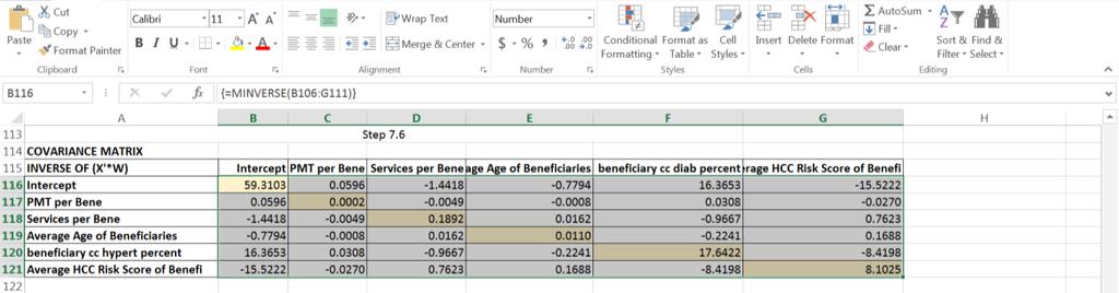
7 Step 7.5: o Multiply the transpose of the re-scaled table, computed in the previous step and stored in cells B97 to CM102, by the original (not re-scaled) table stored in cells A4 to F93 using the Excel matrix function MMULT(transpose of the re-scaled table, original table) to create a product table stored in cells B106 to G111. Note: Remember to highlight the destination cells (range of cells) BEFORE completing the formula with Shift-Control-Enter. Step 7.6: Compute the inverse of the table created in the step 7.5 using the Excel matrix function MINVERSE(product table) to create the covariance matrix, which is stored in cells B116 to G121. The highlighted main diagonal values as shown below are the variances of the variables to be used in Step 7.7. Note: Remember to highlight the destination cells (range of cells) BEFORE completing the formula with Shift-Control-Enter

8

9 Step 7.7: Copy the coefficients (weights) computed by the Excel Solver from the cells T3 to T8 (in our example) from tab Predictive Model to the cells B126 to B131 of tab Step 7 - Covariance Matrix. The final weights are also found in the Excel Solver output tab. Copy the variances of the variables from the main diagonal of the covariance matrix cells B116, C117, D118, E119, F120 and G121 - to cells C126 to C131 in column C of tab Step 7 - Covariance Matrix. Note: the next steps will calculate new values automatically using the weights and variances inputted in the previous steps. The standard deviations are computed using the Excel function SQRT(variance) applied to values in cells C126 to C131 and store the results in cells D126 to D131 in our example. The Wald Chi-square statistic for each variable is computed as the squared value of the ratio (coefficient/standard deviation) and stored it in cells E126 to 131 under the label Wald in our example. The strength of the association p-value is computed using the Excel function CHISQ.DIST.RT(Wald,1), where the second input to the function - the number 1 - is the number of degrees of freedom in this case. The p-values are stored in cells F126 to F131. Note: The P-value of each variable assesses the strength of the association between the variable and the outcome. The lower the p-value the stronger the association between variables. The standard rule is to consider p-values <= 5% (0.05) as indicative of statistically significant association. In our example, all variables were found to be strongly associated with the outcome. The screenshot below reproduces the results of the predictive model analysis using the same data but implemented with the statistical package SAS, which generates exactly the same results as the ones obtained using Excel. Step 8:

10 Steps 8 to 10 use a new dataset of active (unclassified as excluded) providers to score their probability of joining the OIG Exclusion List Step 8.1: o Input your Scoring dataset - our example used a sample of 100 non-excluded providers. The dataset included the 5 indicators and used the final weights to score their probability of being excluded. The final weights are inputted in columns K to P in our example. Step 8.2: o The formulas embedded in columns G to I will generate values based on the data inputted. Note: the value of the mathematical constant e (= , copied to the cell N3) is used to compute values in column G (labeled L). The probabilities of exclusion P(X) of provider in row 2 are generated by using the formula =H2/(1 + H2), where the values of H2 are computed in the previous operation.