Designing Information Devices and Systems II Fall 2015 Note 22

Transcription

1 EE 16B Designing Information Devices and Systems II Fall 2015 Note 22 Notes taken by John Noonan (11/12) Graphing of the State Solutions Open loop x(k + 1) = Ax(k) + Bu(k) y(k) = Cx(k) Closed loop x(k + 1) = (A BKC)x(k) + BKr(k) y(k) = Cx(k) In fact, people have called feedback, "automatic control" because one is automatically controlling the actuators to the system through this feedback loop. Using our open loop terms (since this holds for both the open loop and closed loop system... we derived that: u(0) u(1) x(k) = A k x 0 + [A k 1 BA k 2. B...B].. u(k 1) EE 16B, Fall 2015, Note 22 1

2 These represent columns of the matrix. If there is just a single input to the system then the matrix on the left will be a single column but if there are multiple inputs, the matrix will expand in the columns. - Last time we looked at different cases: Case A: Zero Input u(0) = u(1) =... = u(k 1) = 0 and we asked, "how does x(k) - the state trajectory / solution look like for different patterns of eigenvalues of the matrix A. Case 1: A is diagonalizable. This means that A has n linearly independent eigenvectors, which further implies that we can use them to form a basis for our state space. In particular, we can write our initial state x 0 as a linear combination of sigmas and v s (the eigenvectors). x 0 = σ 1 v 1 + σ 2 v σ n v n. The eigenvectors can be complex, so if there is a complex eigenvector, it has to appear with its complex conjugate pair, so the imaginary parts cancel out. Example: n = 2 (however this is general, so it applies to any finite n) x 0 = σ 1 v 1 + σ 2 v 2 We do this because there is a particularly simple form to the solution: x(k) = A k (σ 1 v 1 + σ 2 v 2 ) Since the sigmas are scalars, we can bring them outside. x(k) = σ 1 λ k 1 v 1 + σ 2 λ k 2 v 2 Last time we focused on what happened when our eigenvalues are all real. The unit circle is important because, as we see from the equation we just wrote, if these eigenvalues have magnitude greater than 1, the solution x(k) will blow up as k gets large. If the magnitude is less than 1, the solution will decay. So, it is important to think about the concept of stability with regard to the magnitude of the eigenvalues. Back to the unit circle, even if the eigenvalues are inside the unit circle or on the unit circle, what are the type of patterns will we see in the response? We looked at combinations of eigenvalues when the eigenvalues were repeated at the same spot. When the eigenvalues were on the negative real axis, we saw this periodic or oscillatory behavior in the solutions. And for the eigenvalues that were on the positive real axis, we saw a constant decay as long as the magnitudes were strictly less than 1. And if the eigenvalues were on the unit circle, we saw that the solution was the same as the initial condition. Let s consider case f) where the eigenvalues appear in complex conjugate pairs. Before we proceed, what happens when the eigenvalue is 1 (the other eigenvalue is less than 1) - in relation to the Page Rank problem - is that it converges to that first eigenvector. EE 16B, Fall 2015, Note 22 2

3 Revisit of cases of real eigenvalues A is diagonalizable and n = 2 Case (b): λ 1,λ 2 R λ 1 < 1, λ 2 < 1 λ 1,λ 2 > 0. A is in general diagonalizable, not diagonal. Remark: If A is diagonal, then the eigenvectors v 1 and v 2 will be the x 1 and x 2 axes. In general, when A is diagonalizable, they are not the x 1 and x 2 axes, but we know that they are linearly independent, so they span R 2 Now let s "graph x(k)"... meaning, let s plot x 2 (k) vs x 1 (k). We know that the initial condition is a linear combination of the eigenvectors. Since v 1 and v 2 span R 2, x 0 could be anywhere. Now, we need to determine the solution as k goes to infinity. Recall: (b) Now, we re starting off with an initial condition where both coordinates are positive and equal to each other. The magnitude of the eigenvalues was 0.5 which tells us that whatever the initial condition is, we re going to see that the solution is: We only see the trajectory go in. If we start on v 1, we will stay on v 1. We will still converge to 0, but on v 1. EE 16B, Fall 2015, Note 22 3

4 If we start on v 2, we will converge to 0 and stay on v 2. If we start off the eigenvectors, we stay on a linear combination of the eigenvectors in a "star burst" pattern. Note: we are not plotting with respect to time. Case 2: λ 1,λ 2 R λ 1, λ 2 < 1 λ 1,λ 2 > 0. λ 1 = 0.1,λ 2 = 0.9 The eigenvector v 1 is the eigenvector corresponding to λ 1 so it is much closer in to the zero than v 2. Now, consider the initial point shown in green. The trajectory will converge towards v 2 as it goes toward the origin. If it starts on v 1, it will stay on v 1, and if starts on v 2, it will stay on v 2, but off of v 1, it will tend to converge to v 2. How they curve in depends on the relative magnitude of the eigenvalues. In general, we care about stability and the shape of the solution. Remember: x 0 = σ 1 v 1 + σ 2 v 2 if x 0 is on v 1 ; x 0 = σ 1 v 1. EE 16B, Fall 2015, Note 22 4

5 Also, note that we cannot have solutions crossing in the plane. We will get a unique solution for each start point. Example: If we start on the positive real axis (shown in green), we will get the trajectory shown (also in green) from that point converging towards v 1 to the origin. Case 3: λ 1, λ 2 < 1 λ 1 > 0 > λ 2 EE 16B, Fall 2015, Note 22 5

6 If we start on v 1, we will stay on v 1 and converge to 0. If we start on v 2, we will stay on v 2, but we will jump back and forth between positive points and negative points on the v 2 line. The convergence to 0 will also happen faster since the eigenvalue is close to 0. We get the following trajectories: The geometry of the convergence depends on the eigenvectors, and it depends on the relative magnitudes of the eigenvalues with respect to the eigenvectors. Now, let s look at the "overshoot" case: We want it to step up and stay at 1, but we get oscillatory overshoot behavior. What does this say about the eigenvalue associated to x 1 (say, it s a diagonal system)? This is indicative of the eigenvalue being on the negative real axis. It is converging to something that is not zero, where it s magnitude has to be between 0 and Case 4: λ 1,λ 2 R λ 1,λ 2 > 0. λ 1 > 1 > λ 2. Again, if we start on an eigenvector, we will stay on an eigenvector, but now because the eigenvalue is EE 16B, Fall 2015, Note 22 6

7 greater than 1, the trajectory will go off the eigenvector, shown in the diagram. If we start at a point very close to v 1, the trajectory will take off in the v 1 direction. If we start at a point very close to v 2, the trajectory will start to go in the v 2 direction, but then turn around and take off in the v 1 direction. Remember, to be unstable, there needs to be an eigenvalue which is greater than 1. Also, if one of the eigenvalues is greater than 1 (which means that it is not stable) but the other eigenvalue is less than 1, then we get something called a "saddle condition," and the trajectory looks like the following: The reason it is called a "saddle" is because if we consider a saddle for a horse, and we roll a marble down the center line of the saddle, and it is perfect without noise, it s just going to converge at the center point. This EE 16B, Fall 2015, Note 22 7

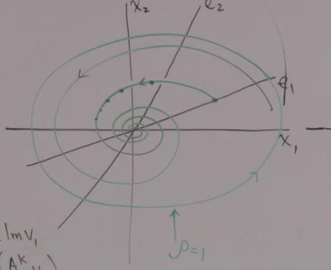
8 corresponds to our stable eigenvector. But as soon as we start at a point just off of that stable eigenvector, the trajectories should diverge away and go off to infinity. (Also, based on what we ve drawn, the eigenvalue of the stable eigenvector would be negative.) - Example: The case when the eigenvalues are complex. As we discussed, they have to appear in complex conjugate pairs. Case 5: λ 1,λ 2 C λ 1 = λ 2. v 1 = e 1 + je 2 v 2 = e 1 je 2 λ 1 = ρe jθ λ 2 = ρe jθ x 0 = αv 1 + ᾱv 2, α = α 1 + jα 2. So, x 0 = α 1 e 1 + α 2 e 2, where e 1 corresponds to the real part and e 2 corresponds to the imaginary part. Now, we no longer have the property that if we start on e 1, we will stay on e 1. EE 16B, Fall 2015, Note 22 8

9 x 0 = α 1 e 1 + α 2 e 2 = α 1 Re(v 1 ) + α 2 Im(v 1 ) x(k) = A k x 0 = α 1 Re(A k v 1 ) + α 2 Im(A k v 1 ) = α 1 Re(λ k v 1 ) + α 2 Im(λ k v 1 ) x(k) = α 1 Re(ρ k (cos(θk) + jsin(θk)(e 1 + je 2 )) + α 2 Im(ρ k (cos(θk) + jsin(θk)(e 1 + je 2 )) x(k) = α 1 ρ k cos(θk)e 1 + α 2 ρ k sin(θk)e 1 α 1 ρ k sin(θk)e 2 + α 2 ρ k cos(θk)e 2 In general, the solution will oscillate around the vectors v 1 and v 2. The magnitude of the trajectory will depend on ρ, but the oscillation will depend on θ. In particular, at each time k, we will pick up a new point, and the frequency of that point depends on θk. So, we start off at some initial point. Then, the next point will have magnitude which is defined by the magnitude ρ and a phase which is defined by the phase of the eigenvalue times the particular value of k. If we have complex eigenvalue pairs which have magnitude greater than 1, then the spirals will basically go off to infinity. The trajectory will spiral out with growing and growing radius because of the dependence on ρ k - that magnitude will get greater and greater as k gets large. The complex component of the eigenvalues is contributing a phase which gives an oscillatory component in the underlying trajectory of the solution. Now, if ρ is 1, meaning the eigenvalues are on the unit circle, then the trajectory will be an ellipse. EE 16B, Fall 2015, Note 22 9

10 We give names to these trajectories. When it is spiraling in, it is called a "focus." When it is circling about in an oscillatory behavior, we call that a "center behavior." And the real cases done previously are called "nodes." EE 16B, Fall 2015, Note 22 10

11 EE 16B, Fall 2015, Note 22 11