TMA 4265 Stochastic Processes Semester project, fall 2014 Student number and

Transcription

1 TMA 4265 Stochastic Processes Semester project, fall 2014 Student number and Exercise 1 We shall study a discrete Markov chain (MC) {X n } n=0 with state space S = {0, 1, 2, 3, 4, 5, 6}. The transition probability matrix of the MC is P = a) Equivalence classes The chain has three equivalence classes {0, 1}, {2, 3} and {4, 5, 6}. Whether they are recurrent or transient can be determined from figure 1. The circles denote states in the state space and there are arrows between all states with transition probability greater than 0. {0, 1} is transient because it is possible to leave the class, and once having left, it is impossible to go back. Hence the states 0 and 1 will only be visited a finite number of times. The period of a state i is the greatest common divisor of all integers n 1 for which P n ii > 0. P n ii > 0 is the probability of returning to state i in n steps. P n 00 > 0 for all n 1. Hence the equivalence class {0, 1} is aperiodic. {2, 3} is recurrent because once you enter the class, you cannot leave. Hence the states 2 and 3 will be visited infinitely often. P n 33 > 0 for all n 1. Therefore the equivalence class {2, 3} is aperiodic. {4, 5, 6} is recurrent because once you enter the class, you cannot leave. Hence the states 4, 5 and 6 will be visited infinitely often. P n 44 > 0 for n = 3, 6, 9,... Thus it takes three steps to go from state four and return to state four. This is also the case for state 5 and 6. Therefore the equivalence class {4, 5, 6} has period 3. 1b) Stationary probabilities Q = X X X X X X X X X X X X X X X 1

2 Figure 1: State space and possible transitions between states in the MC. Stationary probabilities are the probability of being in state j at any time n. A Markov chain can have several stationary distributions. If the MC is irreducible and ergodic, there exists a limiting distribution, π j = lim P ij, n j 0 because there is only one n stationary distribution. This means that a limiting distribution is always a stationary distribution, but the converse is not necessarily true. The elements of lim n P(n) which do not exists are marked by an X in Q, and those that exist are marked by a 0 if the limit is 0 and a if the limit exists but is not zero. The elements lim n P n ij, i = 0, 1, 4, 5, 6, j = 4, 5, 6 do not have a limit because the equivalence class {4, 5, 6} is not aperiodic. The elements lim P ij, n i = 0, 1, 2, 3, 4, 5, 6, j = 0, 1 do have a limit, which is 0. This n is because the equivalence class {0, 1} is transient and when you leave the class, you cannot reenter. The probability of staying in {0, 1} is less than 1, therefore Pii n, i = 1, 2 approaches 0 as n. The elements lim P ij, n i = 2, 3, j = 4, 5, 6 have a limit, which is 0, because the equivalence class {2, 3} is recurrent, hence you cannot enter {4, 5, 6}, given initial state X 0 = n 2 or X 0 = 3. The elements lim P ij, n i = 4, 5, 6, j = 2, 3 also have this limit because the n equivalence class {4, 5, 6} is recurrent. The elements lim P ij, n i = 0, 1, 2, 3, j = 2, 3 have a limit not equal to zero. This is n because the equivalence class {2, 3} is irreducible and ergodic. Hence there exists only one stationary distribution which is the limiting distribution. 2

3 1c) Expected proportion of time in different states We shall determine the expected proportion of time that the chain spends in the different states, depending on the initial state. Figure 2: The expected proportion of time that the chain spends in the different states, depending on the initial state. The element (.) ij in the matrix in figure 2 denotes the proportion of time spent in state j given that the MC starts in state i. As an example, u 0 is the proportion of time spent in state 2 given that the initial state is 0. 3

4 Figure 3: Calculated values of π i, i = 2,3,4,5,6, in figure 2. 4

5 Figure 4: Calculated values of u 0 and u 1 in figure 2. 5

6 Figure 5: Calculated values of v 0 and v 1 in figure 2. 6

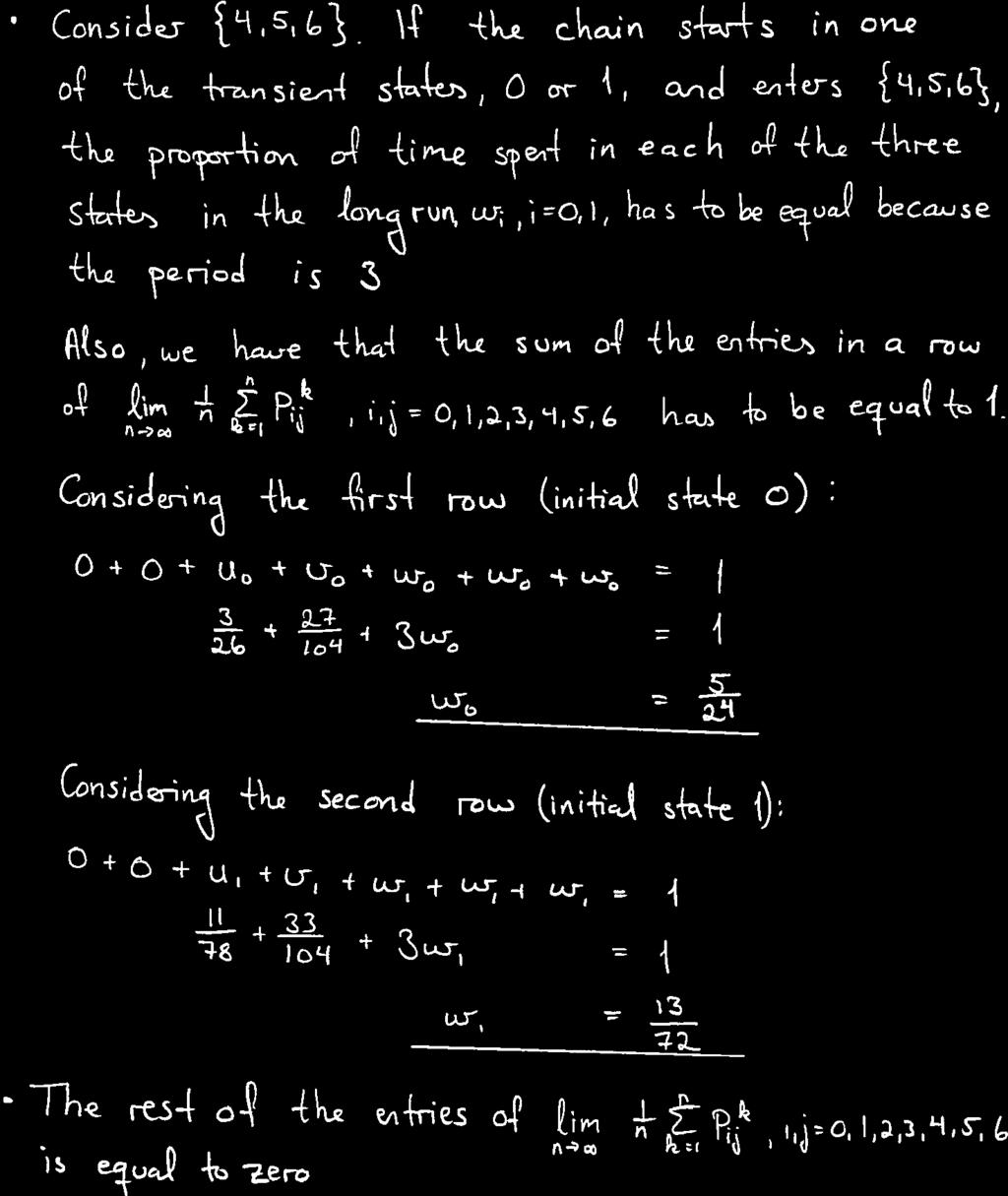
7 Figure 6: Calculated values of w 0 and w 1 in figure 2. 7

8 The calculations in figure 3, 4, 5 and 6 give 1 lim n n n P (k) = k=1 1d) Simulations of MC By calculating the matrix 1 n n k=1 P(k) numerically for large n, we get approximately the same matrix as calculated above. The probability that the chain ends up in state 0 or 1, given initial state X 0 = 0, 1 is not exactly 0, but as n increases, these entries approaches 0, as expected. The other entries of 1 n n k=1 P(k) which are zero, are identically zero for all n, because these steps have a probability identical to 0. A script written in R which does this simulation is included in the section R-code on page 13. In the same section, there is also a script in which a Markov chain is simulated times, given initial state X 0 = 0. We obtain ( ). These entries are the approximate proportion of time the chain spends in each state, 1 n given initial state X 0 = 0. These proportions approach the top row of lim P (k). n n k=1 This verifies the results in exercise 1c. 8

9 Exercise 2 We are interested in finding: i) The distribution of the life time of the mouse. ii) Probability that mouse and cat are never in neighbouring rooms 2a) Discrete time Markov Chain Let X n denote the smallest number of doors that separate the mouse and the cat at time point n, n = 0, 1, 2,. The state space for X n is S = {0, 1, 2}. If X n = 0, the mouse is in the same room as the cat and gets eaten. The number of doors X n+1 is only dependent on X n because both the cat and the mouse move once at every time step n. Therefore X n can be modelled using a Markov Chain {X n } n=0. The transition matrix of the MC is P = The probabilities for how the cat and the mouse act are given. At all time steps, P (cat moves) and P (mouse moves) are both 0.45 and P (cat stays) and P (mouse stays) are both 0.1. P 00 = 1 because the cat and the mouse must be in the same room when the cat has eaten the mouse. State 0 is an absorbing state. Consequently, the other elements in the first row are 0. When starting in neighbouring rooms, there are two possibilities that they will end up in the same room. Either the mouse moves and the cat stays or the cat moves and the mouse stays. Because they move independently of each other, the resulting probability is P 10 = P (cat moves) P (mouse stays) + P (cat stays) P (mouse moves). The same logic and numbers apply for the case P 12. There are four ways for them to end up in neighbouring rooms after having moved. Either they both move clockwise, anti-clockwise, one in each direction or they interchange rooms. A final possibility is that none of them move. P 11 = 4 P (cat moves) P (mouse moves) + P (cat stays) P (mouse stays) When starting two doors apart, there are two possibilities that they will end up in the same room. In either way, one of them will move clockwise and one will move anticlockwise. P 20 = 2 P (mouse moves) P (cat moves). The possibility that they end up one door apart is the sum of possibilities: one of them stays and the other one moves clockwise or anti-clockwise. P 21 = 2 P (mouse moves) P (cat stays) + 2 P (mouse stays) P (cat moves). 9

10 There are three ways for them to end up two doors apart. Either they both move in different directions or they both stay. P 22 = 2 P (cat moves) P (mouse moves) + P (cat stays) P (mouse stays). In order to find the equivalence classes of the state space, we examine how the states communicate. Figure 7 provides an overview of accessibility between states. The circles denote states in the state space and there are arrows between all states with transition probability greater than 0. Starting in state 1, it is possible to access both states 2 and 0. Starting in state 2, it is possible to access both states 1 and 0. It is, however, not possible to reach states 1 or 2 when starting in state 0. If the MC starts in 1, the expected number of times 1 is visited is finite because the MC at one point will reach the absorbing state 0. Therefore {1, 2} is a transient equivalence class. When the MC reaches state 0, it can never leave. Therefore {0} is a positive recurrent equivalence class Figure 7: Statespace and possible ways to move between states 2b) Expected life time of a mouse The expected life time of the mouse is finite. We know that at some point the cat will be in the same room as the mouse, which is an absorbing state. To find the mean time the MC spends in transient states, before it gets to state 0, we calculate the number of visits in each transient state. Let s ij be the expected number of visits in a state j when the MC starts in state i. Then, in matrix notation, S = (I P T ) 1. Here, I is the identity matrix and P T is the transient part of P, i.e. transitions from either states 1 or 2 to states 1 or 2. S is the matrix with elements s ij. S = ( ) In order to calculate the mean time spent in transient states when the MC starts in state 2, we sum all row entries in s 2j, j = 1, 2. When the cat and the mouse start two 10

11 doors apart, the mouse is expected to live time steps. So the mouse is expected to survive 4 hours. Simulations of the MC yields similar results. The mean of a mouse s life time after simulations is about 4.0 time steps. Figure 8 is included to illustrate how the life time of a mouse was distributed within the simulations. The black bars show the accumulation of different life times. The blue graph are values drawn from the geometric distribution with mean The mouse life distribution resembles the geometric distribution, but is distinctly larger at time steps one and two. This is due to the high possibility that the MC reaches state 0 from state 2. The interpretation of this is that most mice are eaten within the first two hours. Some mice, however, survive for a longer period of time. When the MC is in state 1, the possibility of staying in state 1 is a lot higher than going to state 0 or state 2. This is why some mice survive more than 30 hours. relative occurrence life time Figure 8: The distribution of life time for a mouse 2c) Cat and mouse never in neighbouring room Simulations of the MC yields that the number of MCs that reach state 1 relative the number of MCs that reach state 0 or state 1 is about This means that the probability that the cat and mouse are never in neighbouring rooms is This is in coherence with the theoretical calculations of probability that the cat and mouse will never be in neighbouring rooms. 11

12 Figure 9: Calculation of the probability that the MC never will reach state 1, given that it starts in state 2. 12

13 R-code Exercise 1 1 #T r a n s i t i o n p r o b a b i l i t y matrix 2 P < matrix ( c (1 / 4, 1/ 4, 0, 1/ 6, 1/ 6, 0, 1/ 6, 3 1/ 3, 0, 1/ 3, 0, 0, 1/ 6, 1/ 6, 4 0, 0, 1/ 4, 3/ 4, 0, 0, 0, 5 0, 0, 1/ 3, 2/ 3, 0, 0, 0, 6 0, 0, 0, 0, 0, 1, 0, 7 0, 0, 0, 0, 0, 0, 1, 8 0, 0, 0, 0, 1, 0, 0 ), nrow = 7, ncol = 7, byrow=t) 9 10 #Length o f t h e Markov chaim 11 n < #Adding t r a n s i t i o n p r o b a b i l i t y matrices P to the power o f k, 14 #k = 1, 2,..., n 15 mat sum = 0 16 f o r ( k in 1 : n ){ 17 mat sum < mat sum + P %ˆ% k 18 } #The e n t r i e s o f L i s the expected p r oportion o f time that the chain 21 #spends in the d i f f e r e n t s t a t e s, depending on the i n i t i a l s t a t e 22 L < mat sum / n 13

14 1 #Function to s i m u l a t e a Markov chain 2 3 simmc < f u n c t i o n ( q, P, n, s t a t e s ){ 4 5 #Generate v e c t o r o f the d e s i r e d length 6 mymc < rep (NA, n ) 7 8 #Sample the i n i t i a l s t a t e 9 mymc[ 1 ] < sample ( s t a t e s, 1, prob = q ) #When we know where we a r e a t time i 1, we can sample t h e next s t a t e a t time i 12 f o r ( i in 2 : n ) { 13 #Match r e t u r n s the p o s i t i o n o f the f i r s t argument in the second argument, 14 #in t h i s case, match r e t u r n s the p o s i t i o n o f mymc in the s t a t e s v e c t o r 15 mymc[ i ] < sample ( s t a t e s, 1, prob = P[ match (mymc[ i 1], s t a t e s ), ] ) 16 } 17 #Return the Markov chain 18 return (mymc) 19 } # T r a n s i t i o n p r o b a b i l i t y matrix 22 P < matrix ( c (1 / 4, 1/ 4, 0, 1/ 6, 1/ 6, 0, 1/ 6, 23 1/ 3, 0, 1/ 3, 0, 0, 1/ 6, 1/ 6, 24 0, 0, 1/ 4, 3/ 4, 0, 0, 0, 25 0, 0, 1/ 3, 2/ 3, 0, 0, 0, 26 0, 0, 0, 0, 0, 1, 0, 27 0, 0, 0, 0, 0, 0, 1, 28 0, 0, 0, 0, 1, 0, 0 ), nrow = 7, ncol = 7, byrow=t) #S c r i p t which s i m u l a t e s the Markov chain #Length o f Markov chain 34 n < #State space 36 s t a t e s < c ( 0, 1, 2, 3, 4, 5, 6) 37 #Vector with i n i t i a l p r o b a b i l i t i e s 38 #We s t a r t in s t a t e 0 39 q < c ( 1, 0, 0, 0, 0, 0, 0) MC < simmc( q=q, P=P, n=n, s t a t e s=s t a t e s ) 43 p l o t (MC, type= o, ylab= S t a t e s, xlab= time ) 44 14

15 45 #Generate v e c t o r to count the number o f times the markov chain 46 #v i s i t s a c e r t a i n s t a t e. 47 count < rep ( 0, 7 ) 48 #Run the Markov chain m times 49 m = f o r ( i in 1 :m){ 51 MC < simmc( q=q, P=P, n=n, s t a t e s=s t a t e s ) 52 f o r ( j in 1 : n ){ 53 #Update the count v e c t o r 54 count [MC[ j ]+1] = count [MC[ j ]+1] } 56 } 57 #We are i n t e r e s t e d in the p roportion o f time the Markov chain 58 #spends in each s t a t e, hence we have to d i v i d e the elements in 59 #count by n m, s i n c e the length o f the Markov chain i s n, and we 60 #run the chain m times 61 propoftime < count / ( n m) 15

16 Exercise 2 1 ##Function to c r e a t e a MC: 2 simulatemc = f u n c t i o n ( q, P, n, s t a t e s ){ 3 #Generate v e c t o r o f l e n gth n 4 mymc = rep ( 0, n ) 5 #Sample the i n i t i a l s t a t e from the s t a t e s v e c t o r 6 #using the i n i t i a l p r o b a b i l i t i e s 7 #1 element from s t a t e s (w/ prob. d i s t. q ) 8 mymc[ 1 ] = sample ( s t a t e s, 1, prob=q ) 9 10 f o r ( i in 2 : n ){ 11 #match ( a, b ) f i n d s the p o s i t i o n o f an element a in b v e c t o r 12 #by doing t h i s, we can input a s t a t e s p a c e which 13 #doesn t n e c e s s a r i l y match i n t e g e r s 1 to height o f P 14 mymc[ i ] = sample ( s t a t e s, 1, prob=p[ match (mymc[ i 1], s t a t e s ), ] ) 15 i f (mymc[ i ] == 0){ 16 break #No reason to sample new 0 elements, 0 i s absorbing 17 } 18 } 19 #r e turn the Markov chain 20 return (mymc) 21 } ##S c r i p t which s i m u l a t e s MC and f i n d s d i s t r i b u t i o n o f l i f e time 24 ##o f a mouse and p r o b a b i l i t y that MC never r e a c h e s s t a t e #T r a n s i t i o n matrix : 27 p = c ( 1, 0, 0, , , , , , ) 28 P = matrix ( data = p, nrow = 3, ncol = 3, byrow=true) q = c ( 0, 0, 1 ) #I n i t i a l p r o b a b i l i t y, s t a r t in s t a t e 2 31 s t a t e s = c ( 0, 1, 2 ) #S t atespace 32 n = 60 #Number o f elements in the MC 33 l i f e T i m e = rep ( 0, n 1) #Mouse l i f e times 34 valmc zero = 0 #Counts MCs that reach s t a t e 0 35 cumlife = 0 #Cumulative l i f e o f a l l mice 36 valmc one = #Counts MCs that reach s t a t e 1 and/ or 0 37 cumones = 0 #Cumulative num. o f MCs that reach 1 38 counted = 0 #Bool which knows i f MC has been counted #Loop to c r e a t e MC: 41 f o r ( i in 1:10000){ 42 MC = simulatemc ( q, P, n, s t a t e s ) #Gets a new MC 43 counted = 0 #Resets counted 44 16

17 45 f o r ( i in 2 : n ){ 46 i f (MC[ i ] == 1 &&! counted ){ 47 cumones = cumones counted = 1 49 } 50 i f (MC[ i ] == 0){ 51 l i f e T i m e [ i 1] = l i f e T i m e [ i 1] valmc zero = valmc zero cumlife = cumlife + i 1 54 break 55 } 56 } 57 i f ( min (MC)==2){ 58 valmc one = valmc one 1 59 } 60 } #Mean l i f e time 63 expected = ( cumlife /valmc zero ) #Prob. o f never r e a c h i n g s t a t e 1 66 prob = 1 ( cumones/valmc one ) #p l o t the f i n d i n g s 69 lt = l i f e T i m e /valmc zero 70 x = seq ( 1, n 1) 71 p l o t ( x, lt, type= h, xlab= l i f e time, ylab= r e l a t i v e o c currence ) 72 l i n e s ( x, dgeom ( x, 1 / , l o g=false), c o l= blue ) 17